DOI:10.32604/cmc.2020.012537
| Computers, Materials & Continua DOI:10.32604/cmc.2020.012537 | |
| Article |
A Novel Hybrid Intelligent Prediction Model for Valley Deformation: A Case Study in Xiluodu Reservoir Region, China
1Research Institute of Geotechnical Engineering, Hohai University, Nanjing, 210098, China
2Key Laboratory of Ministry of Education for Geomechanics and Embankment Engineering, Hohai University, Nanjing, 210098, China
3Key Laboratory of Coastal Disaster and Defense, Ministry of Education, Hohai University, Nanjing, 210098, China
4Department of Civil and Environmental Engineering, University of Waterloo, Waterloo, N2L 3G1, Canada
*Corresponding Author: Weiya Xu. Email: wyxuhhu@163.com
Received: 03 July 2020; Accepted: 25 July 2020
Abstract: The narrowing deformation of reservoir valley during the initial operation period threatens the long-term safety of the dam, and an accurate prediction of valley deformation (VD) remains a challenging part of risk mitigation. In order to enhance the accuracy of VD prediction, a novel hybrid model combining Ensemble empirical mode decomposition based interval threshold denoising (EEMD-ITD), Differential evolutions—Shuffled frog leaping algorithm (DE-SFLA) and Least squares support vector machine (LSSVM) is proposed. The non-stationary VD series is firstly decomposed into several stationary sub-series by EEMD; then, ITD is applied for redundant information denoising on special sub-series, and the denoised deformation is divided into the trend and periodic deformation components. Meanwhile, several relevant triggering factors affecting the VD are considered, from which the input features are extracted by Grey relational analysis (GRA). After that, DE-SFLA-LSSVM is separately performed to predict the trend and periodic deformation with the optimal inputs. Ultimately, the two individual forecast components are reconstructed to obtain the final predicted values. Two VD series monitored in Xiluodu reservoir region are utilized to verify the proposed model. The results demonstrate that: (1) Compared with Discrete wavelet transform (DWT), better denoising performance can be achieved by EEMD-ITD; (2) Using GRA to screen the optimal input features can effectively quantify the deformation response relationship to the triggering factors, and reduce the model complexity; (3) The proposed hybrid model in this study displays superior performance on some compared models (e.g., LSSVM, Backward Propagation neural network (BPNN), and DE-SFLA-BPNN) in terms of forecast accuracy.
Keywords: Valley deformation prediction; multiple triggering factors; DE-SFLA-LSSVM; EEMD-ITD; Xiluodu hydropower station
With a number of high arch dams that have been constructed for the development of hydropower resources in Southwest China [1], the reservoir slope failure and dam safety issues related to massive casualties and property have received extensive attention [2]. Valley narrowing deformation, which represents the reduction of reservoir valley width, has been observed in several arch dam projects during the operation period. Such as the Zeuzier arch dam in Switzerland [3], Jinping I arch dam, Lijiaxia arch dam, Xiaowan arch dam, and Xiluodu arch dam in China [4–7]. Moreover, a drastic valley narrowing deformation of 89.54 mm was recorded at the Xiluodu project by October 2018 and does not yet converge. The reservoir slope stability and long-term safety of a dam are seriously threatened by the continued VD [8]. Therefore, a reliable and accurate prediction model for VD is vital for hazard management.
The evolution of slope deformation is a nonlinear dynamic process triggered by various factors (e.g., geological conditions, external hydraulic environment, and earthquakes) [9–11]. In recent years, numerous studies have been carried out on the deformation mechanism and indicated the creep behavior, precipitation, reservoir level fluctuation, and temperature are the main factors using physically-based methods [12–14] and statistical models [15,16]. However, these models cannot always adequately handle highly nonlinear evolution with the coupling effect of factors. Recently, a variety of machine learning (ML) models, such as Artificial neural network (ANN) [17,18], Support vector machine (SVM) [19,20] and Extreme learning machine (ELM) [21,22], have been successfully utilized for slope deformation prediction due to their simplicity and low information requirements. The least-square SVM (LSSVM) [23], which is characterized by high generalization ability, has been extensively developed for deformation prediction [24,25]. Generally, the forecasting effectiveness of LSSVM is significantly affected by the internal parameters. Therefore, various evolutionary algorithms, e.g., Genetic algorithm (GA), Particle swarm optimization (PSO), and Artificial bee colony (ABC) algorithm [26–28], have been developed for parameter optimization. In comparison with these optimizers, the Shuffled frog leaping algorithm (SFLA) [29] presents an excellent performance in complex optimization [30]. Furthermore, to overcome the slow convergence restriction of SFLA, the Differential evolutions (DE) algorithm is utilized to improve SFLA, which has been verified as a global optimization technique [31]. Consequently, SFLA coupled with DE (DE-SFLA) is applied to optimize the hyper-parameters of LSSVM.
Besides the model parameters optimization, suitable preprocessing of the non-stationary time series with many noises is the other main foci. The commonly used Wavelet transform (WT) and Empirical mode decomposition (EMD) methods have achieved good prediction performance in many research cases combined with ML [32,33]. However, the decomposition performance of WT is highly dependent on the wavelet basis selection, and the mode mixing and end effect deficiencies of EMD will lead to a signal distortion [34]. Wu and Huang [35] proposed the Ensemble empirical mode decomposition (EEMD) method, which inherits the advantages of EMD and white noise, to relieve the mode mixing phenomenon. At present, the decomposition-based signal denoising method has not been sufficiently studied in the slope deformation forecasting research area. Thus, an Interval threshold denoising (ITD) [36] based on EEMD is applied to handle the non-stationary characteristics and filter the redundant signal for prediction purposes.
In this study, we proposed a novel hybrid model that combines EEMD-ITD, Grey relational analysis (GRA), and DE-SFLA-LSSVM for VD forecasting by considering triggering factors, including reservoir level fluctuation, precipitation and temperature. EEMD is firstly exploited to decompose the raw sequence into multiple Intrinsic mode functions (IMFs) and a residue. The special IMFs are denoised by ITD, and the denoised series is divided into the trend and periodic components, which makes the periodic characteristics distinct. Then, GRA is employed to extract the optimal features from potential triggering factors, which can reduce the dimension of the inputs and accelerate the training rate. Finally, DE-SFLA-LSSVM is applied to predict the trend and periodic deformation with optimal inputs separately, and the individual forecast results are reconstructed to obtain the final deformation prediction. Two VD series monitored in Xiluodu reservoir region are utilized to take experiments. Furthermore, the forecasting performance of the proposed approach is verified and evaluated by comparing with conventional methods, including LSSVM, ABC-LSSVM, Backward propagation neural network (BPNN), and DE-SFLA-BPNN.
2.1 Ensemble Empirical Mode Decomposition Based Denoising
EEMD is a noise-assisted enhancement of EMD [35]. The core of EMD is to decompose the original time series  into a set of oscillatory components referred to as IMFs
  and a monotonic residue
  through a continuously shifting process. However, the mode-mixing phenomenon is the most significant drawback of EMD, which means a single IMF that may consist of several signals with widely varying scales or a specific scale that may occur in different IMFs. To overcome the drawback, EEMD successfully solves the modal-aliasing problem by adding a certain proportion of white noise to the raw series before decomposition. The shifting steps of EEMD are described as follows:
1.Given the amplitude of added white noise and the ensemble number of trials, add a group of white noise series  to the raw time series
  :
:

where  is a new composite signal added i th white noise,
  is the i th white noise sequence.
2.Decompose the series  into corresponding IMFs and residue
  using EMD sifting procedure.
3.Repeat steps 1–2 with the different scales of white noise, and the root mean square of white noise in each trial is equal.
Finally, ensemble means of the corresponding IMFs gives the decomposing result, the original time series  can be expressed as follows:

where  is the kth IMF,
  is the monotonic residue.
2.1.2 Interval Threshold Denoising Based on EEMD (EEMD-ITD)
Inspired by the wavelet threshold denoising principle, an alternative thresholding denoising procedure termed EMD direct thresholding (EMD-DT) was applied to the decomposed IMFs to enhance the denoising performance. However, EMD-DT can result in discontinuity consequence of the denoised signal [37]. When the signal between the two adjacent zero-crossings within IMFs is defined as a processing element, a novel IMF based interval threshold denoising (EMD-ITD) is proposed in [36]. Considering two adjacent zero-crossings  in the k th IMF, the denoising for soft thresholding translates to

where  is the single extremum of the zero-crossing interval;
  and
and  denote the original and denoised signals from
  to
to  , respectively;
  is the threshold of the k th IMF. In this study, EEMD was applied to improve the denoising performance of EMD-ITD, which termed EEMD-ITD.
Followed by the above procedures, the denoised signal  is reconstructed as:

where m1 and m2 denote the low-order and high-order of IMFs to be denoised, respectively. The Mean square error (MSE) and Signal-to-noise ratio (SNR) are employed to evaluate the efficiency of EEMD-ITD, which are defined as:


where low MSE value indicates the denoised signal  is close to the original sequence
  , and high SNR represents the more efficient of the denoising procedure.
2.2 Hybrid Intelligent Model for Valley Deformation Forecasting
2.2.1 Least Square Support Vector Machine Model (LSSVM)
LSSVM is a nonlinear regression-forecasting algorithm proposed by Suykens et al. [23]. By applying the criterion of least squares to the loss function in SVM, the convex quadratic programming problem used for the classical SVM is converted to a set of linear equations.
In an LSSVM model, considering the given training dataset of n samples  , where
  is the input vector,
  is the corresponding output, and
  is the dimension of
  . According to the principle of structural risk minimization, the regression can be defined as follows:

subjected to the equality constraints:

where  is the kernel function used to map the input space to a higher dimensional space;
  is the weight vector, b is bias term,
  denotes the regularization parameter, and
  refers to the random error. The optimization problem can be solved based on the Lagrange method:

where  is the Lagrange multiplier. Therefore, the regression function of LSSVM can be established as:

where  denotes the kernel function. In this study, the commonly used radial basis kernel function (RBF) was selected due to its superior nonlinear mapping performance. It is given by:

where  denotes the bandwidth of RBF. The regularization parameter
  and kernel parameter
 , which can be tuned by minimizing the errors between the predicted and actual values.
2.2.2 Differential Evolutions—Shuffled Frog Leaping Algorithm (DE-SFLA)
SFLA is a meta-heuristic optimization algorithm with excellent global search capability, which can be integrated with LSSVM to improve computational efficiency and accuracy. SFLA starts from a randomly generated initial population consisting of P hypothetical frogs in a multi-dimensional search space. All the frogs are divided into several subsets referred to as memeplexes, and each memeplex can perform a local search. The individual frogs encompass ideas inside each memeplex that can well be affected by the other frogs, and ideas proceed betwixt memeplexes in the shuffling process. Moreover, DE is applied within the local search of SFLA, which performs mutation, crossover, and selection operators at each generation to improve the convergence speed and move its population toward the global optimum [31].
In this study, DE-SFLA is used to optimize the regularization parameter  and kernel parameter
  in LSSVM. The specific optimization steps are as follows:
1.Set parameters of the DE and SFLA algorithms. Then the initial population of  frogs is randomly generated, in which each frog represents a set of
  and
and  .
.
2.All frogs are sorted in descending order according to the fitness values calculated using LSSVM and partitioned into  memeplexes, each of which holds
  frogs, i.e.,
  .
.
3.In the memetic evolution, frog with the worst fitness value in a memeplex is updated with the new frog, which is produced by DE with mutation, crossover, and selection operators, while the optimal global solution is updated by SFLA.
4.The local evaluation and global shuffling continue until convergence criteria are satisfied, and the best frog in the whole population is identified as the optimal solution.
5.Export the optimal solution to the LSSVM model for deformation forecasting.
2.3 Implementation of Valley Deformation Forecasting Based on Proposed Model
To improve model performance in the VD forecasting, we proposed a novel hybrid model based on the idea of decomposition and integration. Fig. 1 shows the flowchart of VD prediction with the proposed model. The specific steps are as follows:
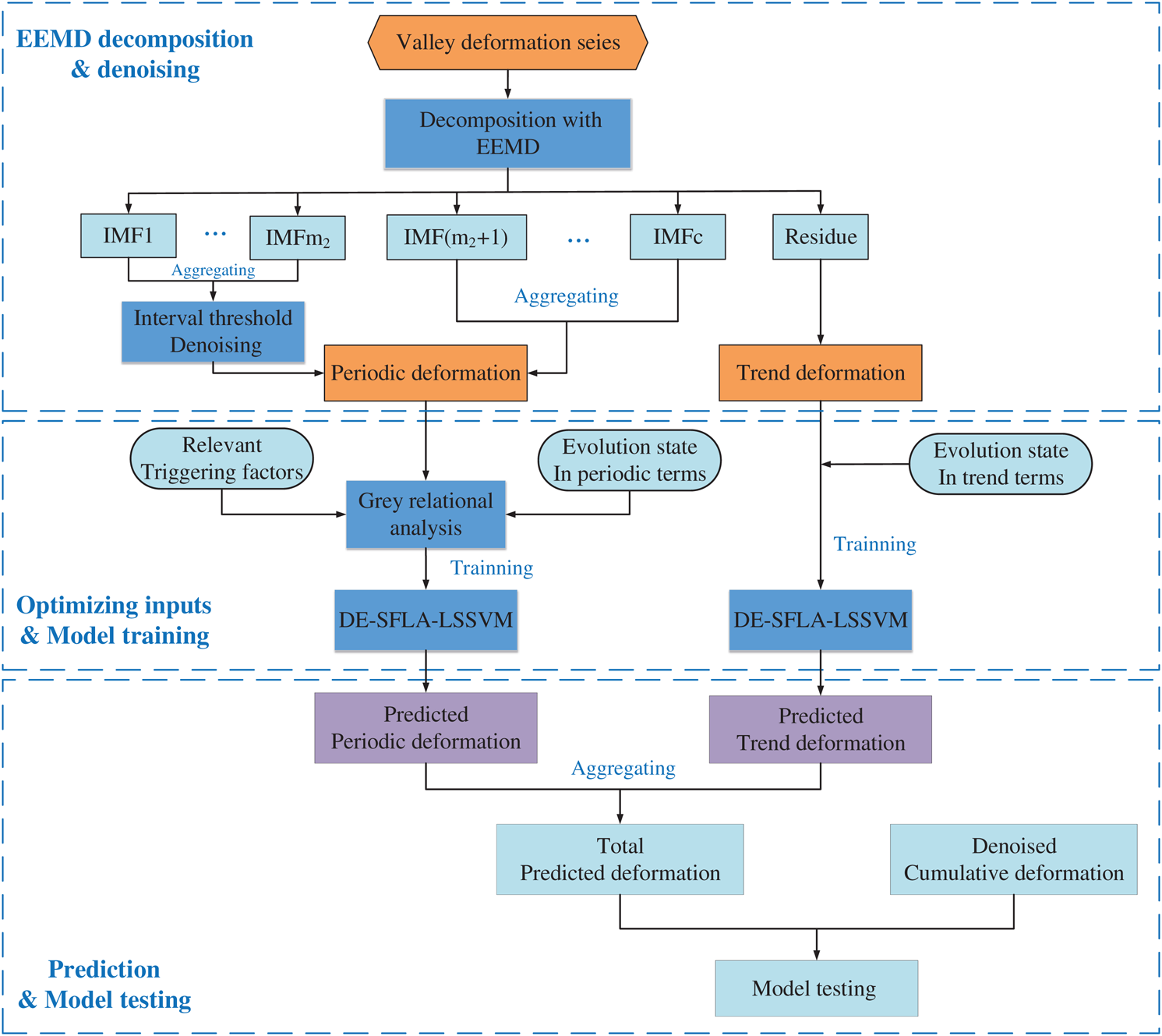
Figure 1: Flowchart of VD prediction with the proposed hybrid model
Step 1 Decomposition and denoising. The original VD series is decomposed into several stationary IMFs and a residue by EEMD, the noise is eliminated from special IMFs. Then, the residue is considered as the trend component, and the remaining IMFs are reconstituted as the periodic deformation.
Step 2 Determination of the input variables. For the periodic deformation, the GRA method [38] is applied to derive the optimal inputs with the relation degree index. For the trend deformation, the previous evolution state is used as the input features.
Step 3 Model training. The input series can be divided into a training set and a testing set. Through learning the training set, the  and
and  in the LSSVM model are optimized with DE-SFLA for a good regression performance. Considering the different mechanisms of the trend and period deformation, DE-SFLA-LSSVM is separately trained for each term to capture the nonlinear patterns.
Step 4 Prediction and ensemble. Using the trained hybrid models to predict the two components with the input features obtained by Step 2, respectively. Then, the final prediction is subsequently obtained by aggregating the two individual forecast results.
Xiluodu hydropower station is located at the Xiluodu canyon of Jinsha river, which is between Yongshan County of the Yunnan Province and Leibo County of the Sichuan Province. The Xiluodu dam is a concrete double curvature arch dam with a maximum height of 285.5 m and a dam crest elevation of 610.0 m. The normal impoundment water level and dead water level of Xiluodu reservoir are 600.0 m and 540.0 m, respectively. As presented in Fig. 2, a total of nine valley survey lines (VD01-VD09) with the elevation between 561.0 m and 749.0 m are configured to monitor the cumulative VD using laser ranging technology. Moreover, there is a meteorological station of Leibo County, which is approximately 7.5 km away from the dam site, recording the daily precipitation and atmospheric temperature. Based on the monitoring system, an approximately six-year record of accumulated VD series, reservoir level, and meteorological data are available since December 2012.
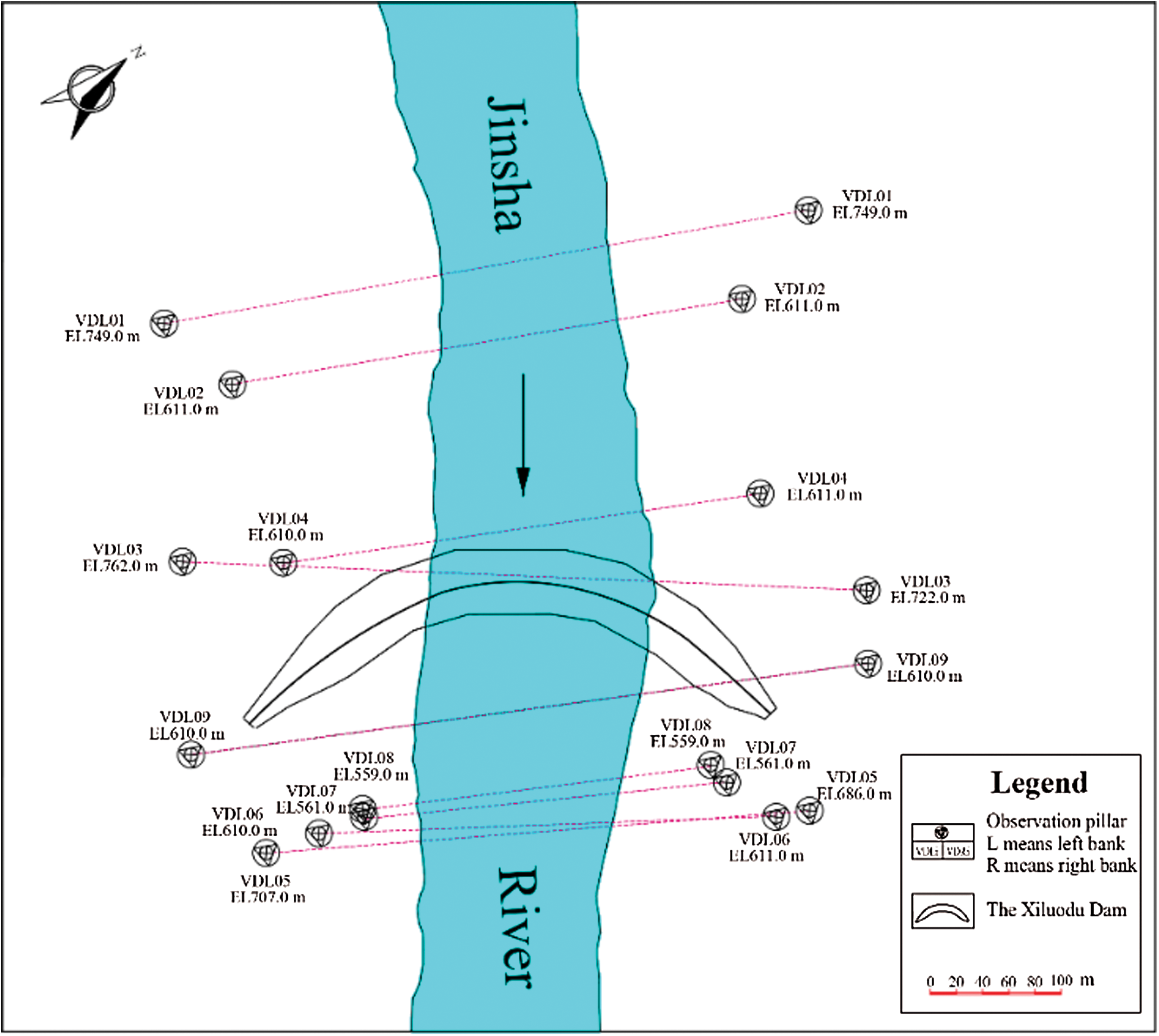
Figure 2: Layout of the survey lines in the dam area
For simplicity and better understanding, the reservoir storage depth (RSD) is defined as the elevation difference between the reservoir level and the riverbed foundation (at an elevation of 324.50 m) to represent the reservoir level fluctuation. According to the field monitoring, the survey line VD03 at the upstream contracted a maximal deformation of 89.54 mm, besides the arch dam structure is particularly sensitive to shrinkage deformation at the abutment. Moreover, the survey line VD05, which is installed downstream and located far away from the dam, can be less affected by the hydraulic structures. Therefore, in this study, the recorded VD time series of VD03 and VD05, RSD, precipitation, and atmospheric temperature from December 2012 to October 2018 are selected for model training and testing. Fig. 3 shows the correlation curves among the cumulative narrowing deformation, RSD, and meteorological data. The climate of the research region exhibits a typical valley and alpine meteorological characteristics with an annual average temperature of 19.7°C, and annual precipitation between 547.3 mm and 833.0 mm. The reservoir began to impound in December 2012 and first reached the maximum reservoir level in October 2014. Since then, the RSD fluctuated between 220.5 m and 275.5 m during the operation regulation of a hydrological year (from June to May in the following year).
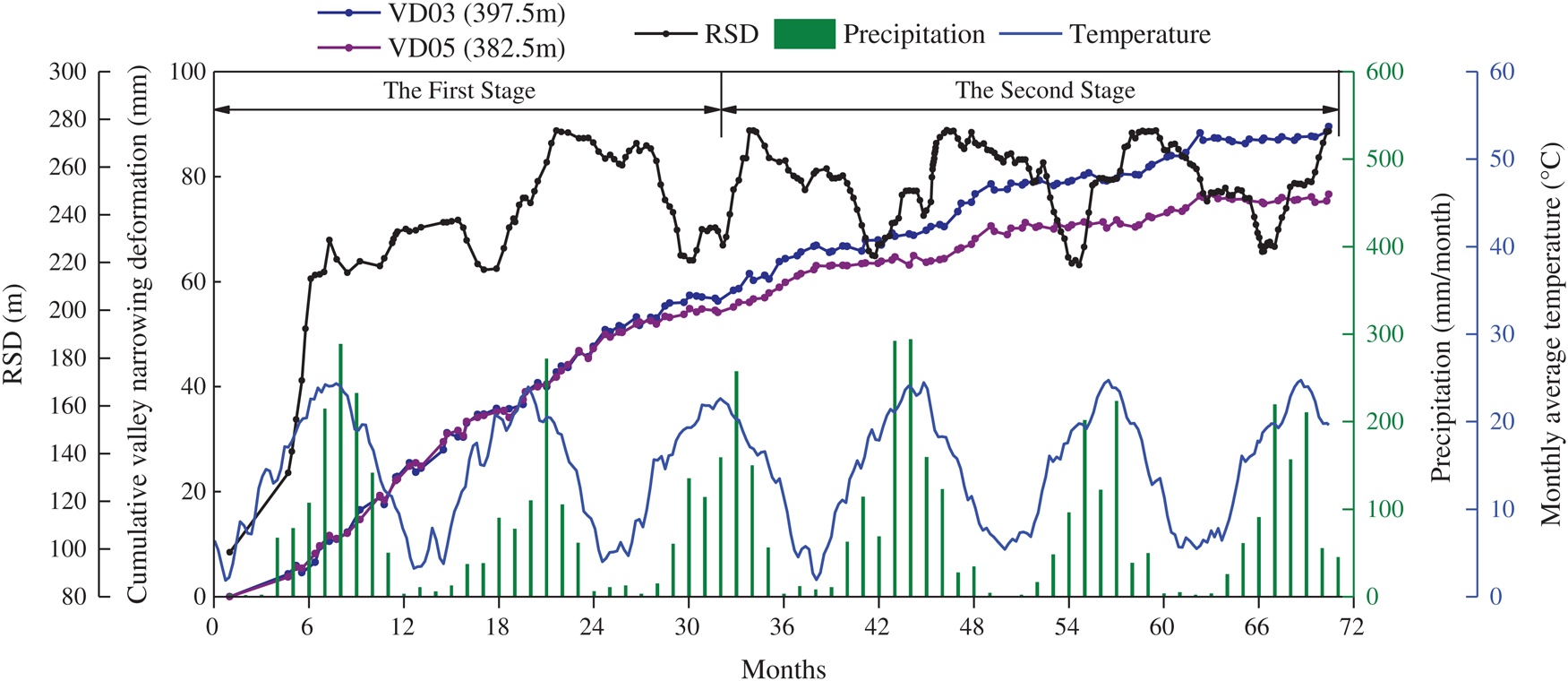
Figure 3: The correlation curves among the precipitation, temperature, RSD, and cumulative VD of VD03 and VD05
As shown in Fig. 3, the evolution of VD exhibits the same tendency, but at different rates. The total deformation of VD03 and VD05 is 89.54 mm and 76.62 mm, respectively. Two distinct phases can be identified, with the demarcation point being the 32nd month for VD03 and VD05. In the first stage (from the 1st month to the 31st month), the valley width has persistently narrowed with an average rate of 1.53–1.94 mm/month, and the maximum rate of 11.44 mm/month. In the second stage (from the 33rd month to the 71st month), an obvious step-like evolution occurred in the curves of cumulative deformation with an average rate of 0.51–0.86 mm/month. Three major “jumps” are observed in the deformation curves around the 35th, 46th, and 58th months, which is characterized by accelerated deformation over a relatively short period followed by a low rate over a long period. Sharp increases of deformation follow the variation of RSD, especially the reservoir impoundment, and the heavy precipitation in the rainy season from June to September every year, which indicates that the combined effect of the RSD fluctuation and precipitation has significant impacts on the VD characters.
4.1 Raw Data Series Decomposition and Denoising Using EEMD-ITD
Since a lack of measured deformation values from December 2012 to May 2013, the dataset from May 2013 to October 2018 was used in this study. EEMD was first performed in MATLAB to decompose the original deformation series of VD03 and VD05 into several IMFs and a residue, respectively. In EEMD, an ensemble member of 100 was used, and the added Gaussian white noise in each ensemble member had a standard deviation of 0.2. Fig. 4 shows the decomposed components from the highest frequency to the residue of the original series. Each VD series was decomposed into five IMFs and one residue, respectively. It can be seen that the residue term is smooth and increases monotonously. The high-frequency IMFs are relatively random fluctuating, while the lower-frequency IMFs are showing periodic fluctuation character.
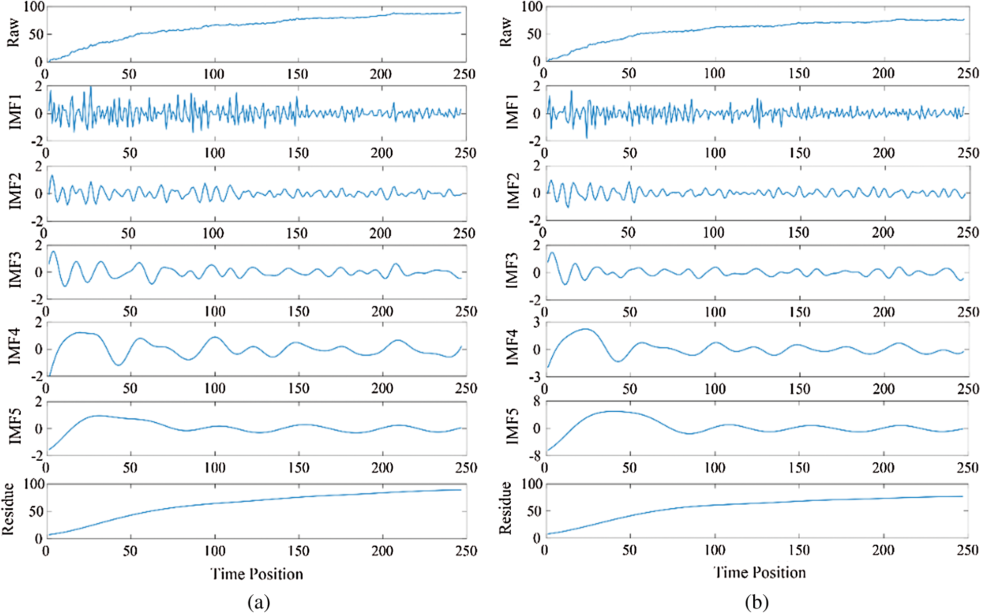
Figure 4: The decomposed IMFs and one residue for two raw time series (a) VD03. (b) VD05
According to the ITD procedure,  and
and  of the two series were determined as 1 and 2 according to [39], respectively, and the thresholds were calculated. After that, the selected IMFs were handled with ITD. The thresholds were 0.742, 0.523 for VD03, and 0.668, 0.471 for VD05, respectively. After the denoising process, two evaluation criteria MSE and SNR are 0.486, 86.821 for VD03, and 0.320, 86.048 for VD05, respectively. In order to evaluate the effectiveness of EEMD-ITD, Discrete wavelet transform (DWT) with the function of Daubechies 4 and the soft threshold method were performed with the wavelet toolbox of MATLAB. After denoised with DWT, two evaluation criteria MSE and SNR are 0.773, 83.340 for VD03, and 0.515, 82.831 for VD05, respectively. It can be qualitatively concluded that: better denoising performance can be achieved by EEMD-ITD compared with DWT, where the MSE is decreased by 37.13% for VD03 and 37.86% for VD05, respectively, and the SNR are increased by 4.01% for VD03 and 3.74% for VD05, respectively.
4.2 Forecast Results of Trend Deformation and Periodic Deformation
The denoised deformation series and the recorded external triggering factors datasets (precipitation, temperature, and RSD) of 65-month were used for the prediction model establishing and validating. The first 55-month dataset was adopted for model training, while the remaining 10-month dataset was employed for model validation. The two denoised IMFs and the remaining three IMFs were reconstituted as the periodic deformation component, and the residue is considered as the trend deformation. Therefore, DE-SFLA-LSSVM models are separately applied to predict the two components with different optimal inputs. It is noted that the validation data is not considered in establishing the forecasting model, and thus the performance of the validation period can represent the real application effect. Therefore, we pay more attention to the forecast performance of the validation period, and just the forecast results of the validation period are shown in the following sections.
4.2.1 Forecast Results of Trend Deformation Component
As shown in Fig. 4, the residue component, which represents the VD evolutionary trend, is a smooth curve with large-scale fluctuations. Since the mechanism of long-term deformation is characterized by the creep behavior of rock masses, which is affected by the internal geological conditions [40]. The DE-SFLA-LSSVM model is applied to predict the trend component. The trend deformation over the past 30 days, 60 days, and 90 days were considered as the input features, while current trend deformation was used as the output. Figs. 5a,5b presents the prediction result of VD03 and VD05 in the validation period, respectively. According to Fig. 5, the DE-SFLA-LSSVM model can well predict the trend component with high forecasting accuracy.
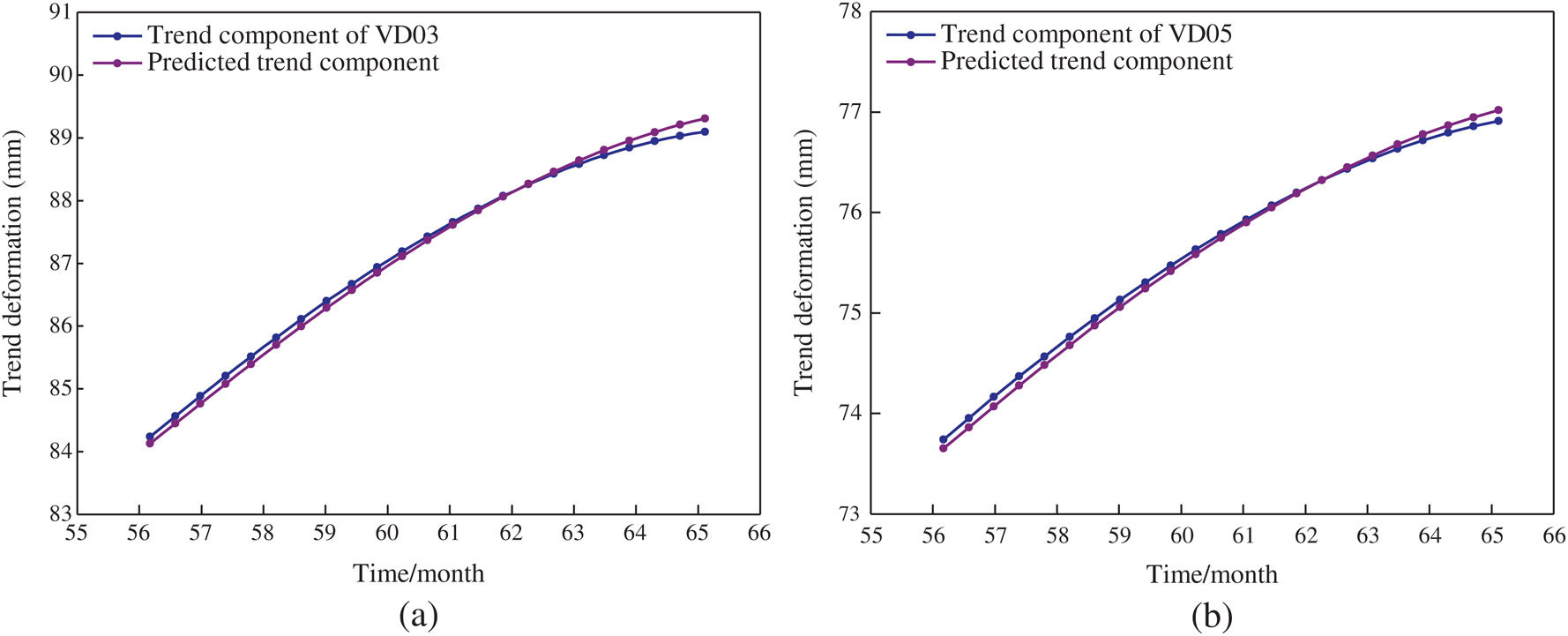
Figure 5: Comparison of the predicted and measured values of the trend component (a) VD03. (b) VD05
Three indicators to evaluate model accuracy and prediction ability in this study consist of the root mean square error (RMSE), mean absolute percentage error (MAPE), and correlation coefficient (R). These indicators are defined as follows:


For VD03, the value of RMSE, MAPE and R is 0.104, 0.106, and 0.999, respectively. The optimal parameters γ and σ2 in LSSVM are 993.493 and 21.508, respectively. For VD05, the value of RMSE, MAPE and R in the validation period is 0.065, 0.076 and 0.999, respectively. The optimal parameters γ and σ2 searched by DE-SFLA are 959.066 and 17.653, respectively.
4.2.2 Forecast Results of Period Deformation Component
Triggering factors analysis and optimal features selection
In order to effectively reconstruct the evolution characters of VD, the mechanics and triggering factors can be considered carefully. According to the analysis of the relationship between the deformation and the external influencing factors in Section 3.2, a total of 13 initial triggering factors were considered [17,41], they are presented as follows:
1.The fluctuation of RSD: in consideration of the lag period of the seepage field adjustment corresponding to reservoir operation, the current RSD (J1) and the average fluctuation rate of RSD over the past 15 days (J2), 30 days (J3), and 60 days (J4) were adopted as the RSD factors.
2.Precipitation: the cumulative antecedent precipitation during the last 15 days (J5), 30 days (J6), and 60 days (J7) were selected as the precipitation factors due to the slow process of precipitation infiltration.
3.Water temperature: the atmospheric temperature in the reservoir region was used to represent the effect of water temperature due to a lack of monitored temperature of river bedrock. The average atmospheric temperature of anterior 15 days (J8), 30 days (J9), and 60 days (J10) were used as the temperature factors.
4.Evolution state: the deformation over the past 15 days (J11), 30 days (J12), and 60 days (J13) are considered.
GRA was employed to quantized the relation degree between the periodic deformation and triggering factors. Datasets of factors were used as the input for GRA, and the optimal inputs were selected from potential factors. The results of GRA are listed in Tab. 1.
Table 1: GRA results of each triggering factor for VD03 and VD05
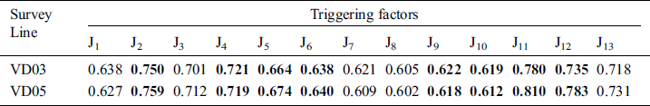
The result indicates that the periodic deformation is significantly influenced by the rate of fluctuation of RSD (J2, J3, and J4), whereas the current RSD (J1) and water temperature factors (J8, J9, and J10) have relatively less influence. As a result, the eight optimal triggering factors were selected as the input features of prediction models, which are highlighted in Tab. 1.
Model parameter settings
The optimal inputs and periodic deformation series were used as the input and output variables, respectively. Datasets were divided into a training set and validation set as same as the modeling of trend componence. To stabilize the learning process of ML models, all input data were normalized in the interval [0,1] using the Minmax normalization.
All these models were developed in MATLAB environment. For the DE-SFLA-LSSVM model, DE-SFLA was applied to optimize the hyper-parameters (γ, σ2) by minimizing the MSE generated in the validation set, the value range of γ and σ2 were set to [0.1,1000]. The initial parameters of DE-SFLA were set as a frog population of 200 (i.e., the size of memeplexes being 20, while each memeplex containing ten frogs), the maximum number of iterations is 100. To study the comparison on the forecasting performance basis of the proposed model, four models including LSSVM, ABC-LSSVM, BPNN, and DE-SFLA-BPNN were performed with the same input features and output vector.
For LSSVM, RBF was chosen as the kernel function, and the hyper-parameters were determined using the grid-search with 5k cross-validation. For ABC-LSSVM, the colony size was 100, the maximum evaluation number was set to 200, the range of γ and σ2 in RBF were set in [0.1,1000]. Moreover, a three-layer BPNN was performed, the nodes of the hidden layer were set to 10, the number of input nodes equaled to the number of optimal features, and the number of output nodes was set to 1.
Forecasting performance
The forecast results of the periodic deformation in the validation period for VD03 and VD05 are shown in Fig. 6. The prediction performance comparison between the proposed model and other LSSVM-based models (i.e., LSSVM and ABC-LSSVM) of VD03 and VD05 is illustrated in Fig. 6a and 6c, respectively. The comparison between the proposed method and ANN-based models (i.e., BPNN and DE-SFLA-BPNN) of VD03 and VD05 is shown in Fig. 6b and 6d, respectively. According to Fig. 6, it demonstrates that the all the predictions show a good agreement with the actual deformation curve on the whole.
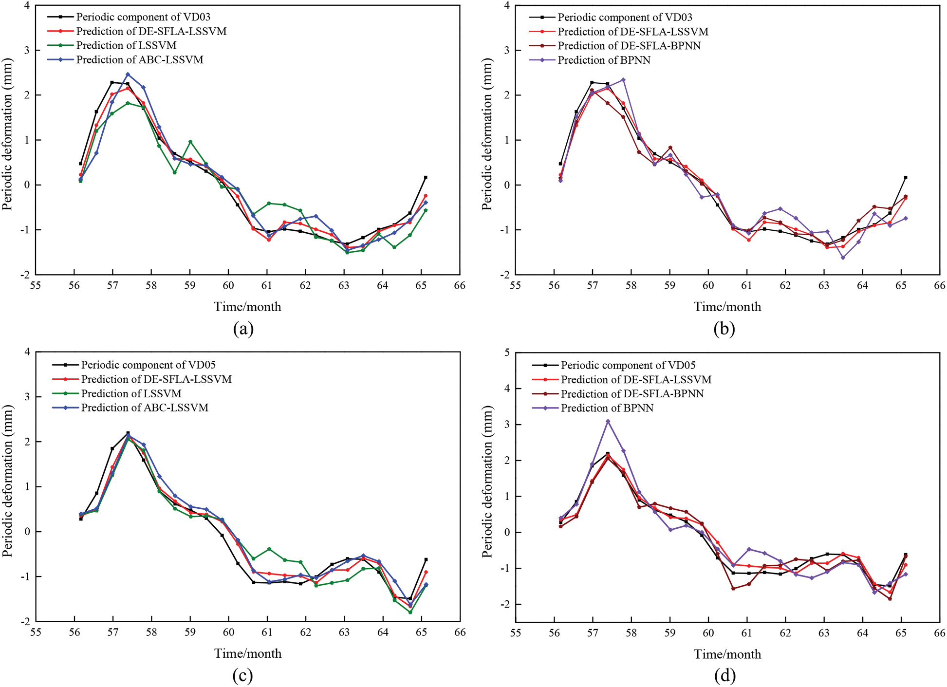
Figure 6: Comparison of the predicted and measured values of the periodic component. (a) prediction of the LSSVM-based models for VD03. (b) prediction of the ANN-based models for VD03. (c) prediction of the LSSVM based models for VD05. (d) prediction of the ANN-based models for VD05
Tab. 2 summarizes forecast results and optimal parameters of the five investigative models. It appears that the proposed model produces higher R values but smaller RMSE and MAPE values in the validation period, whereas LSSVM and BPNN performed worst. More precisely, for VD03, the RMSE, MAPE and R values of DE-SFLA-LSSVM are 0.198, 0.230 and 0.986, respectively, while the accuracy indicators for VD05 are 0.222, 0.297 and 0.978, respectively. Furthermore, the RMSE, MAPE and R of DE-SFLA-BPNN are 0.223, 0.258 and 0.988 for VD03, respectively, While the indicators for VD05 are 0.294, 0.406 and 0.964, respectively. Considering of the three evaluation indices, the performance of DE-SFLA-LSSVM is slightly superior to that of DE-SFLA-BPNN, which suggests that the BPNN model optimized with DE-SFLA has a quite competitive forecasting ability. Taking the period deformation of VD03 for example, the model predictability of DE-SFLA-LSSVM compared with other contrast models.
Table 2: Prediction performance of periodic deformation and optimal parameters
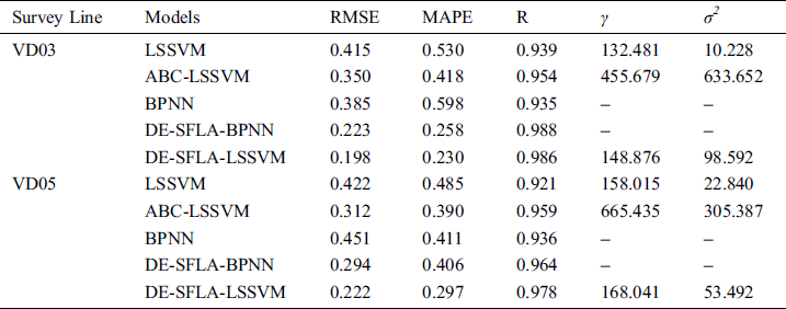
1.Performance comparison between the original models (i.e., LSSVM and BPNN) and hybrid models (i.e., DE-SFLA-LSSVM, ABC-LSSVM, and DE-SFLA-BPNN). It is depicted further from Fig. 6 and Tab. 2, the R value of hybrid models ranges in [0.954,0.988], while the corresponding values of original models ranges in [0.935,0.939]. In addition, the RMSE and MAPE of hybrid models are smaller than that of the two original models. Therefore, the forecasting effect of hybrid models possesses significant promotion with the global searching ability of DE-SFLA and ABC algorithms compared with the two original models. As shown in Fig. 6, it is clear that LSSVM and BPNN cannot well simulate the turning points (e.g., the values of the 57th and 61th month), while the hybrid models are able to maintain the shape of the original periodic deformation well, which greatly helps to improve the prediction accuracy and decrease the forecasting errors. In other words, it can be asserted that hybrid models possess better capabilities to adequately excavate potential information within raw data based on the hyper-parameter optimization of DE-SFLA and ABC algorithms.
2.Performance comparison between DE-SFLA-LSSVM and the LSSVM based models (i.e., LSSVM and ABC-LSSVM). As illustrated in Fig. 6a and Tab. 2, the DE-SFLA-LSSVM models produce better performance in all the LSSVM based models, whereas the ABC-LSSVM model performs well only after the early warning period (the period deformation fluctuates fiercely from the 56th to 59th month). It is clear that ABC-LSSVM shows a poor performance on the amplitudes and appearance time simulating, whereas DE-SFLA-LSSVM has a better agreement with the observed values. In addition, the RMSE and MAPE of ABC-LSSVM are smaller than that of LSSVM, which indicates that the optimization process of DE-SFLA and ABC algorithm has an enhancing effect to the improperly searched ability of grid search method and can well solve the local optimization and over-fitting problems, while DE-SFLA has a stronger global searching and generalization abilities than ABC algorithm.
3.Performance comparison between DE-SFLA-LSSVM and the ANN based models (i.e., BPNN and DE-SFLA-BPNN). Fig. 6b and Tab. 2 displays the comparison forecasting results and performance indexes. Among these models, the fitting performance of DE-SFLA-LSSVM is slightly superior to that of DE-SFLA-BPNN. Moreover, the RMSE and MAPE of DE-SFLA-BPNN are 0.223 and 0.258, while the values of BPNN are 0.385 and 0.598, respectively. The R value of the former model is 0.988, which is greater than that of BPNN (i.e., 0.935). As shown in Fig. 6b, since BPNN starts with a random generation of internal weights and adjusts the network weights and deviations with the back-propagation algorithm, the result of BPNN always tends to fluctuate around actual values, whereas DE-SFLA-BPNN can produce a relatively stable and accurate deformation prediction. It also indicates that the DE-SFLA as an optimization algorithm of LSSVM and BPNN can significantly improve prediction accuracy and generalization abilities.
For VD05, according to the forecast result shown in Fig. 6c and 6d and Tab. 2, the proposed model produced the lowest RMSE and MAPE of 0.222 and 0.297, whereas BPNN has the highest RMSE and MAPE of 0.451 and 0.411, respectively. Moreover, the prediction accuracy of ABC-LSSVM is greater than LSSVM, while DE-SFLA-BPNN performs better than ABC-LSSVM, which indicates that the optimization process of DE-SFLA has an enhancing effect on forecasting performance. Therefore, the performance of the proposed model is further verified.
4.3 Forecast Results of Total Deformation
Finally, the forecast results of the cumulative VD were calculated by reconstructing the predicted trend and periodic deformation results. The comparison between the predicted values and the denoised cumulative deformation in the validation period is shown in Fig. 7 and Tab. 3. It indicates that the forecast results show good agreement with the measured series, and the prediction errors are within an acceptable precision range. Furthermore, the proposed DE-SFLA-LSSVM outperforms other models with better forecast accuracy for VD03 and VD05.
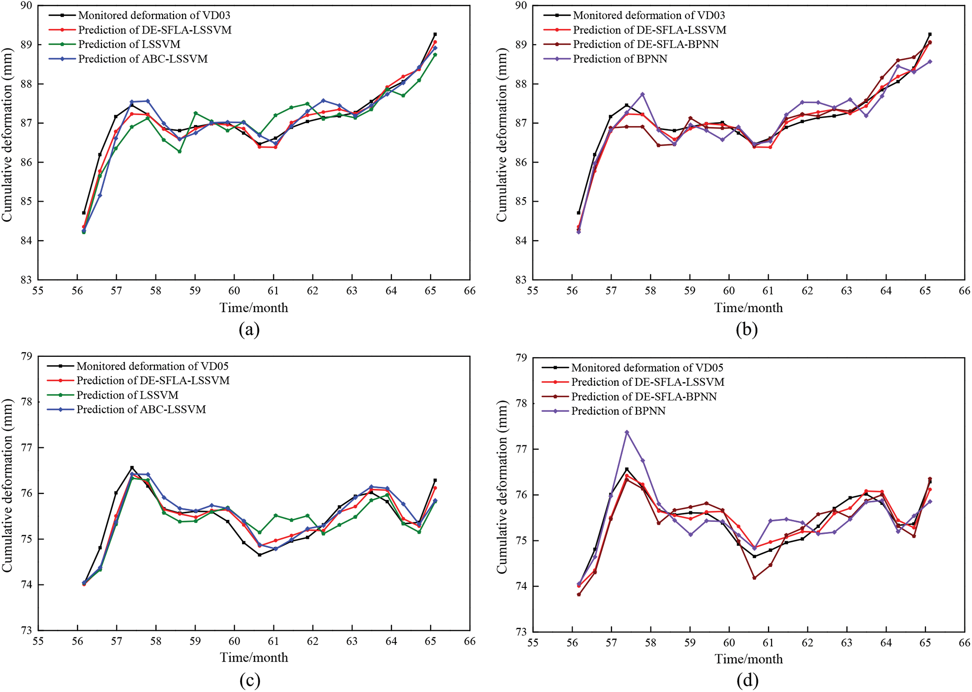
Figure 7: Comparison of the predicted and monitored cumulative deformation in the validation period. (a) prediction of the LSSVM-based models for VD03. (b) prediction of the ANN-based models for VD03. (c) prediction of the LSSVM based models for VD05. (d) prediction of the ANN-based models for VD05
Table 3: Prediction performance of different models for the cumulative deformation
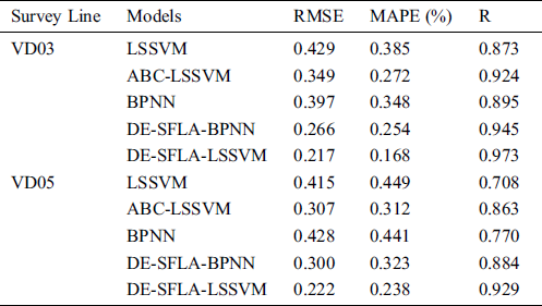
As can be clearly seen in Figs. 7a and 7b and Tab. 3. For VD03, DE-SFLA-LSSVM achieved a higher accuracy with RMSE and MAPE are 0.217 and 0.168, respectively, which are lower than that of other hybrid models (i.e., ABC-LSSVM and DE-SFLA-BPNN). Whereas LSSVM is the worst-performing model with the RMSE, MAPE, and R being 0.429, 0.385 and 0.873, respectively. The original LSSVM and BPNN model provides unsatisfactory performance in the total deformation prediction due to the accumulation prediction errors of the periodic deformation. When hybrid models are taken into consideration, the proposed DE-SFLA-LSSVM, ABC-LSSVM and DE-SFLA-BPNN models outperform LSSVM and BPNN all the time. It indicates that DE-SFLA and ABC are efficient algorithms for optimizing the parameters in the LSSVM and BPNN models.
As illustrated in Figs. 7c and 7d and Tab. 3. For VD05, the RMSE, MAPE, and R of DE-SFLA-LSSVM are 0.222, 0.238 and 0.929, respectively, which indicates that DE-SFLA-LSSVM method exhibits a better performance in terms of accuracy and percentage error than those compact models. BPNN is the worst-performing model with the RMSE, MAPE, and R being 0.428, 0.441 and 0.770, respectively. Note that the higher R indicates that the proposed model results in a better agreement with the actual values, and the lower RMSE and RMSE demonstrate lower average prediction errors.
By comparison, it is indicated that using the proposed DE-SFLA-LSSVM model for trend and periodic deformation prediction by considering the relevant triggering factors can provide better predictive performance for cumulative VD prediction. Generally, the prediction performance of the DE-SFLA-LSSVM model outperforms that of all the BPNN-based models and LSSVM-based models. The deformation series cannot be perfectly predicted by LSSVM and BPNN due to the improperly searched ability of the grid search method and the random generated internal weights and the simple structure of BPNN. Nevertheless, the DE-SFLA-LSSVM model and DE-SFLA-BPNN model exhibit better performance in terms of accuracy and percentage error in the validation period for VD prediction.
This paper studies the VD prediction by using a novel hybrid forecasting model that is made up of EEMD-ITD and DE-SFLA-LSSVM. The performance of LSSVM has much to do with the preprocessing of non-stationary and noisy series and optimizing the hyper-parameters. Two actual VD series monitored in Xiluodu reservoir region are used for model testing, and the forecast performance of the proposed model is validated and outperforms other common methods.
According to the corresponding comprehensive analysis, the EEMD-ITD denoising procedure can adequately maintain the major evolution features of the original series, while the redundant noise is eliminated. By comparing with WTD, EEMD-ITD achieved better performance with higher SNR and lower MSE of 0.486, 86.821 for VD03, and 0.320, 86.048 forVD05, respectively. It reveals that the introduced EEMD-ITD is an effective denoising method for signal preprocessing. The result of GRA indicates that the periodic deformation is significantly influenced by the rate of fluctuation of RSD, whereas the current RSD and temperature have less influence on VD. Moreover, GRA removes redundant information and extracts the relevant factors, which can reduce the model complexity and improves prediction performance. The performance of DE-SFLA-LSSVM and other conventional methods including LSSVM, ABC-LSSVM, BPNN, and DE-SFLA-BPNN is validated and compared for the periodic deformation forecasting. The result shows that the proposed hybrid model outperforms the other methods with high precision. Therefore, the proposed hybrid model has the potential to be applied for the early-warning in Xiluodu project.
Acknowledgement: Special thanks are given to the journal editors and anonymous reviewers for their valuable comments and suggested revisions.
Funding Statement: This research is supported by the National Key R&D Program of China (No. 2018YFC0407004), and the National Natural Science Foundation Project of China (No. 11772118).
Conflicts of Interest: The authors declare that they have no conflicts of interest to report regarding the present study.
1. L. Cheng, Y. Liu, Q. Yang, Y. Pan and Z. Lv. (2017). “Mechanism and numerical simulation of reservoir slope deformation during impounding of high arch dams based on nonlinear FEM,” Computers and Geotechnics, vol. 81, pp. 143–154.
2. Y. Liu, X. Wang, Z. Wu, Z. He and Q. Yang. (2018). “Simulation of landslide-induced surges and analysis of impact on dam based on stability evaluation of reservoir bank slope,” Landslides, vol. 15, no. 10, pp. 2031–2045.
3. C. Zangerl, K. Evans, E. Eberhardt and S. Loew. (2008). “Consolidation settlements above deep tunnels in fractured crystalline rock: Part 1—Investigations above the Gotthard highway tunnel,” International Journal of Rock Mechanics and Mining Sciences, vol. 45, no. 8, pp. 1195–1210.
4. J. Yang, D. Hu and W. Guan. (2005). “Analysis of high slope rock deformation and safety performance for left bank of Lijiaxia arch dam,” Chinese Journal of Rock Mechanics and Engineering, vol. 24, no. 19, pp. 3551–3560.
5. J. Zhang, W. Xu, H. Jin, D. Liu and D. Cai. (2009). “Safety monitoring and stability analysis of large-scale and complicated high rock slope,” Chinese Journal of Rock Mechanics and Engineering, vol. 28, no. 9, pp. 1819–1827.
6. Q. J. Zhou, G. X. Zhang and Y. Liu. (2013). “Prediction of and early warning for deformation and stress in the Xiaowan arch dam during the first impounding stage,” Applied Mechanics and Materials, vol. 405-408, pp. 2463–2472.
7. G. Liang, Y. Hu, Q. Fan and Q. Li. (2016). “Analysis on valley deformation of Xiluodu high arch dam during impoundment and its influencing factors,” Journal of Hydroelectric Engineering, vol. 35, no. 9, pp. 101–110.
8. Q. Yang, Y. Pan, L. Cheng, Y. Liu, Z. Zhou et al. (2015). , “Mechanism of valley deformation of high arch dam and effective stress principle for unsaturated fractured rock mass,” Chinese Journal of Rock Mechanics and Engineering, vol. 34, no. 11, pp. 2258–2269.
9. G. G. Anagnostopoulos, S. Fatichi and P. Burlando. (2015). “An advanced process-based distributed model for the investigation of rainfall-induced landslides: The effect of process representation and boundary conditions,” Water Resources Research, vol. 51, no. 9, pp. 7501–7523.
10. D. Song, A. Che, R. Zhu and X. Ge. (2018). “Dynamic response characteristics of a rock slope with discontinuous joints under the combined action of earthquakes and rapid water drawdown,” Landslides, vol. 15, no. 6, pp. 1109–1125.
11. L. Yan, W. Xu, H. Wang, R. Wang, Q. Meng et al. (2019). , “Drainage controls on the Donglingxing landslide (China) induced by rainfall and fluctuation in reservoir water levels,” Landslides, vol. 16, no. 8, pp. 1583–1593.
12. Q. Hou, G. Wu, H. Li, G. Fan and J. Zhou. (2019). “Large deformation and failure mechanism analyses of Tangba high slope with a high-intensity and complex excavation process,” Journal of Mountain Science, vol. 16, no. 2, pp. 453–469.
13. P. Lin, X. Liu, S. Hu and P. Li. (2016). “Large deformation analysis of a high steep slope relating to the Laxiwa reservoir, China,” Rock Mechanics and Rock Engineering, vol. 49, no. 6, pp. 2253–2276.
14. T. Yin, Q. Li, Y. Hu, S. Yu and G. Liang. (2020). “Coupled thermo-hydro–mechanical analysis of valley narrowing deformation of high arch dam: A case study of the Xiluodu project in China,” Applied Sciences, vol. 10, no. 2, pp. 524.
15. M. Li, Z. Zhou, C. Zhuang, Y. Xin, M.Chen et al. (2020). , “The cause and statistical analysis of the river valley contractions at the Xiluodu hydropower station, China,” Water, vol. 12, no. 3, pp. 791.
16. G. Liang, Y. Hu and Q. Li. (2018). “Safety monitoring of high arch dams in initial operation period using vector error correction model,” Rock Mechanics and Rock Engineering, vol. 51, no. 8, pp. 2469–2481.
17. Z. Guo, L. Chen, L. Gui, J. Du, K.Yin et al. (2019). , “Landslide displacement prediction based on variational mode decomposition and WA-GWO–BP model,” Landslides, vol. 17, pp. 1–17.
18. S. Xu and R. Niu. (2018). “Displacement prediction of Baijiabao landslide based on empirical mode decomposition and long short-term memory neural network in Three Gorges area, China,” Computers & Geosciences, vol. 111, pp. 87–96.
19. X. Zhu, Q. Xu, M. Tang, W. Nie, S. Ma et al. (2017). , “Comparison of two optimized machine learning models for predicting displacement of rainfall-induced landslide: A case study in Sichuan Province, China,” Engineering Geology, vol. 218, pp. 213–222.
20. Z. Cai, W. Xu, Y. Meng, C. Shi and R. Wang. (2016). “Prediction of landslide displacement based on GA-LSSVM with multiple factors,” Bulletin of Engineering Geology and the Environment, vol. 75, no. 2, pp. 637–646.
21. H. Li, Q. Xu, Y. He and J. Deng. (2018). “Prediction of landslide displacement with an ensemble-based extreme learning machine and copula models,” Landslides, vol. 15, no. 10, pp. 2047–2059.
22. N. N. Vasu and S. R. Lee. (2016). “A hybrid feature selection algorithm integrating an extreme learning machine for landslide susceptibility modeling of Mt. Woomyeon, South Korea,” Geomorphology, vol. 263, pp. 50–70.
23. J. A. Suykens and J. Vandewalle. (1999). “Least squares support vector machine classifiers,” Neural Processing Letters, vol. 9, no. 3, pp. 293–300.
24. T. Wen, H. Tang, Y. Wang, C. Lin and C. Xiong. (2017). “Landslide displacement prediction using the GA-LSSVM model and time series analysis: A case study of Three Gorges reservoir, China,” Natural Hazards and Earth System Sciences, vol. 17, no. 12, pp. 1–20.
25. C. Liu, Z. Jiang, X. Han and W. Zhou. (2019). “Slope displacement prediction using sequential intelligent computing algorithms,” Measurement, vol. 134, pp. 634–648.
26. W. Jia, D. Zhao, Y. Zheng and S. Hou. (2019). “A novel optimized GA−Elman neural network algorithm,” Neural Computing and Applications, vol. 31, no. 2, pp. 449–459.
27. B. Xiang. (2019). “An improved unsupervised image segmentation method based on multi-objective particle swarm optimization clustering algorithm,” Computers, Materials & Continua, vol. 58, no. 2, pp. 451–461.
28. D. Tien Bui, T. A. Tuan, N-D. Hoang, N. Q. Thanh, D. B. Nguyen et al. (2017). , “Spatial prediction of rainfall-induced landslides for the Lao Cai area (Vietnam) using a hybrid intelligent approach of least squares support vector machines inference model and artificial bee colony optimization,” Landslides, vol. 14, no. 2, pp. 447–458.
29. M. Eusuff, K. Lansey and F. Pasha. (2006). “Shuffled frog-leaping algorithm: A memetic meta-heuristic for discrete optimization,” Engineering Optimization, vol. 38, no. 2, pp. 129–154.
30. D. Tang, J. Yang, S. Dong and Z. Liu. (2016). “A lévy flight-based shuffled frog-leaping algorithm and its applications for continuous optimization problems,” Applied Soft Computing, vol. 49, pp. 641–662.
31. G. Fang, Y. Guo, X. Wen, X. Fu, X. Lei et al. (2018). , “Multi-objective differential evolution-chaos shuffled frog leaping algorithm for water resources system optimization,” Water Resources Management, vol. 32, no. 12, pp. 3835–3852.
32. S. Ghimire, R. C. Deo, N. Raj and J. Mi. (2019). “Wavelet-based 3-phase hybrid SVR model trained with satellite-derived predictors, particle swarm optimization and maximum overlap discrete wavelet transform for solar radiation prediction,” Renewable and Sustainable Energy Reviews, vol. 113, pp. 109247.
33. Y. Xiang, L. Gou, L. He, S. Xia and W. Wang. (2018). “A SVR-ANN combined model based on ensemble EMD for rainfall prediction,” Applied Soft Computing, vol. 73, pp. 874–883.
34. T. Wang, M. Zhang, Q. Yu and H. Zhang. (2012). “Comparing the applications of EMD and EEMD on time−frequency analysis of seismic signal,” Journal of Applied Geophysics, vol. 83, pp. 29–34.
35. Z. Wu and N. E. Huang. (2011). “Ensemble empirical mode decomposition: A noise-assisted data analysis method,” Advances in Adaptive Data Analysis, vol. 01, no. 01, pp. 1–41.
36. Y. Kopsinis and S. McLaughlin. (2009). “Development of EMD-based denoising methods inspired by wavelet thresholding,” IEEE Transactions on Signal Processing, vol. 57, no. 4, pp. 1351–1362.
37. G. Rilling and P. Flandrin. (2008). “One or two frequencies? The empirical mode decomposition answers,” IEEE Transactions on Signal Processing, vol. 56, no. 1, pp. 85–95.
38. J. Deng. (1989). “Introduction to grey system theory,” The Journal of Grey System, vol. 1, no. 1, pp. 1–24.
39. G. Yang, Y. Liu, Y. Wang and Z. Zhu. (2015). “EMD interval thresholding denoising based on similarity measure to select relevant modes,” Signal Processing, vol. 109, pp. 95–109.
40. C. Zhou, K. Yin, Y. Cao, E. Intrieri, B. Ahmed et al. (2018). , “Displacement prediction of step-like landslide by applying a novel kernel extreme learning machine method,” Landslides, vol. 15, no. 11, pp. 2211–2225.
41. J. Du, K. Yin and S. Lacasse. (2013). “Displacement prediction in colluvial landslides, Three Gorges Reservoir, China,” Landslides, vol. 10, no. 2, pp. 203–218.
 | This work is licensed under a Creative Commons Attribution 4.0 International License, which permits unrestricted use, distribution, and reproduction in any medium, provided the original work is properly cited. |