DOI:10.32604/cmc.2020.012517
| Computers, Materials & Continua DOI:10.32604/cmc.2020.012517 | |
| Article |
An Adaptive Vision Navigation Algorithm in Agricultural IoT System for Smart Agricultural Robots
1School of Computer science, Inner Mongolia University, Hohhot, 010021, China
2Key Laboratory of Wireless Networks and Mobile Computing, School of Computer Science, Inner Mongolia University, Hohhot, 010021, China
3Simulation Center, Air Force Early Warning Academy, Wuhan, 430019, China
*Corresponding Author: Zhibin Zhang. Email: cszhibin@imu.edu.cn
Received: 02 July 2020; Accepted: 14 September 2020
Abstract: As the agricultural internet of things (IoT) technology has evolved, smart agricultural robots needs to have both flexibility and adaptability when moving in complex field environments. In this paper, we propose the concept of a vision-based navigation system for the agricultural IoT and a binocular vision navigation algorithm for smart agricultural robots, which can fuse the edge contour and the height information of rows of crop in images to extract the navigation parameters. First, the speeded-up robust feature (SURF) extracting and matching algorithm is used to obtain featuring point pairs from the green crop row images observed by the binocular parallel vision system. Then the confidence density image is constructed by integrating the enhanced elevation image and the corresponding binarized crop row image, where the edge contour and the height information of crop row are fused to extract the navigation parameters (θ, d) based on the model of a smart agricultural robot. Finally, the five navigation network instruction sets are designed based on the navigation angle θ and the lateral distance d, which represent the basic movements for a certain type of smart agricultural robot working in a field. Simulated experimental results in the laboratory show that the algorithm proposed in this study is effective with small turning errors and low standard deviations, and can provide a valuable reference for the further practical application of binocular vision navigation systems in smart agricultural robots in the agricultural IoT system.
Keywords: Smart agriculture robot; 3D vision guidance; confidence density image; guidance information extraction; agriculture IoT
There are many vision-based technologies used in applications of autonomous robots [1–3] or other applications such as the real-time visual tracking shape and colour feature of object in the literature [4]. Traditional agricultural robots based on vision technology have obtained great success [5,6], and can be operated in several stages of a process to solve the demanding problems in agricultural production [7]. Many researchers have studied robot navigation [8], mainly focusing on crop-row line detection. However, the field environment is so complex that the navigation information extraction is not only affected by factors such as weeds and variations in illumination, but is also influenced by the irregular growth of crops. The irregularity of crop plant growth is particularly obvious in the late growth stage when the inter-row spaces are narrow, making automatic navigation difficult for traditional agricultural robots guided by vision technology. Thus, it is necessary to develop a smart agricultural robot that can automatically adjust its posture in real-time to adaptively move along an irregular crop row, and can also be maneuvered by the control instruction of the IoT node [9]. This will prevent unevenly growing crop plants from being crushed during the automatic navigation process. Moreover, the smart agricultural robot can also overcome the deficiencies of crop-row line detection due to dynamic and unpredictable situations such as fixed obstacles [10], which create issues for traditional agricultural robots.
The line-detection vision navigation algorithms of traditional agricultural robots have been proposed using different crop-row recognition methods for different field applications [11–13]. Searcy et al. [14] applied the Hough transform to the extraction of navigation parameters of agricultural robots. In [15] the excess green method was used to separate green crops from their soil background, and then vertical projection was used to determine the candidate points of crop centerlines to extract the row line. The authors of [16] proposed a vision approach for row recognition based on the grayscale Hough transform on intelligently merged images, which was able to detect crop rows at the various growth stages. In [17] a novel automatic and robust crop row detection method based on maize field images was proposed. Some navigation algorithms based on stereo vision technology for crop row recognition have also been proposed. For instance, in [18], after a three-dimensional (3D) crop-row structure map of an entire field was created using the acquired images, a feature point tracking algorithm was used to extract a tractor motion indicated by the feature points from continuous stereo images, and then feed the outcomes to a dynamic model of the tractor to estimate its traveling speed and heading direction. In [19], a stereo vision-based 3D egomotion estimation system was proposed to track the features in image sequences, in which those feature points were matched to obtain the 3D point clouds for motion estimation. The authors of [20] proposed an unsupervised algorithm for vineyard detection and evaluation of vine row features based on the processing of 3D point-cloud maps, in which the information on local vine row orientations and local inter-row distances were organized in geo-referenced maps to allow the automatic path planning along the inter-row spaces. In [21] a branch detection method was developed, which used the depth features and a region-based convolutional neural network (R-CNN) for detection and localization of branches.
However, the aforementioned research does not address the edge information of plant leaves when agricultural robots are advancing along a crop row using two-dimensional (2D) or 3D row-line recognition, and the methods did not employ IoT technology [22]. This paper proposes a vision navigation algorithm based on the 3D morphological edge and height information of crop rows to guide a smart agricultural robot to adapt to irregular crop rows to avoid crushing crops. Furthermore, the smart agricultural robot advancing along crop rows can obtain essential real-time non-destructive crop growth information. This information can then be transmitted to a cloud computing server in the smart agriculture IoT system to predict the yield and evaluate the health status of crops. This study makes two primary contributions: 1) We propose the concept of a smart agricultural robot vision navigation system for use in the agricultural IoT; and 2) We propose an adaptive vision navigation algorithm for the smart agricultural robot.
2 Smart Agricultural Robot Navigation IoT System
To enable the automatic navigation of a smart agricultural robot, we designed a smart agricultural robot navigation IoT system according to the literature [23]. As shown in Fig. 1, in this system an image acquisition layer is used to collect information, a transmission layer is used to transmit data, and a cloud computing layer provides complex computing services. After processing the data in the cloud computing layer, the results are transmitted to the controller through the transmission layer.
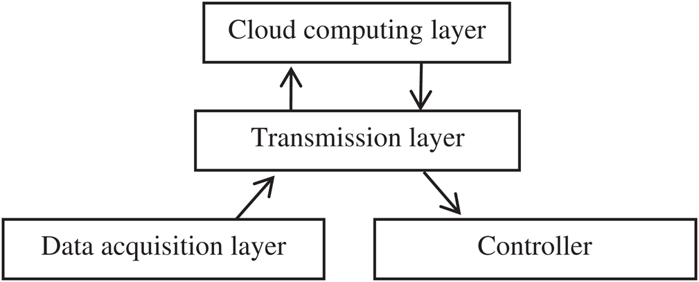
Figure 1: Framework of the agricultural IoT system for the smart agricultural robot
The function modules of the smart agricultural robot are shown in Fig. 2.
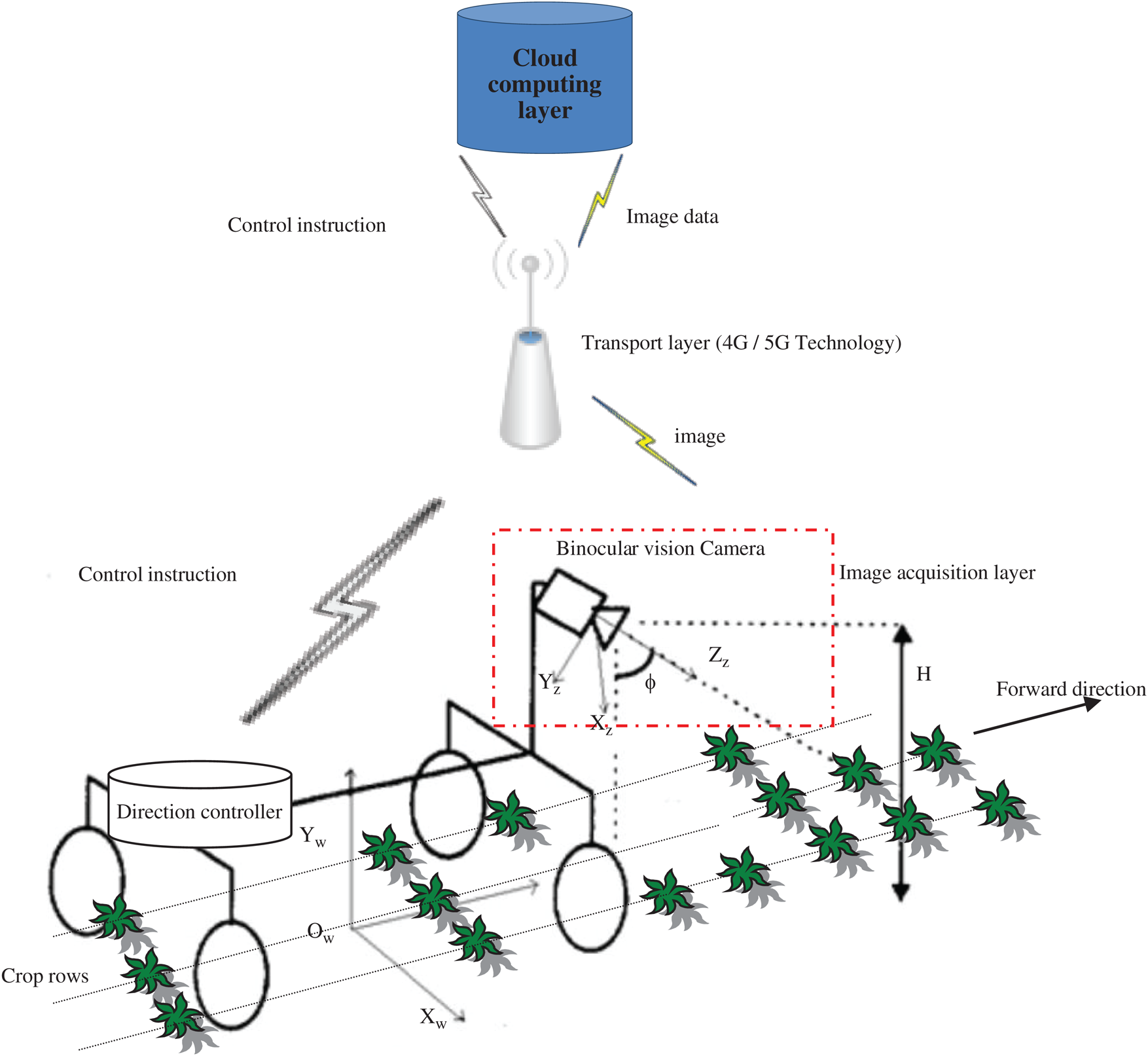
Figure 2: Function modules of the smart agriculture robot embedded in an agricultural IoT system
In the data acquisition layer, the image data are acquired by using a Bumblebee2 binocular stereoscopic camera installed on the agricultural robot to observe green crops in real time. In the transmission layer, the collected image data are transmitted in real time to the cloud computing layer through 4G/5G protocols. In the cloud computing layer, we propose an adaptive vision navigation algorithm for the agricultural robot, which fuses the 2D and 3D information of the green crop feature points to obtain the navigation parameters of the smart agricultural robot. The robot’s control center can also receive the control instructions of the cloud computing services in order to complete autonomous navigation tasks. These IoT capabilities can improve the robustness, flexibility, and reliability of the smart agricultural robot.
3 Adaptive Vision Navigation Implementation
Stereo matching is the process of constructing the corresponding pairs in the left and right images from different perspectives of an object. When these points are matched, their 3D information can be obtained by using Eq. (1), where Zc is the camera coordinate; Xw, Yw, and Zw are the world coordinates; and xr and yr are the image coordinates. The relationships of the coordinates are shown in Fig. 3. We use the right image as the reference image.
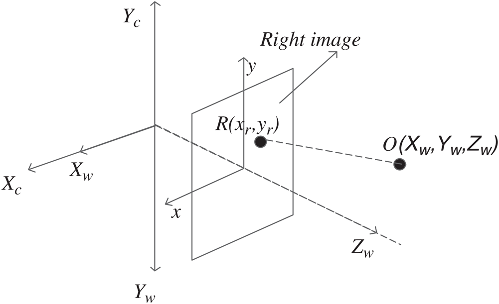
Figure 3: Diagram of relationships between the world coordinate, camera coordinate, and image coordinate systems
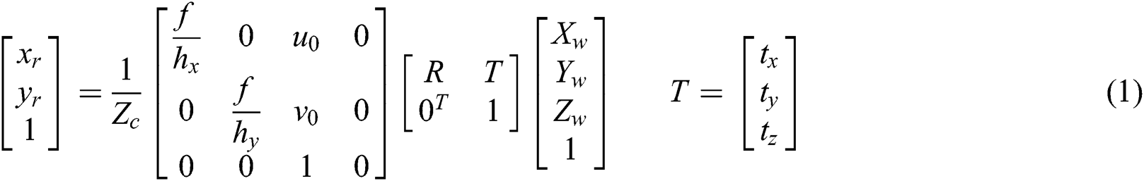
In Eq. (1), the rotation matrix R and the translation vector T contain the pose parameters of a camera relative to the world coordinate system [24], which are called external parameters; hx and hy represent the physical scale of each pixel in the image coordinates, together with the focal length of camera lens f, which are called internal parameters. The origin of the image coordinate is (u0, v0), with 0T = (0, 0, 0). Internal and external parameters can be obtained by the camera calibration process [25]. Based on the parallel binocular vision model, in this study the speeded-up robust feature (SURF) extracting and matching algorithm [26] is used to obtain the 3D spatial information of corresponding pairs of green crop rows. The matched features are shown in Fig. 4. Then, the elevation image of the crop row can be obtained. As shown in Fig. 5a, the brighter the feature point region in the elevation image, the higher its representing crop row height, according to Eq. (2).
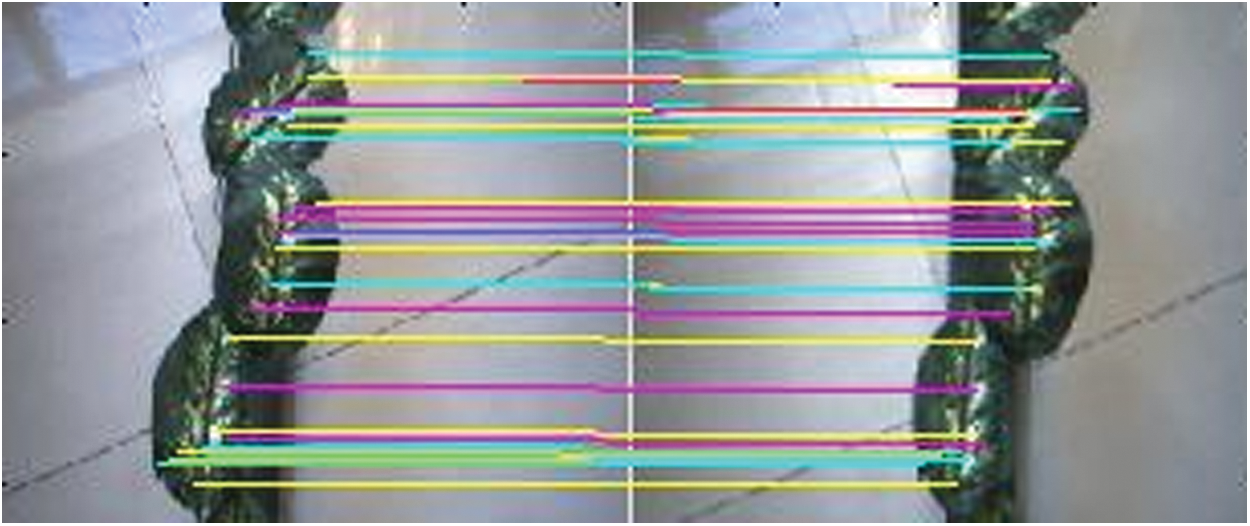
Figure 4: Results of SURF feature extracting and matching
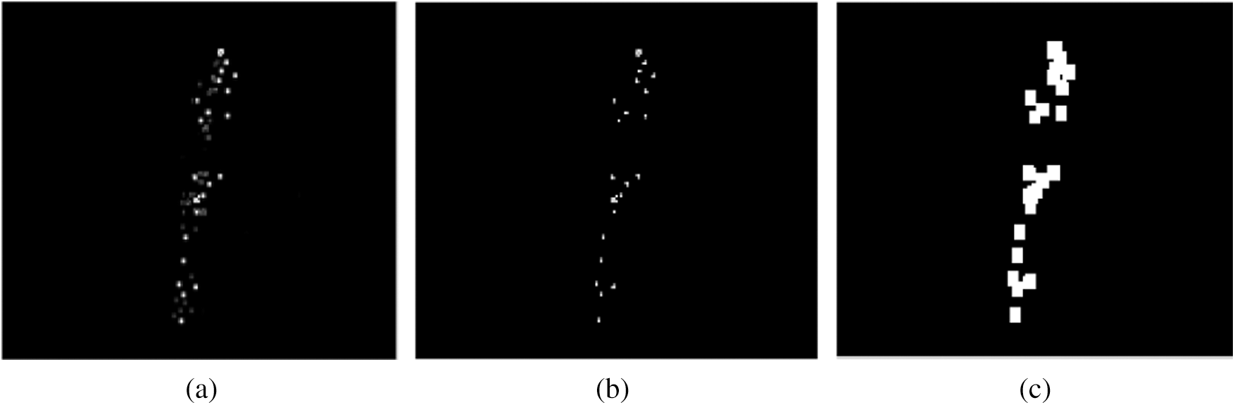
Figure 5: Process of producing enhanced elevation images (a) Elevation image (b) Filtered image (c) Enhanced image

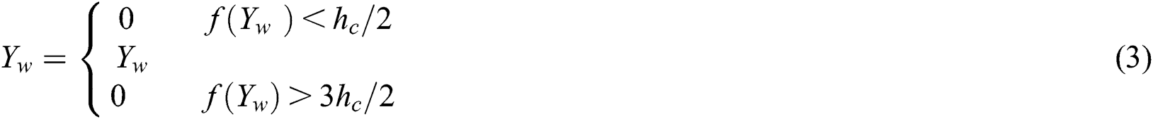
In Eq. (2), the signs max and min denote taking a maximum and minimum from Yw, respectively. The function f(Yw) represents a grayscale value at a certain point about Yw, denoting the height of the crops in the elevation image. Considering the 3D morphological and structural characteristics of the crop rows are roughly consistent relative to weeds or other plants in the field, we aim to preserve certain heights of the crop plants according to Eq. (3) to improve the robustness of detecting crop rows, where hc is a threshold value (hc = 16 in the experiments); Yw ∈ (0, 25) cm, f(Yw) ∈ (0, 255). The processed result is shown in Fig. 5b.
From Fig. 5b, we see that the points that do not meet the height requirement are completely removed. However, the available feature points are relatively sparse, resulting in poor functionality in the elevation image. To eliminate the impact of sparse feature points in elevation images, we dilate the feature points in the adjacent regions by using the morphological dilatation operator with a template size of 4 × 4. A typical resulting image is shown in Fig. 5c. In this way, the regions of feature points will be extended to some extent in the elevation image to increase the stability and reliability of the process of extracting navigation parameters.
The elevation image emphasizes only the height information of the crop row, but the crop row edge information is also important for the navigation system of the agricultural robot, particularly for uneven crop rows in the late growth stage under relatively complex field environmental conditions. Therefore, the crop row edge information is extracted to ensure that the crop is not crushed during automatic navigation. First, the excess green method [27] is used to extract green crop rows from field images. The green crop and its soil background are represented by the black and the white pixel points, respectively, as shown in Fig. 6b. Second, the noise points in the corresponding binary image are filtered by using the median filter with a template size of 5 × 5. Some isolated noise points and weeds patches (less than five pixels) can be removed completely, as shown in Fig. 6c. Then the LoG operator [28] is used to extract crop edges, and a typical resulting image is shown in Fig. 6d. Obviously, we could not directly obtain the entire outer contour of the row. Therefore, the dilation method with a template size of 5 × 5 is first used to link the edge curve segments detected by LoG, as shown as in Fig. 6e. If the template is too small, it will affect the contour connectivity; conversely, it may introduce noise points into crop row edges. Next, we fill the connected regions inside the row by using a hole-filling method, as shown in Fig. 6f. Then the erosion method is used to remove the isolated points on the outer edges of the row using the same template size as the dilation operator used above, as shown in Fig. 6g. Finally, we extract the complete edge contours from the rows, as shown in Fig. 6h. These edge contours are overlaid on the original image, as shown in Fig. 6i, and it can be seen that they are consistent with the edge boundaries of the real rows.
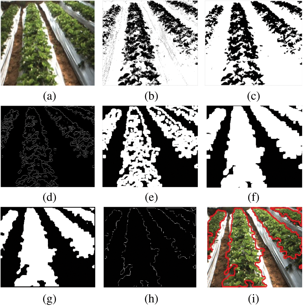
Figure 6: Extracting process of edge contours of crop rows (a) Original image (b) Binarized image (c) Filtered result (d) Edge extraction (e) Dilated image (f) Filled image (g) Eroded image (h) Edge contour image (i) Edges detected
3.3 Confidence-Based Dense Image
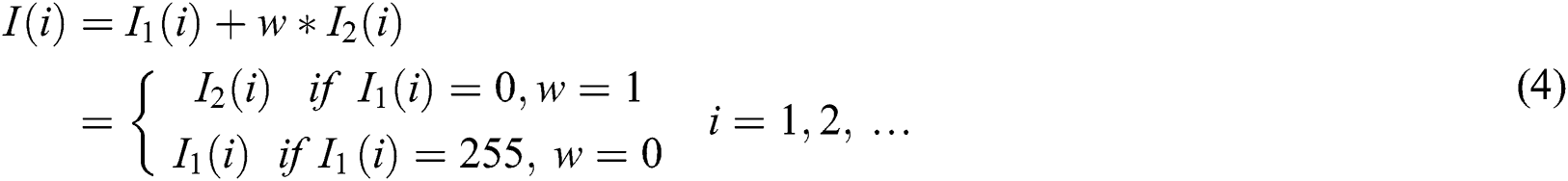
To make sufficient use of the crop row growth information, in this paper, we fuse the height and the edge information to produce the adaptive navigation parameters for an agricultural robot by using Eq. (4) (the fused image is called a confidence dense image), as shown in Fig. 7d. During the fusion, if the grayscale value of a point in the fused image exceeds 255, it will be set to 255. In Eq. (4),  is the ith pixel grayscale value of the binarized edge image (corresponding to a 2D image);
  is the value of the elevation image (corresponding to a 3D image), ranging from 0 to 255; w is defined as a fusing factor that can integrate the grayscale value of the fusing image.
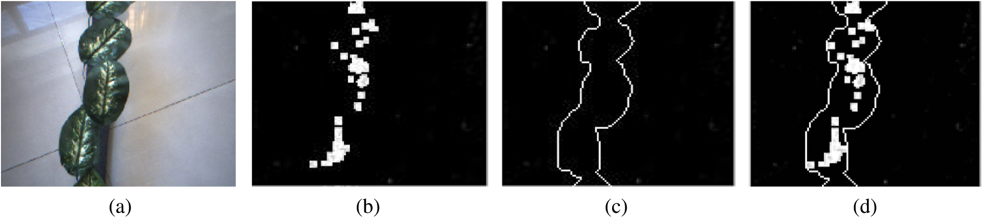
Figure 7: Process of producing Confidence-based dense image (a) Original image (b) Elevation image (c) Crop edge image (d) Confidence dense image
The confidence dense image proposed in this paper can be considered as the probability of a crop plant occurring in the corresponding position in a row image. If the grayscale value of a certain pixel point in the crop row image is bigger than the other, the probability of this point regarded as the crop row point is relatively higher. However, if the grayscale value of the point is smaller than the other, it will have a relatively smaller probability as a crop row point (the threshold value set is  , as shown in Eq. (3). At the same time, the black pixels inside the crop may be weeds, or crops that do not reach the set threshold height. In this case, the binarized edge image can be used to obtain navigation information and the elevation image can be used to improve the robustness of the recognition of the irregular crop rows. Therefore, the confidence-based dense image can be used to reliably extract the parameters needed for the navigation system of the smart agricultural robot.
In the experiments the agricultural robot used a four-wheel differential steering method. The steering model is shown in Fig. 8a. The parameters  and
and  represent the width and the length of the agricultural robot, respectively. The σ represents the steering angle. This is a typical structure model of a smart agricultural robot.
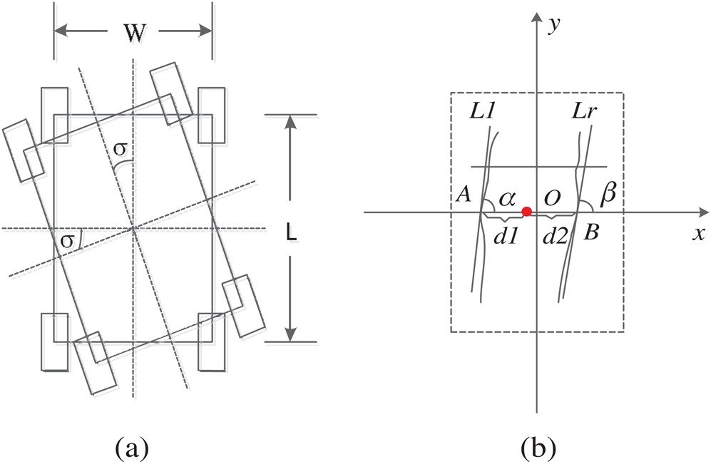
Figure 8: Steering model and diagram of navigation parameters (a) Steering model (b) Diagram of navigation parameters
In field environments, the edge contours of crop rows show different morphological features. This characteristic is not considered by existing conventional navigation algorithms that focus on extracting green crop-row lines. Moreover, when the crop plant is in its late growth stage, its edge contour information is more important than an extracted row line for guiding the smart agricultural robot to avoid crushing crop plant leaves. In this case, we have designed five basic adaptive navigation control network instructions, which are sent by the smart agricultural IoT system in this study and are based on the edge contour tangent lines to extract navigation parameters. This allows the smart agricultural robot to make adaptive posture adjustments during the automatic navigation process. In some green fields in particular, such as kale and cabbage, in the late growth stages, there is a need to consider the boundaries of crop leaves in the navigation information of the smart agricultural robot. Otherwise, the crushed crop leaves will affect the crop yield prediction and health status analysis when the robot works in the field to transmit the spectral image data to the cloud computing server [29].
Our navigation parameter extraction model is shown in Fig. 8b, in which we assume that the rectangle formed by the dotted line is a frame crop image in the computer buffer taken by a camera. The point O is regarded as a reference point marked red with the high density in x-coordinate direction, and is calculated by the white points from elevation images.  and
and  are tangent lines passing the two edges points A and B, respectively.
In Fig. 8b, the sign α denotes an angle between  and the x-axis, and
  denotes an angle between
  and the x-axis. The sign
  is a navigation control angle, being obtained by Eq. (5). The
  and
and  represent the distances from the reference point to the corresponding two edge points of a crop row, respectively. The sign d denotes a lateral distance of the agricultural robot relative to the reference point, as expressed by Eq. (6).

In Eq. (5), (x1,y1), (x2,y2) belong to  ; (x3,y3), (x4,y4) belong to
  .
.

Generally, the working status of a smart agricultural robot can be either straight moving status or turning status. Straight moving status is easy to steer; the turning statuses are relatively complex. Thus, the turning statuses are divided into four cases: Left turning, right turning, right turn with straight moving, and left turn with straight moving. The corresponding statuses’ network instruction sets sent by the smart agricultural IoT system are expressed in Eq. (7–11), where  and dt are the thresholds corresponding to the navigation angle
  and the lateral distance
  . The threshold
  and dt are set to 35° and 15 cm, respectively.
The moving instructions are determined by the moving statuses of a smart agricultural robot in the field, which represent its basic moving steps as follows.
1) Instruction set of straight moving status
In this case, the distance between the left crop boundary and the wheel is roughly the same as that of the right boundary and the corresponding wheel. When the parameter d satisfies Eq. (7), the smart agricultural robot will enter the straight moving status.

2) Instruction set of right turning status
When Eq. (8) is satisfied, the agricultural robot will enter right turning status. This usually occurs in a situation in which the angle difference  between two tangent lines is relatively large. Therefore, the possibility of crops on the right of a frame image is higher.

3) Instruction set of right turn with straight moving status
When Eq. (9) is satisfied, the agricultural robot will turn right and go straight. In this case, the angle difference  between two tangent lines is relatively small, but the possibility of crops on the right is higher. Therefore, the agricultural robot needs to make a slight adjustment to the right, and then advances in a straight line.

4) Instruction set of left turning status
When Eq. (10) is satisfied, the agricultural robot will turn left. This usually occurs in a situation in which the angle difference  between two tangent lines is relatively large. Therefore, the possibility of crops on the left of a frame image is higher.

5) Instruction set of left turn with straight moving status
When Eq. (11) is satisfied, the agricultural robot will turn left and move in a straight line. In this case, the angle difference  between two tangent lines is relatively small, but the possibility of crops on the left of a frame image is high. Therefore, the agricultural robot needs to make a slight adjustment to the left and then advances in a straight line.

When the serial image data from the binocular cameras in the data acquisition layer are processed in real time in the cloud computing layer, the instruction sets obtained can be transmitted in real time to the controller through the transmission layer to control the corresponding actual movements of the smart agricultural robot.
4 Experimental Results and Discussions
In the experiments, we used the Bumblebee2 binocular vision system (Model BB2-03S2C-60, Canada) and a smart agricultural robot (manufactured in Shanghai, China). The agricultural robot is 107 cm long and 82.3 cm wide, with a tire width of 15 cm. These specifications are designed according to the field operation requirements for smart agricultural robots in North China. All program codes of image data processed were run in the C++ environment on a computer with an Intel Core2 Duo CPU and 1.96 GB of RAM to test the adaptive navigation algorithm proposed in this study, which can only meet the low-speed requirements of less than 0.5 m/s of the smart agricultural robot. These specifications will need to be extended further to the cloud computing layer of the smart agricultural robot navigation IoT system designed in this study to speed up the image data processing and accomplish more intelligent operations in fields. The navigation parameter extraction and motion instruction sets designed were validated in the simulation experiments by designing  and
and  type of moving paths, as shown in Fig. 9a and 9b. The moving trails of the smart agricultural robot were recorded by putting black toner on the middle of its tires. Then we manually recorded the data of the moving trails and the planning paths. In Fig. 9c and d, the black curves represent actual moving trails of the smart agricultural robot; the red curves represent the edge contours of the simulated row.
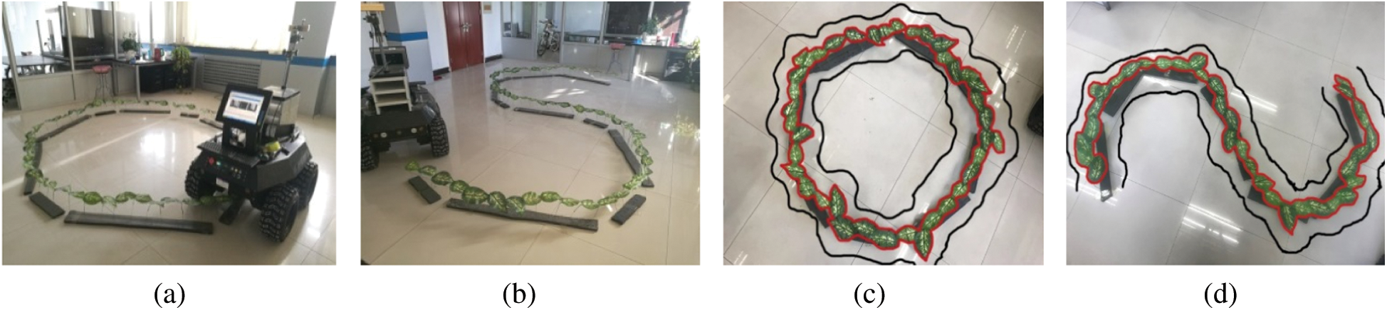
Figure 9: Display of planning path and moving trails (a) O-type path (b) S-type path (c) O-type moving trail (d) S-type moving trail
In the experiments, the smart agricultural robot did not crush the simulated crop plant leaves when the navigation parameter d satisfied 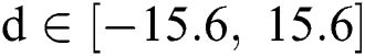 cm, according to the crop row space and its width. The results from running the experiment six times are shown in Fig. 10a and 10b, in which the actual measuring value of
  ranges from −10 cm to 10 cm. This means that the values of the parameter
  in the experiments all fell into the required range, indicating that the smart agricultural robot could normally move along a simulated crop row edge contour without crushing its leaves.
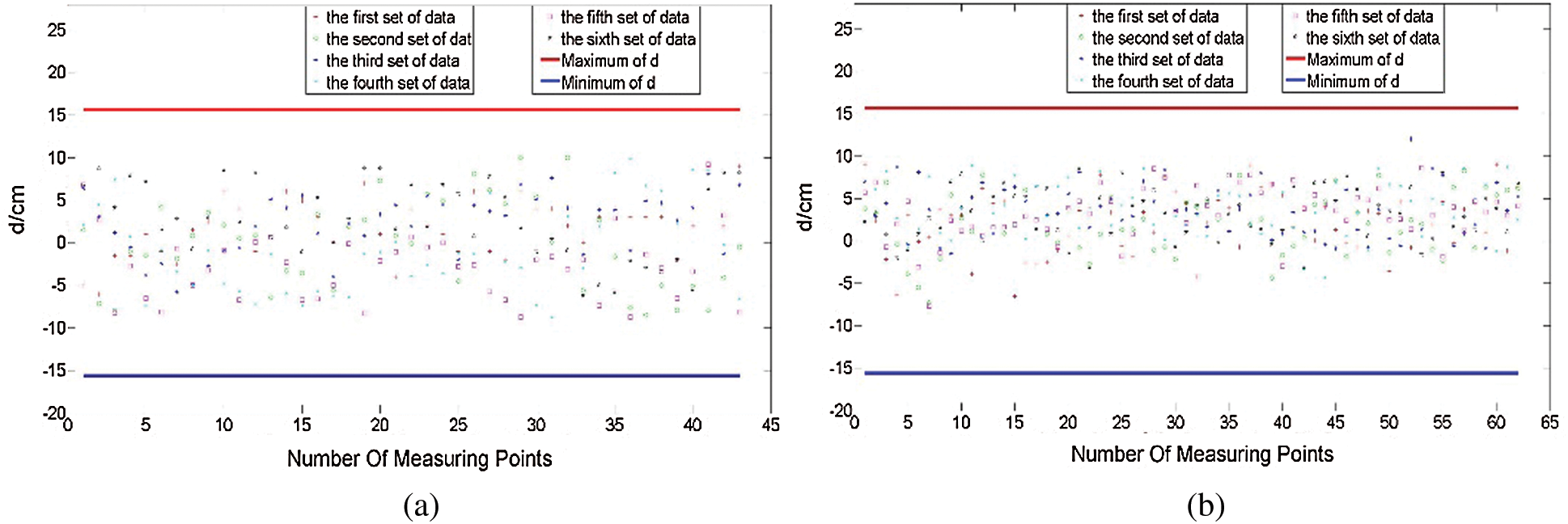
Figure 10: Measured d of the two moving trails (a) d values of O-type trail (b) d values of S-type trail
To highlight the edge-based navigation method proposed in this study, the contrast experiments based on the maximum density row-line detection without edge information proposed in the literature [30] (the speed of the agricultural robot is also less than 0.5 m/s) were conducted in the same experimental path of O-type and S-type. The motion trails of the smart agricultural robot are shown in Fig. 11a and 11b. The black lines are the robot’s actual paths. The values of d were obtained by conducting the experiments six times, as shown in Fig. 11c and 11d.
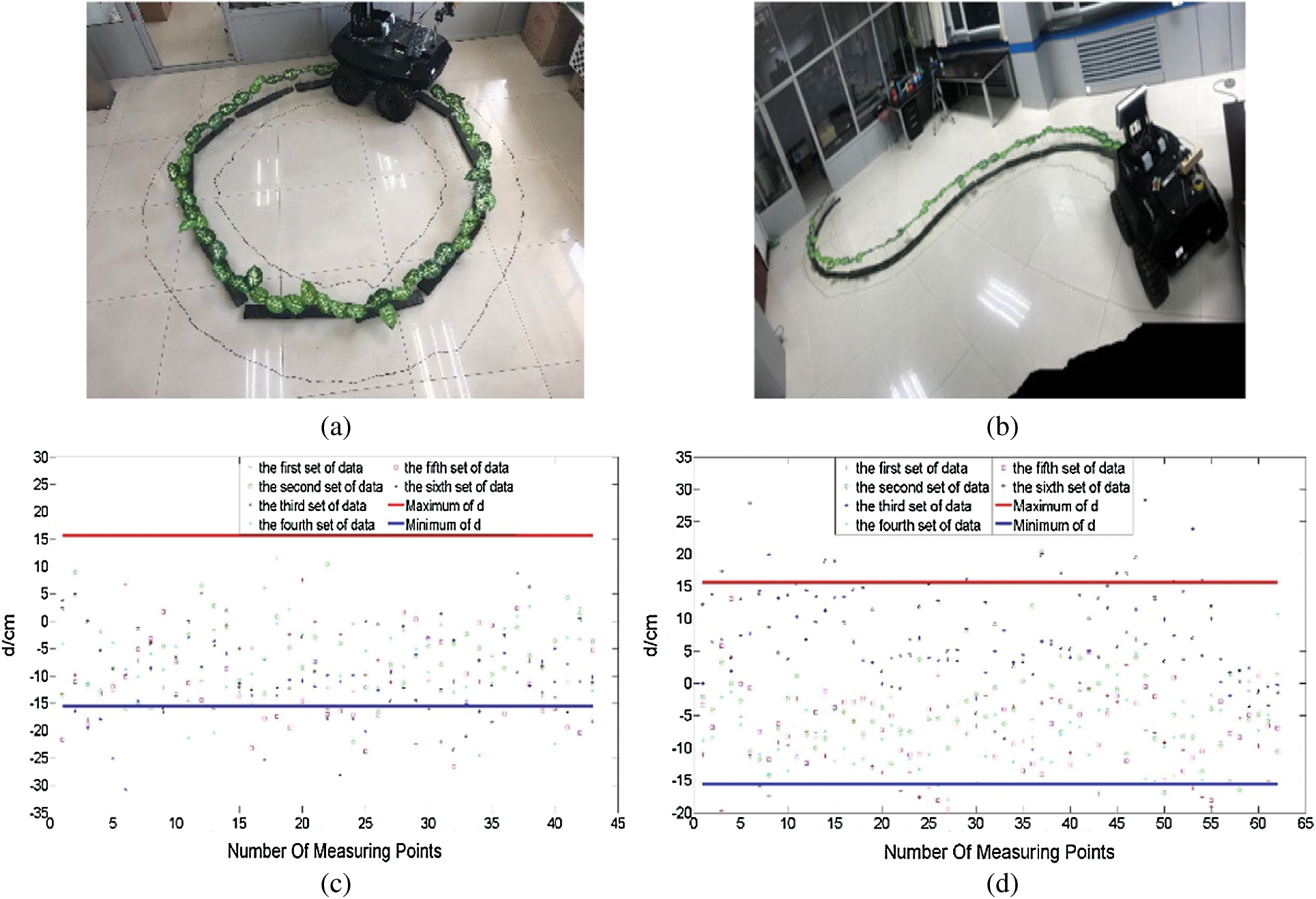
Figure 11: Comparison of experimental results of different methods proposed in [30] (a) O-type path (b) S-type path (c) d values of O-type trail (d) d values of S-type trail
In the experimental results, some d values located above the red line or below the blue line exceed the required range, indicating that the simulated crop leaves in these points’ positions were crushed by the smart agricultural robot. Their means are 7.18 cm and 8.00 cm, with standard deviations of 4.67 cm and 5.82 cm. However, the experimental results from running our algorithm, as shown in Fig. 10, show that these situations of crushed crops never occur, with the means being only 3.85 cm and 3.00 cm, with corresponding standard deviations of only 2.44 cm and 1.92 cm.
Furthermore, we fit a curve equation of the steering angle σ and the navigation angle θ of the agricultural robot by using Matlab14 function Fourier, shown in Eq. (12), where the edge contour points parameters  are taken every 4 cm in an O-type planning path, the parameter
  is obtained by implementing our algorithm procedure, and the parameter
  is obtained manually.

In this experiment, the coefficients of the equation are shown in Tab. 1.
Table 1: Function parameter values
To further validate the above function, the testing process was performed in an S-type planning path. The results are shown in Fig. 12.
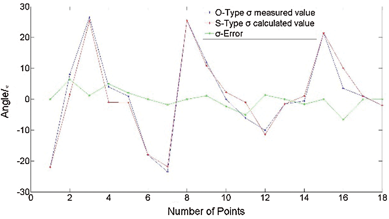
Figure 12: Comparison of the manually measured σ and σ, as calculated by Eq. (12)
Due to the irregularity of crop rows in their late growth stages, the smart agricultural robot needs to adjust its moving posture during navigation. Therefore, the fitting equation is nonlinear, with R2 of 0.96. The absolute mean of turning angle error is 0.7° with an absolute standard deviation of 1.5°, indicating that our navigation algorithm for the agricultural robot has good turning performance. Although the experimental results are obtained in simulated environments, without loss of generality, our proposed algorithm has fully fused the edge and height information of real crop rows. It can then be embedded into the smart agricultural IoT, and it will lay down a foundation in the vision navigation application field of smart agricultural robots.
To achieve automatic navigation in a smart agricultural robot, we proposed an adaptive vision navigation algorithm, which can be embedded into the smart agricultural robot IoT system we designed. The adaptive visual navigation algorithm can fuse the edge contour and height information of crops to extract the navigation parameters of the smart agricultural robot. The navigation network instruction sets designed for this study were successfully validated according to the moving statuses of the smart agricultural robot in the field. The simulated experimental results show that the smart agricultural robot can autonomously advance along S-type and O-type planning paths without crushing the leaves of the crop plant when its speed is less than 0.5 m/s, with an absolute mean of turning angle error of 0.7° and an absolute standard deviation of 1.5°. Our work provides a valuable reference for further practical application of the smart agricultural robot in responding to green crops in different growth periods.
Acknowledgement: We are grateful to the National Natural Science Foundation of China for its support, and to all reviewers for their work and patience.
Funding Statement: This study has been financially supported by the National Natural Science Foundation of China (No. 31760345). The author who received the grant is Zhibin Zhang. The URL for the sponsor’s website is http://www.nsfc.gov.cn/.
Conflicts of Interest: All authors declare that we have no conflicts of interest to report regarding the present study.
References
1. B. Kakillioglu, K. Ozcan and S. Velipasalar. (2016). “Doorway detection for autonomous indoor navigation of unmanned vehicles,” in IEEE Int. Conf. on Image Processing, Phoenix, AZ, pp. 25–28.
2. G. Zhou, J. Yuan, I. L. Yen and F. Bastani. (2016). “Robust real-time UAV based power line detection and tracking,” in IEEE Int. Conf. on Image Processing, Phoenix, AZ, pp. 25–28.
3. N. Efthymiou, P. Koutras, P. P. Filntisis, G. Potamianos and P. Maragos. (2018). “Multi-view fusion for action recognition in child-robot interaction,” in IEEE Int. Conf. on Image Processing, Athens, Greece, pp. 7–10.
4. Z. G. Gao, S. X. Xia, Y. K. Zhang, R. Yao, J. Q. Zhao et al. (2018). , “Real-time visional tracing with compact shape and color feature,” Computers, Materials & Continua, vol. 55, no. 3, pp. 509–521.
5. S. Hiremath, F. K. V. Evert, C. T. Braak, A. Stein and G. V. D. Heijdena. (2014). “Image-based particle filtering for navigation in a semi-structured agricultural environment,” Biosystems Engineering, vol. 121, pp. 85–95.
6. G. Zaidner and A. Shapiro. (2016). “A novel data fusion algorithm for low-cost localisation and navigation of autonomous vineyard sprayer robots,” Biosystems Engineering, vol. 146, pp. 133–148.
7. J. P. Vasconez, G. A. Kantor and F. A. A. Cheein. (2019). “Human−robot interaction in agriculture: A survey and current challenges,” Biosystems Engineering, vol. 179, pp. 35–48.
8. X. Y. Gao, J. H. Li, L. F. Fan, Q. Zhou, K. M. Yin et al. (2018). , “Review of wheeled mobile robots’ navigation problems and application prospects in agriculture,” IEEE Access, pp. 1.
9. B. W. Wang, W. W. Kong, H. Guan and N. N. Xiong. (2019). “Air quality forcasting based on gated recurrent long short term memory model in internet of things,” IEEE Access, vol. 7, no. 1, pp. 69524–69534.
10. P. M. Blok, K. V. Boheemen, F. K. V. Evert, J. IJsselmuiden and G. H. Kim. (2019). “Robot navigation in orchards with localization based on particle filter and Kalman filter,” Computers and Electronics in Agriculture, vol. 157, pp. 261–269.
11. Q. Zhang, M. E. S. Chen and B. A. Li. (2017). “A visual navigation algorithm for paddy field weeding robot based on image understanding,” Computers and Electronics in Agriculture, vol. 143, pp. 66–78.
12. B. Fernandez, P. J. Herrera and J. A. Cerrada. (2018). “Robust digital control for autonomous skid-steered agricultural robots,” Computers and Electronics in Agriculture, vol. 153, pp. 94–101.
13. I. D. García-Santillán, M. Montalvo, J. M. Guerrero and G. Pajares. (2017). “Automatic detection of curved and straight crop rows from images in maize fields,” Biosystems Engineering, vol. 156, pp. 61–79.
14. S. W. Searcy and J. F. Reid. (1986). “Detecting crop rows using the Hough transform,” in ASAE Annual Meeting. St, Joseph, MI.
15. H. T. SoGaard and H. J. Olsen. (2003). “Determination of crop rows by image analysis without segmentation,” Computers and Electronics in Agriculture, vol. 38, no. 2, pp. 141–158.
16. T. Bakker, H. Wouters, K. van Asselt, J. Bontsema, L. Tang et al. (2008). , “A vision-based row detection system for sugar beet,” Computers and Electronics in Agriculture, vol. 60, no. 1, pp. 87–95.
17. X. Zhang, X. Li, B. Zhang, J. Zhou, G. Tian et al. (2018). , “Automated robust crop-row detection in maize fields based on position clustering algorithm and shortest path method,” Computers and Electronics in Agriculture, vol. 154, pp. 165–175.
18. M. Kise and Q. Zhang. (2008). “Development of a stereovision sensing system for 3D crop row structure mapping and tractor guidance,” Biosystems Engineering, vol. 101, no. 2, pp. 191–198.
19. D. Jiang, L. Yang, D. Li, F. Gao, L. Tian and L. Li. (2014). “Development of a 3D ego-motion estimation system for an autonomous agricultural vehicle,” Biosystems Engineering, vol. 121, pp. 150–159.
20. L. Comba, A. Biglia, D. R. Aimonino and P. Gay. (2018). “Unsupervised detection of vineyards by 3D point-cloud UAV photogrammetry for precision agriculture,” Computers and Electronics in Agriculture, vol. 155, pp. 84–95.
21. J. Zhang, L. He, M. Karkee, Q. Zhang, X. Zhang and Z. Gao. (2018). “Branch detection for apple trees trained in fruiting wall architecture using depth features and regions-convolutional neural network (R-CNN),” Computers and Electronics in Agriculture, vol. 155, pp. 386–393.
22. G. Ren, T. Lin, Y. Ying, G. Chowdhary and K. C. Ting. (2020). “Agricultural robotics research applicable to poultry production: A review,” Computers and Electronics in Agriculture, vol. 169, pp. 105216.
23. F. Y. Bu and X. Wang. (2019). “A smart agriculture IoT system based on deep reinforcement learning,” Future Generation Computer Systems, vol. 99, pp. 500–507.
24. L. Huang, F. P. Da and S. Y. Gai. (2019). “Research on multi-camera calibration and point cloud correction method based on three-dimensional calibration object,” Optics and Lasers in Engineering, vol. 115, pp. 32–41.
25. Y. Wang, F. Yuan, H. Jiang and Y. H. Hu. (2016). “Novel camera calibration based on cooperative target in attitude measurement,” Optik, vol. 127, no. 22, pp. 10457–10466.
26. H. Bay, T. Tuytelaars and L. Van-Gool. (2006). “SURF: Speeded up robust features,” in 9th European Conf. on Computer Vision, Graz, Austria.
27. D. M. Woebbecke, G. E. Meyer, K. Von-Bargen and D. A. Mortensen. (1995). “Color indices for weed identification under various soil, residue, and lightning conditions,” Transaction of the ASAE, vol. 38, no. 1, pp. 259–269.
28. D. C. Marr and E. C. Hildreth. (1980). “Theory of edge detection,” Proceedings of the Royal Society of London. Series B, Biological Sciences, vol. 207, no. 1167, pp. 187–217.
29. L. Wang, P. X. Wang, S. L. Liang, Y. C. Zhu and J. Khan. (2020). “Monitoring maize growth on the North China Plain using a hybrid genetic algorithm-based back-propagation neural network model,” Computers and Electronics in Agriculture, vol. 170, pp. 105–238.
30. S. L. Zhao and Z. B. Zhang. (2016). “A new recognition of crop row based on its structural parameter model,” IFAC-PapersOnLine, vol. 49, no. 16, pp. 431–438.
 | This work is licensed under a Creative Commons Attribution 4.0 International License, which permits unrestricted use, distribution, and reproduction in any medium, provided the original work is properly cited. |