Computers, Materials & Continua DOI:10.32604/cmc.2020.012448
Article

Automatic and Robust Segmentation of Multiple Sclerosis Lesions with Convolutional Neural Networks

H. M. Rehan Afzal1,2,*, Suhuai Luo1, Saadallah Ramadan1,2, Jeannette Lechner-Scott1,2,3, Mohammad Ruhul Amin3, Jiaming Li4 and M. Kamran Afzal5

1School of Electrical Engineering and Computing, University of Newcastle, Callaghan, NSW 2308, Australia
2Hunter Medical Research Institute, New Lambton Heights, NSW 2305, Australia
3Department of Neurology, John Hunter Hospital, New Lambton Heights, NSW 2305, Australia
4CSIRO Data61, Marsfield, NSW 2122, Australia
5School of Computer Science and Technology, Xiamen University, Xiamen, 361005, China
*Corresponding Author: H. M. Rehan Afzal. Email: c3249813@uon.edu.au
Received: 01 July 2020; Accepted: 24 July 2020

Abstract: The diagnosis of multiple sclerosis (MS) is based on accurate detection of lesions on magnetic resonance imaging (MRI) which also provides ongoing essential information about the progression and status of the disease. Manual detection of lesions is very time consuming and lacks accuracy. Most of the lesions are difficult to detect manually, especially within the grey matter. This paper proposes a novel and fully automated convolution neural network (CNN) approach to segment lesions. The proposed system consists of two 2D patchwise CNNs which can segment lesions more accurately and robustly. The first CNN network is implemented to segment lesions accurately, and the second network aims to reduce the false positives to increase efficiency. The system consists of two parallel convolutional pathways, where one pathway is concatenated to the second and at the end, the fully connected layer is replaced with CNN. Three routine MRI sequences T1-w, T2-w and FLAIR are used as input to the CNN, where FLAIR is used for segmentation because most lesions on MRI appear as bright regions and T1-w & T2-w are used to reduce MRI artifacts. We evaluated the proposed system on two challenge datasets that are publicly available from MICCAI and ISBI. Quantitative and qualitative evaluation has been performed with various metrics like false positive rate (FPR), true positive rate (TPR) and dice similarities, and were compared to current state-of-the-art methods. The proposed method shows consistent higher precision and sensitivity than other methods. The proposed method can accurately and robustly segment MS lesions from images produced by different MRI scanners, with a precision up to 90%.

Keywords: Multiple sclerosis; lesion segmentation; automatic segmentation; CNN; automated tool; lesion detection

1  Introduction

Multiple Sclerosis (MS) is a common inflammatory neurological condition affecting the central nervous system (brain and spinal cord). It results in demyelination and axonal degeneration predominantly in the white matter of the brain [1]. Symptoms vary greatly from patient to patient, with common symptoms including weakness, balance issues, depression, fatigue, or visual impairment. Depending on the location of the inflammation, called plaques, different symptoms arise. These plaques can be detected by magnetic resonance imaging (MRI) but not computer tomography (CT). MRI is not only used for diagnosis but also considered to be the best tool to monitor progression of disease. Yearly MRI is nowadays considered standard of care. Detection rate of new lesions vary between radiologists from 64–82% [2]. As current MRI technologies only detect 30% of actual pathology [3], current research is focused on improvement of MRI techniques and analysis to detect lesions more accurately.

Radiologists use T1-w, T2-w and FLAIR sequences to detect inflammatory lesions and axonal damage but sensitivity depends on slice thickness and is laborious and time-consuming. T1-w, T2-w and FLAIR are different pulse sequences of MRI which are attained with different relaxation times. Automated segmentation and detection algorithms can overcome these issues. Significant advances have been made for the segmentation of medical imaging with the help of traditional machine learning techniques [4,5] and over the last few years advanced deep learning techniques made significant advancements in segmentation, detection, and recognition tasks. Several methods have been described for the automatic detection and segmentation of lesions in MRI of MS [6–8]. Some online challenges for the segmentation of lesions in MS, like International Symposium on Biomedical Imaging (ISBI) [9] and Medical Image Computing and Computer Assisted Intervention (MICCAI) [10] are providing a platform for researchers to showcase their innovations. These challenges not only provide MRI datasets but also provide the opportunity to compare different automated segmentation algorithms on the same cohorts. The need for such algorithms has arisen due to limited human capacity to analyse the large number of clinical images and the prohibitive increase in health care prices. For example, if there are more than 150 brain slices of a single MS patient and all slices have several lesions, it is nearly impossible to manually detect all lesions accurately. Machine learning and deep learning techniques can improve the detection rate of lesions and minimise analysis time, irrespective of the number of slices and lesions.

To cope with such type of issues, several algorithms have been proposed claiming good efficiency for the segmentation of MS lesions. These algorithms can be categorized into two main types, supervised and unsupervised [11]. After a detailed literature review, results indicate that supervised methods are more favoured and have an edge over unsupervised methods due to several reasons [12]. Unsupervised methods are not very popular for medical segmentation but have some promising results as well. Unsupervised methods mostly depend on the intensity of MR brain images where high intensities in the MRI are considered as outliers. Garcia-Lorenzo et al. [13] have published a specific example of such an unsupervised method that uses intensity distributions. Several other unsupervised methods like the one presented by Roura et al. [14] proposed a thresholding algorithm and Strumia et al. [15] presented a probabilistic algorithm. Tomas-Fernandez et al. [16] claimed that if we have additional information about the distribution of intensity and also know the expected location of normal tissue it could help to outline lesions more precisely. Sudre et al. [17] proposed an unsupervised framework in which no prior knowledge is needed to differentiate between the patterns of different abnormal images. They were able to detect such clusters that were abnormal in nature known as lesions, on clinical and simulated data. They segmented lesions restricted to white matter.

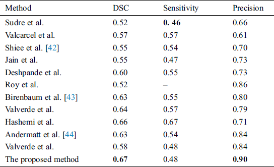
Supervised methods use templates consistent of MR images with manually segmented lesions from qualified radiologists. One of the best examples is of Valverde et al. [18], who proposed a cascaded network of two CNN. Our proposed algorithm also follows this principle of cascaded CNNs. Han et al. [19] also proposed 2 deep neural networks by teaching every network with mini batch and these two networks were communicated with each other to check which mini batch should be used for training purposes. They used different image datasets like CIFAR-10, CIFAR-100, and MNIST, etc., to check the robustness of their proposed network. One similar approach was proposed by Zhang et al. [20], who proposed deep mutual learning which is also called DML strategy. In this technique, instead of one-way transfer among students and a static teacher, students collaboratively learn and teach separately during the training. Valcarcel et al. [21] proposed an automatic algorithm for the segmentation of lesions which uses covariance features from regression. They also have taken part in a segmentation challenge and their results were based on a dice similarity coefficient (DSC) of 0.57 with a precision of 0.61. Jain et al. [22] proposed an automated algorithm in which they segmented white matter lesions as well as white matter, grey matter, and cerebro-spinal-fluid (CSF). Their method depended on prior knowledge of the appearance and location of lesions. Deshpande et al. [23] proposed a supervised based method with the help of healthy brain tissues and learning dictionaries. They also used a complete brain in which CSF, grey matter and white matter were included. They claimed that the dictionary learning technique was superior while performing lesions and non-lesions patches. For every class, their method automatically adapted the dictionary size according to the complexity. One more supervised approach was proposed by Roy et al. [24]. They proposed a 2D patch-based CNN including two pathways, which accurately and robustly segmented the white matter lesions. After the convolutional pathway, they didn’t use fully connected layer but again used another pathway of convolutional layers for the prediction of the membership function. They claimed that it was much faster as compared to fully connected layer. Brosch et al. [25] suggested an approach to segment the whole brain with the help of 3D CNNs and Hashemi et al. [26] presented a novel method by implementing a 3D patch wised CNN. It used a densely connected network idea. One latest and best method in this group of CNNs is of Valverde et al. [27]. They have written two papers for the segmentation of lesions. In the first paper, they proposed a 3D patch-based approach in which two convolutional networks were used. The first network was able to find possible lesions whereas the second network was trained to remove misclassified voxels that got from the first network. While in the second paper, they examined the intensity domain effect on their previously CNN based proposed method. They won the ISBI segmentation challenge. All these methods described in this section, used the same parameters as DSC, precision, and sensitivity to check the accuracy. These methods are compared with the proposed method in Tab. 4.

Table 4: Comparison of the proposed method with state-of-the-art methods using ISBI dataset

The marvelous development of deep learning especially CNNs has revolutionized progress in the medical field. CNNs are helping with segmentation, detection and even prediction of diseases [28]. Contrary to traditional machine learning techniques that require handcrafted features, deep learning techniques can learn features by themselves [29] and know how to do fine tuning according to the input data which is a remarkable achievement. These methods have excellent accuracy. Literature is accumulating online for deep learning medical imaging. There are several advantages of CNNs which compromise two main features. First, it doesn’t need handcrafted features and can handle 2D and 3D patches and learn features automatically. Secondly, convolutional neural networks can handle very large datasets even within a limited time span. This achievement is due to advancement in graphic processing units (GPUs) which can help us to train our algorithm within a portion of the time. So, CNNs with the help of GPUs have remarkably progressed the medical field to solve complex problems.

Due to deep learning accuracy and achievements, we proposed a novel deep learning-based architecture which segments MS lesions accurately and robustly. The proposed method follows the principle of two convolutional neural networks in which first CNN finds the possible lesions and then second CNN rectifies the false positives and gives better results with regards to accuracy and speed. Our algorithm uses parallel convolutional pathways where the fully connected (FC) layer is replaced with CNNs, similar to the approach of Ghafoorian et al. [30]. The replacement of the FC layer with CNNs not only increases the speed but is also much accurate. The reason for the increment of speed is due to the removal of FC layer as we know that FC layer use memory and we are still not sure how many layers are needed at the output. Several recent articles [31–37] may be read for better understanding of deep learning techniques.

In the proposed algorithm, three MRI sequences, T1-w, T2-w, and FLAIR are used as input for CNNs and then concatenated. T1-w and T2-w only are used to remove artifacts of MRI. Fig. 1 shows the general diagram of the proposed method. Moreover, a detailed description of the proposed architecture is provided in Section 3.2 and illustrated in Fig. 2.

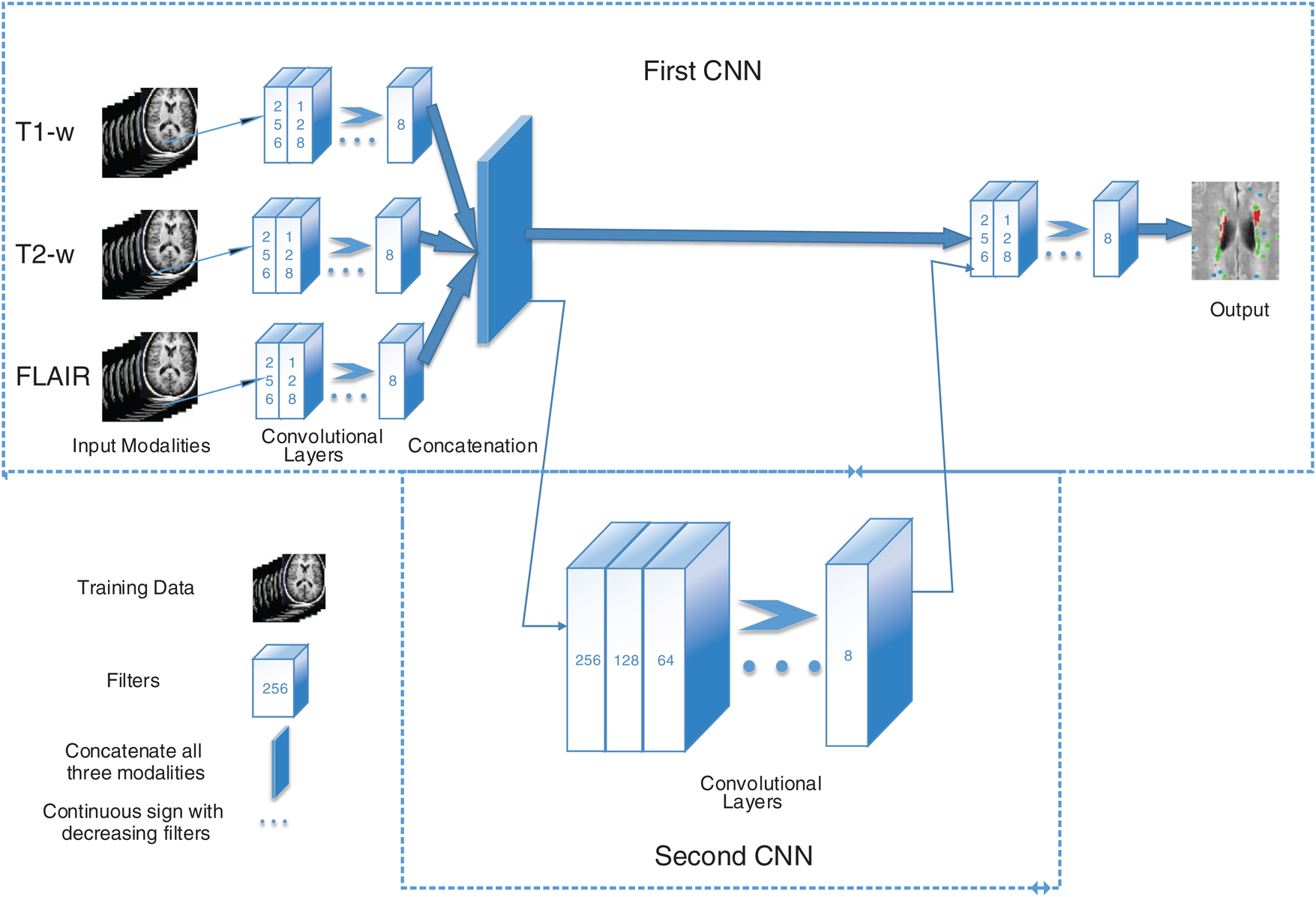
Figure 1: The general structure of the proposed method. First CNN consists of 6 convolutional layers with a decreasing number of filters from 256 to 8. Every filter has a size of 3 × 3 and 5 × 5 respectively. For example, the first layer has 256 filters with size 5 × 5, and then 128 filters with size 3 × 3 and so on. Three sequences have been used as inputs; T1-w, T2-w, and FLAIR. The second CNN is used as a parallel pathway to reduce the false positive

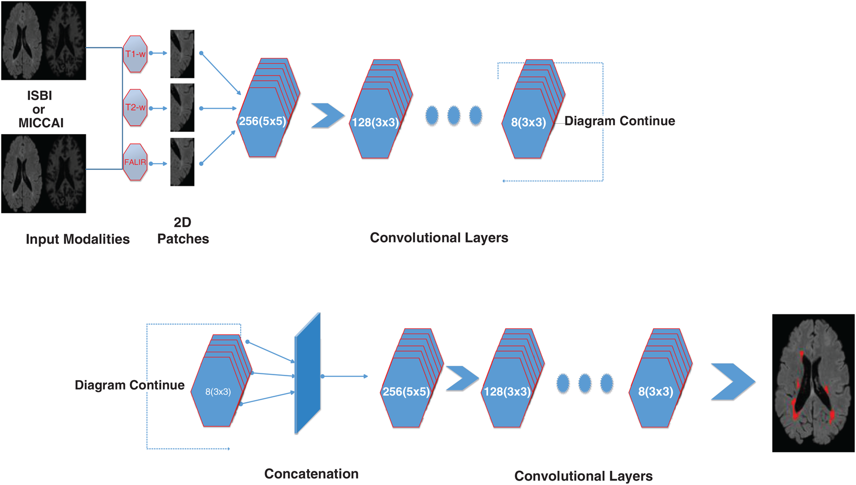
Figure 2: Detailed illustration/internal structure of the proposed method earlier shown in Fig. 1. At input two datasets are used (ISBI and MICCAI). Then 2D patches are obtained from all three sequences including T1-w, T2-w, and FLAIR. Then passed from the convolutional pathway of 6 layers by decreasing the number of filters from 256, 128, 64 to 8. Every filter has or a 3 × 3 size or 5 × 5 size alternatively. For example, the first layer has 256 filters with size 5 × 5 and then 128 filters with size 3 × 3 and so on

2  Data/Material

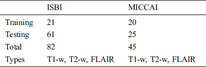
For the evaluation of the proposed method, two publicly available datasets are used. These two datasets ISBI and MICCAI are available for challenge purposes also. ISBI dataset consists of 82 scans in total, where 21 scans of 5 subjects are available for training purposes and already preprocessed with several steps like skull stripping, denoising, bias correction, and co-registration. These 5 subjects have 4 time points and one subject having 5 time points with a gap of approximately 1 year. These 21 scans are provided for training purposes only. For testing purposes, 61 scans are provided from 14 subjects.

For all scans, three different sequences T1-w, T2-w, and FLAIR are provided with manual annotations of the experts. The second dataset is composed of 45 scans where 20 scans are available for training which are attained at the University of Carolina (UNC) from a 3T Alegra scanner and Children’s Hospital Boston (CHB) from a 3T Siemens scanner. 25 scans are provided for testing purposes. For a better understanding of what we used for evaluation, all these details are tabulated in Tab. 1.

Table 1: ISBI and MICCAI datasets

3  Method

3.1 Preprocessing

The two provided datasets were already pre-processed as provided, and this included: skull stripping, image denoising, intensity normalization and image registration. Skull stripping was performed using a Brain Extraction Tool (BET) by Salehi et al. [38], while intensity normalization was implemented by N3 intensity normalization by Leger et al. [39]. Image denosing was performed with Gaussian pre-smoothing filters. Rigid registration was performed using Functional Magnetic Resonance Imaging of the Brain (FMRIB) Linear image registration (FLIRT).

3.2 CNN Architecture

Before training, all T1-w, T2-w, and FLAIR images were converted into 2D patches . The benefit of making 2D patches is to speed up the process. Results show that 2D patches are far better in speed and robustness compared to 3D patches. 3D patches need more memory, resulting in a slower speed. According to ISBI, dataset contains 1% lesions of total brain size, so we used large patches like 25 × 25 or 35 × 35 (2D patches). It helped us to reduce the balancing issue, which works better with 2D patches. According to Ghafoorian et al. [30], larger patches produce more accurate results. These 2D patches are made so that p is the size of two dimensions and these are stacked in an array containing where is “input modalities”, in our case .

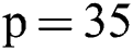
Due to the increased popularity of cascaded convolutional neural networks, the proposed method was also implemented with the help of such networks. The first network finds the possible true positives of required lesions, then the second network refines the results of already segmented lesions, and also decreases the false positives, which can be seen in Fig. 4, where (b) shows the manual segmentation of lesions, (c) shows the results of the first network (d) shows the results from the second network, and if we compare (c) and (d), it is clear that after the second network, false positives are decreased. After constructing 2D patches, these are passed through convolutional filter banks and then instead of fully connected layer, again convolutional filter banks are introduced for the prediction of the possible membership function. The reason for not using FC is that we are not sure how many layers are needed for prediction and the system might become too complex. We have applied the approach of GoogleNet and the recently proposed ResNet by He et al. [40], where they use fully convolutional layers instead of FC layer. Traditional CNNs use fully connected (FC) layer for the prediction of the probability of membership function, but the proposed method uses convolutional filters bank for several reasons. The main reason of not using FC layer is parameters complexity. Mostly we are not sure, how many parameters are needed to handle the features from previously convolved filters, which results, unused free parameters. The consequences may be overfitting.

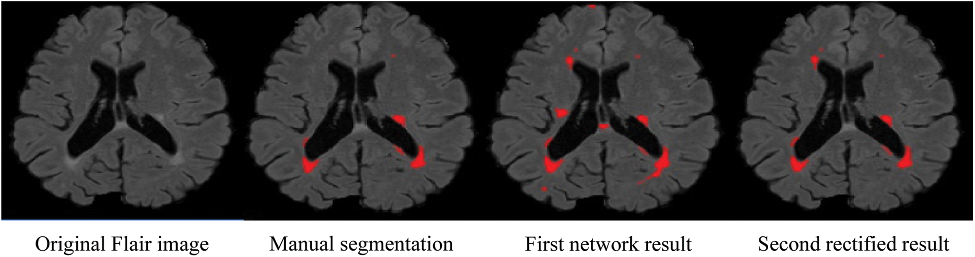
Figure 4: False positive comparison

The second reason for not using FC layer is that it can increase the time for prediction even using GPU. Because there are hundreds of slices for one scan and when slices are converted to patches, resulting in numerous patches for calculations. Therefore, using FC layer can reduce the time for prediction. The internal architecture of the proposed method can be seen in Fig. 2. It consists of 6 layers of convolutional filters and every convolutional filer has max-pooling and rectified linear unit (ReLU). The objective of max pooling is to down-size or reduce the dimensions of output and discarding the unwanted features to make the system fast. ReLU is used here because it is a speedy activation function. 6 layers of convolutional filters consist of different sizes of filters. So, it can be seen that the first layer has 256 filters with a size of 5 × 5 and the proceeding filter consisted of 128 filters with size 3 × 3. Then the next convolutional layers have a decreasing number of filters, 64 filters with size 5 × 5, 32 filters with size 3 × 3, 16 filters with size 5 × 5, and then the last layer consists of 8 filters of size 3 × 3.

After convolving the 2D patches with these 6 convolution layers, the output is concatenated. Then the concatenated output is passed again through parallel implemented convolutional filters bank for prediction purposes. Here we used small filter sizes like 3 × 3 and 5 × 5 for the convolution function. Small filter size is better as compared to big filters because a small filter can help to find the exact boundaries of lesions and train well for segmentation purposes. At the input, we have made 2D patches of three available modalities to speed up the process, and also to improve training. Patch size is denoted by , where is set to a different size and gathers results. For experiments, first, we started from small patches then we increased the size of patches. After reaching size 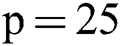, the outcome improved.

Valverde et al. [27] use small patches but they have good results, the reason is that they use a balanced training dataset. The training dataset consists of the voxels with lesion and also without lesions. This gives good results for smaller patches, but the drawback is that it consumes more time and is computationally expensive. Roy et al. used large patches. We also adopted large patches since we don’t need balanced training. Large patches contain large area which includes voxels with lesions and also without lesions. We only use those large patches which have lesion label as a center pixel. These large patches have an area “with lesion” and “without lesion”. It means all lesion patches with center voxel with lesion labels are selected. It not only speeds up the system but also makes it applicable for real applications due to less computations.

Therefore, we tried patch size 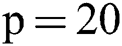, , and received good results as mentioned in the evaluation Section 4. Also, 3 modalities T1-w, T-2 w, and FLAIR are taken as input. The reason for taking 3 modalities is that, FLAIR is mainly used for segmentation purposes whereas the other 2 modalities T1-w and T2-w are used to reduce artifacts and help us to reduce false positives which are mentioned in Fig. 4. The comparison of one modality versus three modalities is shown in Fig. 5. The results show that when three modalities are used, MRI artifacts can be reduced greatly. The exact implementation details are discussed in Section 4.1.

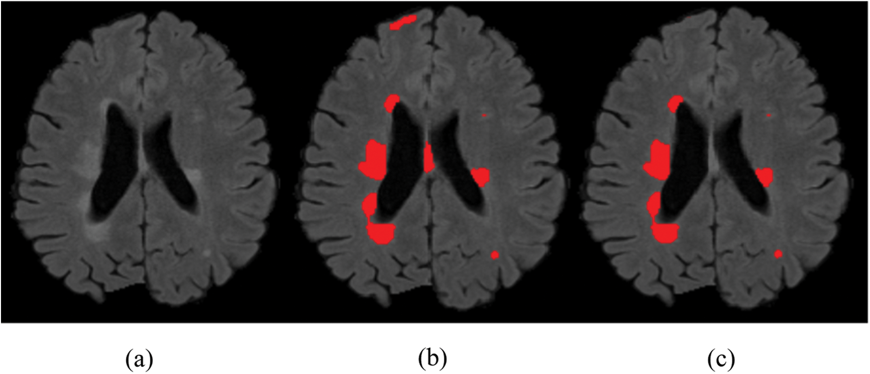
Figure 5: Comparison between 1 modality and 3 modalities. (a) Original image. (b) 1 modality. (c) 3 modalities

3.3 Evaluation Metrics

For evaluation purposes, two datasets ISBI and MICCAI have been used. For comparison, different state-of-the-art methods are compared, which are described in detail in Section 4.4. The evaluation is performed with the following metrics described below by comparing the performance against the human experts. The different metrics are sensitivity, precision and dice similarity coefficient.

3.3.1 Sensitivity

The sensitivity of the method can be calculated in terms of lesions true positive rate (LTPR) between automated segmentation and manual annotations of lesions

where denotes the correctly segmented lesions and also called true positive where is false negative or missed lesion region candidates.

3.3.2 Precision

Precision is considered as false discovery rate or lesions false positive rate (LFPR) between automatically segmented lesions and manually annotated lesions and expressed as

Here denotes false positive or the lesions which are incorrectly classified as lesions.

3.3.3 DSC

The overall accuracy of % segmentation in terms of dice similarity coefficient (DSC) between automated segmentation masks and manual annotated lesions area can be defined as

4  Results

4.1 Implementation Details

The proposed method is implemented using python language with Keras and TensorFlow due to open source and comprehensive libraries for machine learning. Results were taken at 20 epochs. 2.7 GHz Intel Xeon Gold (E5-6150) processor is used with 32 GB memory of Nvidia GPU. Data was divided into two parts: a training set and validation set, occupying 80% and 20% respectively. Best results were obtained by running 20 epochs for training set with a learning rate of 0.0001 and using the optimizer of Kingma et al. [41]. We have used early stopping with patience = 10, as in our case, we observed the best results at 20 epochs. The batch size was set to 128. It took 2 h and 16 min for training and just 15 s on average for testing or segmenting the lesions from an unseen image.

4.2 MICCAI Dataset

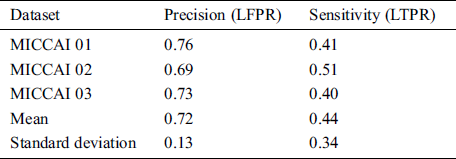
MICCAI dataset provides three sequences T1-w, T2-w, and FLAIR which we need, for our proposed algorithm. These modalities are input at the proposed CNN pathway and results were obtained by using evaluation metrics mentioned in Section 3.3. The proposed method has two pipelines CNN. First, dataset is converted into patches before input to proposed CNN, which increases the pseed of training and validation. Then these patches are divided into 80:20 strategy for the training set and validation, respectively. While making patches for the training set, whole patches were divided into two parts, where 80% patches were used for the training set and remaining patches, 20% were used for validation purposes. For example, when the patch size was 25 × 25, the total number of generated patches were 242775. From these total patches, 194220 were used for the training set and 48555 samples were used for validation. Tab. 2 shows the three results for the testing of MICCAI by using different factors like LTPR and LFPR. First three scan’s results of MICCAI 01,02 and 03 are shown below.

Table 2: MICCAI dataset evaluation results by using different metrics LTPR & LFPR

4.3 ISBI Dataset

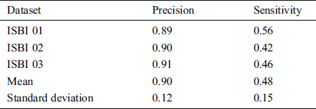
From the ISBI dataset, the results of the first 3 scans (ISBI 01, ISBI 02 and ISBI 03) are displayed in Tab. 3. ISBI results are evaluated on a qualitative and quantitative basis. Qualitative results can be seen in Fig. 3, whereas quantitative results have been shown in Tab. 3. Qualitative results in Fig. 3, show the original image, manually segmented image, proposed auto segmented image, and overlap of both manual and auto segmented images. Results show that our proposed method has good results for manual segmentation.

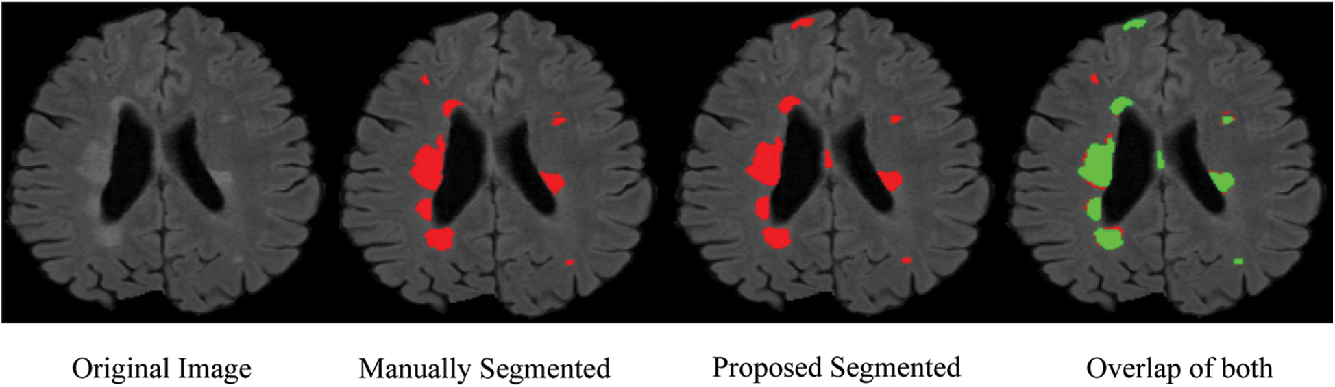
Figure 3: Qualitative results for ISBI dataset

Table 3: ISBI dataset evaluation results by using different metrics LTPR & LFPR

4.4 Comparison

In this section different state-of-the-art methods have been compared with the proposed method. All these methods used the same ISBI dataset and the same evaluation metrics as described in Section 3.3. Benchmark of the dataset was also provided on their website to compare the results. These benchmarks are manually annotated by the experts in the field of MS. These methods are evaluated by using various metrics like DSC, sensitivity, and precision. These results are tabulated as a mean of all results obtained with the help of the proposed method. The quantitative comparison of the proposed method with top rank existed methods is shown in Tab. 4. These values are extracted from the challenge website and some are extracted from their related publications. These results are considered best to date for the segmentation of lesions. The proposed method has more DSC as compared to all existed methods, where DSC is also called overall segmentation accuracy, described by ISBI challenge website. For the qualitative comparison with manually annotated lesions provided by ISBI are shown in Figs. 3, 4 and 7. To check the trade-off between sensitivity and precision, the receiver operating characteristic (ROC) curve is drawn for the proposed CNN approach on the ISBI dataset, shown in Fig. 6.

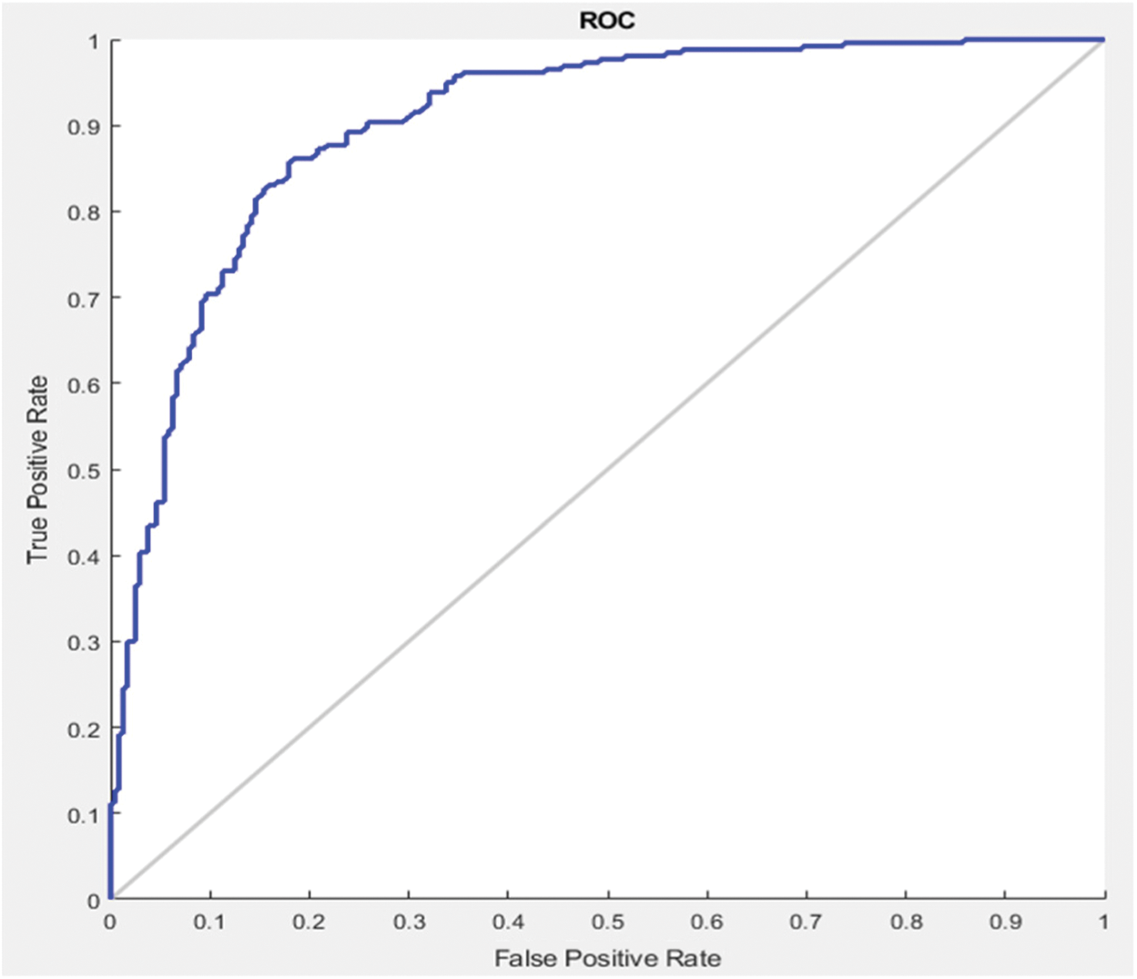
Figure 6: ROC curve between sensitivity and specificity

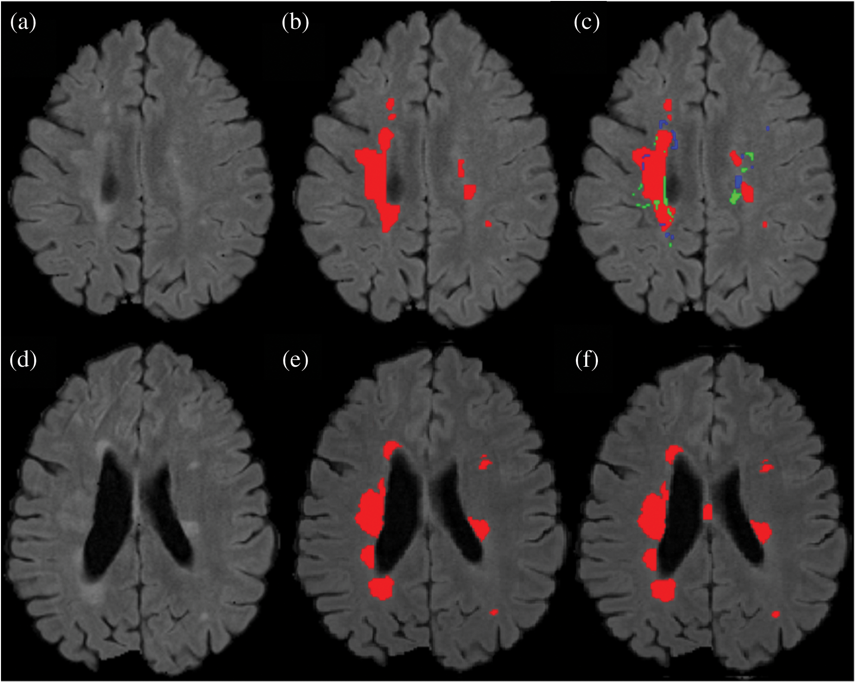
Figure 7: Comparison between the proposed method and manually segmented area/ground truth. (a) FLAIR image. (b) Manually segmented image. (c) auto segmented image / proposed method with true positive (red color), false positive (green color) and false negative (blue color). (d) FLAIR image of a second patient. (e) Manually segmented area of the second patient. (f) Auto/proposed segmented lesions of the second patient

Results show that the proposed method has excellent results not only in precision but also in speed and robustness as testing takes only 15 seconds on average for automatic segmentation of MS lesions. Some scans have less lesion load and some scans have more lesion load. Lesion load is referred as the volume or number of lesions. Average timing is calculated after calculating time for all available testing scans and then taking the average of all the values. In Fig. 7 the results are demonstrated qualitatively and can be compared with ground truth or manually segmented scans. The first row of Fig. 7 shows the results of the first tested scan and compared it with manually segmented masks. (a) shows the original FLAIR image and (b) displays a manual mask or ground truth. (c) is the automatic or proposed method that depicts different colors, where red is true positive, green is false positive, and blue is a false negative. Row 2 shows one more scan from the testing dataset. (d) is the original FLAIR image, (e) is manually segmented, and (f) is the automatic proposed method. After a qualitative comparison, it is clear that the proposed method segments lesions automatically and very accurately.

4.5 Robustness

To check the robustness of the proposed algorithm, the same architecture is used for the training of two different datasets like ISBI and MICCAI. Even both datasets are from different scanners. As mentioned in Section 2, three different MRI scanners like Siemens Aera 1.5T, Siemens Verio 3T, and Philips Ingenia 3T are used for these two datasets. However, the results are promising as mentioned in Tabs. 2, 3 and 4. Even considering that the images were taken at different time points with a gap of almost 1 year, the proposed method is stable for different types of parameters like DSC, precision, and sensitivity and also for different scanners and different types of patients.

5  Conclusion

Automatic lesion segmentation is required for diagnostic and monitoring purposes in MS. There is a desperate need for more efficacious and rapid lesion assessments. A six layers CNN is implemented with two cascaded pipelines. This network does not need fully connected (FC) layers but uses CNN for the prediction of the probability of membership function. It not only increases the speed but also decreases the false positive rate. The proposed method follows the supervised method principle which uses templates consisting of MR imaging with manually segmented masks from qualified radiologists. The proposed method accurately and robustly segmented MS lesions even for images from different MRI scanners with a precision of up to 90%. Therefore, this automated algorithm is able to help neurologists to segment lesions fully automatically without time wastage, improving disease monitoring.

However, the proposed algorithm has some limitations. While performing experiments, it was noted that if two lesions are very close or overlapping, sometimes the proposed algorithm is unable to segment precisely. Also, when lesions are near the cortex of the brain it was difficult to segment them. According to the ISBI dataset and expert opinion cortical lesions are difficult to detect. In future work, as new MRI sequences are being introduced, the proposed method will be checked with other sequences of large number of MRI scans. The proposed method will be also checked for different parameters, CNN layers, batch size, and different filters, etc.

Acknowledgement: We are thankful to Peter and Shiami (Radiologists at John Hunter Hospital) for manual segmentation of MRI scans.

Funding Statement: Thanks to research training program (RTP) of University of Newcastle, Australia and PGRSS, UON for providing funding. APC of CMC will be paid by PGRSS, UON funding.

Conflicts of Interest: The authors declare that they have no conflicts of interest to report regarding the present study.

References

This work is licensed under a Creative Commons Attribution 4.0 International License, which permits unrestricted use, distribution, and reproduction in any medium, provided the original work is properly cited.

References

1G. Macaron and D. Ontaneda. (2019), “Diagnosis and management of progressive multiple sclerosis. ,” Biomedicines, vol. 7, no. (3), pp, 56–78, .
2W. Wang, J. H. Van, M. A. Tacey and F. Gaillard. (2017), “Neuroradiologists compared with non-neuroradiologists in the detection of new multiple sclerosis plaques. ,” American Journal of Neuroradiology, vol. 38, no. (7), pp, 1323–1327, . [Google Scholar]
3A. Junker, J. Wozniak, D. Voigt, U. Scheidt, J. Ant el et al. (2020). , “Extensive subpial cortical demyelination is specific to multiple sclerosis. ,” Brain Pathology, vol. 30, no. (3), pp, 641–652, . [Google Scholar]
4H. Zhang, A. M. Valcarcel, R. Bakshi, R. Chu, F. Bagnato et al. (2019). , “Multiple sclerosis lesion segmentation with tiramisu and 2.5 D stacked slices. ,” in Int. Conf. on Medical Image Computing and Computer–Assisted Intervention, Shenzhen, China, pp, 338–346, . [Google Scholar]
5O. Commowick, F. Cervenansky and R. Ameli. (2016), “Multiple sclerosis lesions segmentation challenge using a data management and processing infrastructure. ,” in Proc. of MSSEG, Athènes, Greece, pp, 1–17, . [Google Scholar]
6R. McKinley, R. Wepfer, L. Grunder, F. Aschwanden, T. Fischer et al. (2020). , “Automatic detection of lesion load change in multiple sclerosis using convolutional neural networks with segmentation confidence. ,” NeuroImage: Clinical, vol. 25, no. (1), pp, 102–104, . [Google Scholar]
7C. Gros, B. Leener, A. Badji, J. Maranzano, D. Eden et al. (2019). , “Automatic segmentation of the spinal cord and intramedullary multiple sclerosis lesions with convolutional neural networks. ,” Neuroimage, vol. 184, no. (1), pp, 901–915, .
8P. A. Narayana, I. Coronado, S. J. Sujit, J. S. Wolinsky, F. D. Lublin et al. (2019). , “Deep learning for predicting enhancing lesions in multiple sclerosis. ,” Noncontrast MRI. Radiology, vol. 294, no. (2), pp, 10–61, . [Google Scholar]
9https://biomedicalimaging.org/2015/program/isbi-challenges. [Google Scholar]
10https://www.nitrc.org/projects/msseg. [Google Scholar]
11A. Carass, S. Roy, A. Jog, J. L. Cuzzocreo, E. Magrath et al. (2017). , “Longitudinal multiple sclerosis lesion segmentation: Resource and challenge. ,” NeuroImage, vol. 148, no. (1), pp, 77–102, . [Google Scholar]
12R. Zhang, F. Nie, Y. Wang and X. Li. (2019), “Unsupervised feature selection via adaptive multimeasure fusion. ,” IEEE Transactions on Neural Networks and Learning Systems, vol. 30, no. (9), pp, 2886–2892, . [Google Scholar]
13D. García-Lorenzo, S. Francis, S. Narayanan, D. L. Arnold and D. L. Collins. (2013), “Review of automatic segmentation methods of multiple sclerosis white matter lesions on conventional magnetic resonance imaging. ,” Medical Image Analysis, vol. 17, no. (1), pp, 1–18, . [Google Scholar]
14E. Roura, A. Oliver, M. Cabezas, S. Valverde, S. D. Pareto et al. (2015). , “A toolbox for multiple sclerosis lesion segmentation. ,” Neuroradiology, vol. 57, no. (10), pp, 1031–1043, . [Google Scholar]
15M. Strumia, F. R. Schmidt, C. Anastasopoulos, C. Granziera, G. Krueger et al. (2016). , “White matter MS-lesion segmentation using a geometric brain model. ,” IEEE Transactions on Medical Imaging, vol. 35, no. (7), pp, 1636–1646, . [Google Scholar]
16X. Tomas-Fernandez and S. K. Warfield. (2015), “A model of population and subject (MOPS) intensities with application to multiple sclerosis lesion segmentation. ,” IEEE Transactions on Medical Imaging, vol. 34, no. (6), pp, 1349–1361, . [Google Scholar]
17C. H. Sudre, M. J. Cardoso, W. H. Bouvy, G. J. Biessels, J. Barnes et al. (2015). , “Bayesian model selection for pathological neuroimaging data applied to white matter lesion segmentation. ,” IEEE Transactions on Medical Imaging, vol. 34, no. (10), pp, 2079–2102, . [Google Scholar]
18S. Valverde, M. Cabezas, E. Roura, S. González-Villà, D. Pareto et al. (2017). , “Improving automated multiple sclerosis lesion segmentation with a cascaded 3D convolutional neural network approach. ,” NeuroImage, vol. 155, no. (1), pp, 159–168, . [Google Scholar]
19B. Han, Q. Yao, X. Yu, G. Niu, M. Xu et al. (2018). , “Co-teaching: Robust training of deep neural networks with extremely noisy labels, ” in arXiv of Advances in Neural Information Processing Systems, Montreal, Canada: , pp, 8527–8537, . [Google Scholar]
20Y. Zhang, T. Xiang, T. M. Hospedales and H. Lu. (2018), “Deep mutual learning. ,” in Proc. of the IEEE Conf. on Computer Vision and Pattern Recognition, Salt Lake City, USA, pp, 4320–4328, . [Google Scholar]
21A. M. Valcarcel, K. A. Linn, S. N. Vandekar, T. D. Satterthwaite, J. Muschelli et al. (2018). , “MIMoSA: An automated method for intermodal segmentation analysis of multiple sclerosis brain lesions. ,” Journal of Neuroimaging, vol. 28, no. (4), pp, 389–398, . [Google Scholar]
22S. Jain, D. M. Sima, A. Ribbens, M. Cambron, A. Maertens et al. (2015). , “Automatic segmentation and volumetry of multiple sclerosis brain lesions from MR images. ,” NeuroImage: Clinical, vol. 8, no. (1), pp, 367–375, . [Google Scholar]
23H. Deshpande, P. Maurel and C. Barillot. (2015), “Classification of multiple sclerosis lesions using adaptive dictionary learning. ,” Computerized Medical Imaging and Graphics, vol. 46, no. (1), pp, 2–10, . [Google Scholar]
24S. Roy, J. A. Butman, D. S. Reich, P. A. Calabresi and D. L. Pham. (2018), “Multiple sclerosis lesion segmentation from brain MRI via fully convolutional neural networks. ,” ArXiv Preprint, arXiv no.1803.09172, . [Google Scholar]
25T. Brosch, L. Y. Tang, Y. Yoo, D. K. Li, A. Traboulsee et al. (2016). , “Deep 3D convolutional encoder networks with shortcuts for multiscale feature integration applied to multiple sclerosis lesion segmentation. ,” IEEE Transactions on Medical Imaging, vol. 35, no. (5), pp, 1229–1239, . [Google Scholar]
26S. R. Hashemi, S. S. Z. Salehi, D. Erdogmus, S. P. Prabhu, S. K. Warfield et al. (2018). , “Tversky as a loss function for highly unbalanced image segmentation using 3d fully convolutional deep networks. ,” ArXiv Preprint, arXiv no. 1803.11078, . [Google Scholar]
27S. Valverde, M. Salem, M. Cabezas, D. Pareto, J. C. Vilanova et al. (2019). , “One-shot domain adaptation in multiple sclerosis lesion segmentation using convolutional neural networks. ,” NeuroImage: Clinical, vol. 21, no. (10), pp, 16–38, . [Google Scholar]
28H. M. R. Afzal, S. Luo, S. Ramadan, J. Lechner-Scott and J. Li. (2018), “Automatic prediction of the conversion of clinically isolated syndrome to multiple sclerosis using deep learning. ,” in Proc. of the the 2nd Int. Conf. on Video and Image Processing, HongKong, China, pp, 231–235, . [Google Scholar]
29Y. LeCun, Y. Bengio and G. Hinton. (2015), “Deep learning. ,” Nature, vol. 521, no. (7553), pp, 436–444, . [Google Scholar]
30M. Ghafoorian, N. Karssemeijer, T. Heskes, I. W. V. Uden, C. I. Sanchez et al. (2017). , “Location sensitive deep convolutional neural networks for segmentation of white matter hyperintensities. ,” Scientific Reports, vol. 7, no. (1), pp, 1–12, . [Google Scholar]
31F. Yu, L. Liu, L. Xiao, K. L. Li and S. Cai. (2019), “A robust and fixed-time zeroing neural dynamics for computing time-variant nonlinear equation using a novel nonlinear activation function. ,” Neurocomputing, vol. 350, pp, 108–116, . [Google Scholar]
32M. Dua, R. Gupta, M. Khari and R. G. Crespo. (2019), “Biometric iris recognition using radial basis function neural network. ,” Soft Computing, vol. 23, no. (22), pp, 11801–11815, .
33M. Khari, A. K. Garg, R. G. Crespo and E. Verdú. (2019), “Gesture recognition of RGB and RGB-D static images using convolutional neural networks. ,” International Journal of Interactive Multimedia & Artificial Intelligence, vol. 5, no. (7), pp. 22–27, .
34D. Vishal, T. Bhavya and S. L. Puneet. (2020), “Micro-expression recognition using 3D–CNN. ,” Fusion Practice and Applications, vol. 1, no. (1), pp, 5–13, .
35F. Chen, W. H. Xu, C. Z. Bai and X. M. Gao. (2016), “A novel approach to guarantee good robustness of fuzzy reasoning. ,” Applied Soft Computing, vol. 41, pp, 224–234, .
36S. R. Zhou and B. Tan. (2020), “Electrocardiogram soft computing using hybrid deep learning CNN-ELM. ,” Applied Soft Computing, vol. 86, pp. 218–226, .
37J. M. Zhang, X. K. Jin, J. Sun, J. Wang and A. K. Sangaiah. (2018), “Spatial and semantic convolutional features for robust visual object tracking. ,” Multimedia Tools and Applications, vol. 79, no. (21–22), pp, 15095–15115, . [Google Scholar]
38S. S. M. Salehi, D. Erdogmus and A. Gholipour. (2017), “Auto-context convolutional neural network (auto-net) for brain extraction in magnetic resonance imaging. ,” IEEE Transactions on Medical Imaging, vol. 36, no. (11), pp, 2319–2330, . [Google Scholar]
39S. Leger, S. Lock, V. Hietschold, R. Haase, H. J. Bohme et al. (2017). , “Physical correction model for automatic correction of intensity non-uniformity in magnetic resonance imaging. ,” Physics and Imaging in Radiation Oncology, vol. 4, no. (1), pp, 32–38, . [Google Scholar]
40K. He, X. Zhang, S. Ren and J. Sun. (2016), “Identity mappings in deep residual networks. ,” in European Conf. on Computer Vision, Amsterdam, Netherlands, pp, 630–645, . [Google Scholar]
41D. Kingma and B. J. Adam. (2019), “A method for stochastic optimization. ,” in Int. Conf. on Learning Representations, New Orleans, USA, pp, 9–29, . [Google Scholar]
42N. Shiee, P. L. Bazin, A. Ozturk, D. S. Reich, A. Calabresi et al. (2010). , “A topology-preserving approach to the segmentation of brain images with multiple sclerosis lesions. ,” NeuroImage, vol. 49, no. (2), pp, 1524–1535, .
43A. Birenbaum and H. Greenspan. (2017), “Multi-view longitudinal CNN for multiple sclerosis lesion segmentation. ,” Engineering Applications of Artificial Intelligence, vol. 65, no. (1), pp, 111–118, .
44S. Andermatt, S. Pezold and P. C. Cattin. (2017), “Automated segmentation of multiple sclerosis lesions using multi–dimensional gated recurrent units. ,” in Int. MICCAI Brainlesion Workshop, Shenzhen, China, pp, 31–42, .