Computers, Materials & Continua DOI:10.32604/cmc.2020.012364
Article

Deep Feature Extraction and Feature Fusion for Bi-Temporal Satellite Image Classification

Anju Asokan1, J. Anitha1, Bogdan Patrut2, Dana Danciulescu3 and D. Jude Hemanth1,*

1Department of ECE, Karunya Institute of Technology and Sciences, Coimbatore, India
2Department of Computer Science, Alexandru Ioan Cuza University of laşi, laşi, Romania
3Department of Computer Science, University of Craiovo, Craiovo, Romania
*Corresponding Author: D. Jude Hemanth. Email: judehemanth@karunya.edu
Received: 27 June 2020; Accepted: 26 July 2020

Abstract: Multispectral images contain a large amount of spatial and spectral data which are effective in identifying change areas. Deep feature extraction is important for multispectral image classification and is evolving as an interesting research area in change detection. However, many deep learning framework based approaches do not consider both spatial and textural details into account. In order to handle this issue, a Convolutional Neural Network (CNN) based multi-feature extraction and fusion is introduced which considers both spatial and textural features. This method uses CNN to extract the spatio-spectral features from individual channels and fuse them with the textural features. Then the fused image is classified into change and unchanged regions. The presence of mixed pixels in the bitemporal satellite images affect the classification accuracy due to the misclassification errors. The proposed method was compared with six state-of-the-art change detection methods and analyzed. The main highlight of this method is that by taking into account the spatio-spectral and textural information in the input channels, the mixed pixel problem is solved. Experiments indicate the effectiveness of this method and demonstrate that it possesses low misclassification errors, higher overall accuracy and kappa coefficient.

Keywords: Remote sensing; convolutional neural network; deep learning; multispectral; bitemporal; change detection

1  Introduction

With the advances in sensor technology and availability of high resolution satellite imagery, monitoring of changes on earth’s surface has become easier. But the complexity of the bitemporal satellite images affect the accuracy of change classification. This mainly occurs due to the presence of brightness variations and variety of textural contrasts in satellite image which leads to mixed pixel problem. When the pixel region is composed of different areas that vary greatly with brightness and variations in texture and color, then the single value that represents the pixel may not represent a particular category. This problem is seen near the edges or along linear features where there are adjacent areas of contrasting brightness [1]. It is thus important to identify the variation in such image features to necessitate effective change detection and reduce the misclassification errors to improve the accuracy of change detection algorithm. The change map information is of utmost importance for classification map producers to improve the classification accuracy.

Change detection methods are divided into supervised and unsupervised techniques. The supervised techniques need some training samples for classification while the unsupervised technique can distinguish between the change and no-change regions without any preliminary information about the source image [2]. In supervised approach, by considering change detection as a binary classification problem, features are extracted from the image and then the classification is performed. For getting better results, many training samples with ground truth are given to the classifier which is known as pre-classification change detection. The advantage of this method is that complete information of the change can be obtained and gives higher accuracy than other techniques. But the need for larger training data limits the use of supervised change detection. The traditional change detection methods such as algebra-based Change Vector Analysis (CVA) [3], Principal Component Analysis (PCA) [4] and Multivariate Alteration Detection (MAD) [5] do not account for the spatial information in the image and are dependent on a single isolated pixel. Recently some deep models have been adopted for change detection in satellite imagery [6,7]. A dual channel CNN for spectral-spatial classification in hyperspectral images is presented in Zhang et al. [8]. This technique employs a 1D CNN for spectral feature extraction and a 2D CNN for extracting space-related features. An automatic detection of changes in SAR images is presented in Gao et al. [9]. Here Gabor wavelets are utilized to select the required pixels and a PCA Net model is used for classification. A deep learning method based feature extraction for SAR image change detection is presented in Lv et al. [10]. The extracted features are used to train a stacked Contractive autoencoder network and classify the changes. A Recurrent Neural Network (RNN) based change detection is proposed in Lyu et al. [11]. A Long Short-Term Memory (LSTM) is utilized here to acquire change details in a series of images. A semi supervised change detection using modified self-organizing map is presented where the training of the network is done using few samples and classification of the patterns is done using fuzzy theory [12]. A Deep Neural Network based change detection employs a back propagation algorithm to tune the Deep Belief Network (DBN) to increase the difference in the change regions and decrease the difference in the unchanged region in a difference image. It is an extension of Restricted Boltzmann Machine (RBM) which is just a single layered network and requires deep structured network to extract deep features. Stacking many layers of RBM develops a DBN. A convolution coupling based change detection using a symmetric convolutional coupling network (SCCN) is proposed in Liu et al. [13]. SCCN is a DBN and uses an unsupervised learning method. Extraction of spatial and semantic convolutional features is important for efficient object tracking and is presented in Zhang et al. [14]. Here the advantage of both the features are fused to localize the target. Dense-Mobile Net model is introduced to overcome the limitations of deep learning in portable devices. Large number of feature maps can be created using minimum convolutional cores using this model [15]. A fully convolutional model based on feature fusion is proposed in Chen et al. [16]. The traditional convolution has been replaced with atrous convolution. The feature resolution is seen to reduce with pooling and down-sampling which is compensated with fully connected conditional random field. CNN is used for feature extraction for ECG signal classification as presented in Zhou et al. [17]. Multispectral land cover classification using CNN by optimizing the hyper-parameters is proposed in Pan et al. [18].

In recent times, image fusion is finding importance in areas such as remote sensing, medical imaging [19] and security [20]. The main aim of fusion is combining the information from different source images into a single image. A remote sensing image fusion using a combination of shift-invariant Shearlet transform and regional selection is proposed in Luo et al. [21]. This technique mainly focuses on fusion of multispectral and panchromatic images to avoid spectral distortions. A multi-sensor fusion technique involving non subsampled contourlet transform is proposed in Anandhi et al. [22]. The speckle noise in satellite images is removed during the fusion stage by employing the Bayesian map estimator. A multimodal fusion strategy using cartoon-texture decomposition of the image and sparse representation is proposed in Zhu et al. [23]. An image fusion method for integrating the infrared and visual image is presented in Zhang et al. [24]. Extraction of infrared feature and preservation of the visual information form the basis for this method. A multi-focus image fusion using a deep support CNN in which the max-pooling layer is substituted with a basic convolutional layer with a stride of two to reduce the loss of information is presented in Du et al. [25]. A panchromatic and multispectral image fusion using spatial consistency is described in Li et al. [26]. A YUV transform is employed for image fusion here. A fusion technique involving a combination of deep network with a variational model is explained in Shen et al. [27]. A spectral image fusion model using spectral unmixing and sparse representation is presented in Vargas et al. [28]. Moving object identification can be affected by various factors like scale change which can produce low accuracy. To overcome this, fast correlation filter tracking algorithm based on feature fusion is presented in Chen et al. [29]. Scene recognition using deep feature fusion using adaptive discriminative metric learning is proposed in Wang et al. [30].

In this paper, we propose a CNN based feature fusion technique to address the misclassification errors and mixed pixel issues associated with change detection. The significance of feature fusion is that it can derive the most discriminatory information from original multiple feature sets involved in fusion and can eliminate the redundant information resulting from correlation between distinct feature sets. Specifically, a multi-feature extraction is employed to obtain the spatio-temporal and textural features in the individual source images. The features in the source images are fused and the fusion result is classified into change and no change regions. Further, the method is tested and compared with various traditional change detection algorithms such as Markov Random Field (MRF), CVA, SCCN and Siamese CNN (SCNN) with Support Vector Machine (SVM) for two sets of remote sensing imagery. CVA is an unsupervised method which finds changes using difference vectors. SCCN uses a deep network and follows unsupervised learning to find the difference map to get the changes. From the results, it is observed that the proposed algorithm gives a satisfactory accuracy for the multispectral image change detection. The traditional change detection techniques suffer from following limitations. First, spatial, spectral and textural details are not simultaneously considered; second, these methods may not be effective for a wide variety of datasets thereby limiting the accuracy of change detection since a single change detection method may not give good results on all datasets. The method may give good results on some images but with increasing complexity, it may fail.

The proposed method can extract spatio-spectral and textural features of multi-temporal images while retaining the spatial information with the help of a fully convolutional model. The key highlights of the work can be outlined as follows.

1.A spatio-spectral and textural feature extraction in different image channels.

2.A fusion strategy to concatenate image features to improve the classification and hence the accuracy of change detection.

The proposed method is validated on a large set of remote sensing data and is presented for two main datasets. The remainder of this paper is organized as follows. Section 2 presents the proposed scheme of change detection. Experimental results and the discussions are presented in Section 3 and Section 4 respectively. Finally, the work is concluded with some future scopes in Section 5.

2  Methodology

2.1 Overview

In this section, a CNN based feature extraction for feature fusion is explained in detail. The block

diagram of our work is shown in Fig. 1.

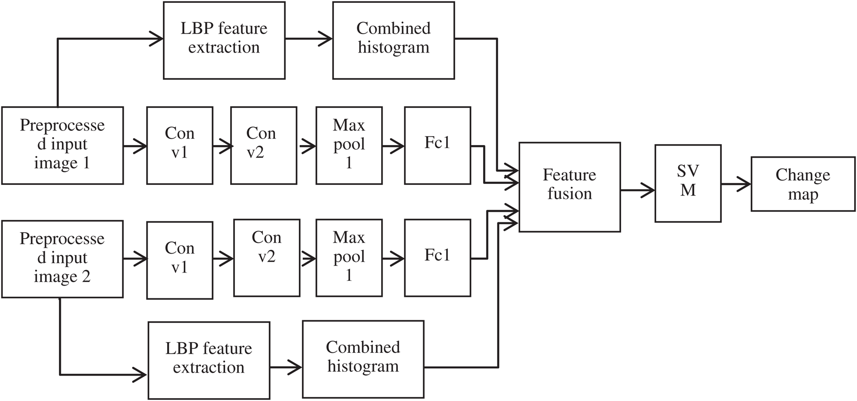
Figure 1: Framework of the proposed method

Here we take into consideration two images as input. Image registration process is not necessary owing to the fact that the two images are from the same sensor and capture bitemporal images of the same area. The proposed method contains four main stages namely: Image preprocessing, Feature extraction, Fusion and Classification. The input of the two-channel CNN is a patch of size 5 × 5 represented by p1,i and p2,i where i = 1, 2,….N taken from each source image and are fed individually into CNN modules where spatio-spectral features are extracted. N denotes the number of pixels in the image. Patch from the image is considered as input since it takes into account both spectral and spatial details. The textural information is extracted from the source images using Local Binary Pattern. In the second stage, the textural and spatio-spectral features extracted from each source image are fused by concatenation. In the final stage, the change map is obtained after classification of the change and no-change areas.

The network comprises of two convolutional layers and one max-pooling layer. Each convolutional layer has a kernel size of 2 × 2 and each max-pooling layer has a kernel size of 2 × 2. The output of the fully connected layer in each channel are concatenated with the textural features in both channels. The fused output is classified using SVM to generate a binary output in the form of a change map.

2.2 CNN Based Model-Motivation and Advantages

The generation of change map is a binary classification problem. Here fusion process can be viewed similar to a classifier and hence it is suitable to use CNN for feature fusion of bitemporal images. The CNN model contains a feature extraction module which comprises of alternately arranged convolutional and max-pooling layers and a classifier module. Traditionally fusion is performed using transformation techniques such as Discrete Wavelet Transforms (DWT). DWT method can be said to be based on filtering procedure [31]. The main operation involved in CNN is convolution, it is practically possible to use CNN for fusion.

The fusion process generally involves designing complex models and rules. This is taken care of by a trained CNN. Designing of the CNN architecture is also made easier with the development of deep learning platforms such as Caffe, MaxConvNet etc.

2.3 Image Preprocessing

Image preprocessing method is carried out to reduce any disparities between the bi-temporal source images that may arise due to the variations in atmospheric conditions at the time of image acquisition [32,33]. Since the images are acquired by the same sensor, image registration is not necessary. The success of the change detection technique is decided by the quality of the images used. To address this, a traditional bilateral filter is used for enhancing the source images. The choice of bilateral filter is obvious since it is an edge preserving filter which can denoise the image and also guarantees that all the edge information resembles that in source images [34]. This is of utmost importance especially due to the use of image fusion for change detection.

The bilateral filter output can be evaluated using Eq. (1) as [35]:

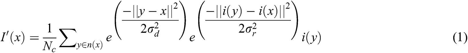
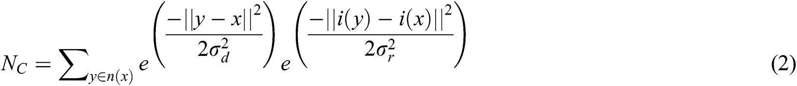
where x and y are the pixel co-ordinates, n(x) is the spatial neighborhood of i(x), σd and σr are the spatial and intensity domain controlling parameters. Nc is the normalization factor which can be computed using Eq. (2) as:

With the aim of preserving the edge information in the image and removing the noise, the bilateral filter can be considered as the most reliable preprocessing filter [36]. Fig. 2 shows the pre-processing output for a sample image.

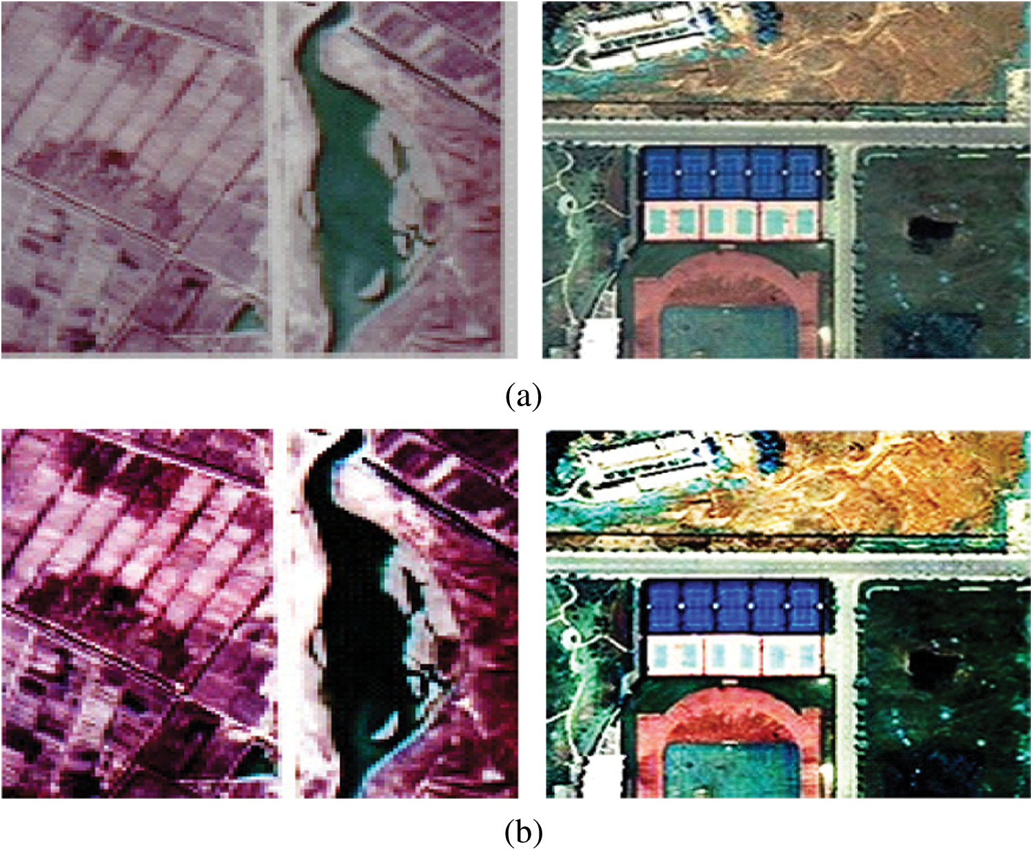
Figure 2: Preprocessing output (a) input image (b) enhanced image

Source images are low resolution images but contain rich spatial and textural information. To extract even the slightest of features, it is essential that the source image be enhanced for effective change classification. A low resolution image if used directly for classification can result in poor classification accuracy resulting from misclassified pixels due to the ineffectiveness in identifying features due to noise. Bilateral filter being a denoising as well as edge preserving filter can solve this issue to remove the noise components and enhance the edge details.

2.4 Spatio-Spectral Feature Extraction Using CNN

Spatio-spectral features are of great significance in detecting changes. The traditionally used algorithms such as algebra-based and transformation based change detection methods fail to capture the application specific features accurately. There are various neural network models such as Multilayer Perceptron model which can extract these features. Though it seems to be an interesting option, it suffers from the drawback that it has a large number of learnable parameters. This is of great concern since the training samples for change detection related applications are very less. Also such models treat the multispectral samples as vectors and ignore the 2D properties of the remote sensing images [37].

CNN is a deep learning algorithm which is useful for object recognition and its classification. CNN is a very good option for feature extraction since it is capable of automatically detecting 2D spatial and spectral features in multispectral remote sensing images. In addition, it is simpler to use and is very generic. Generally, a CNN comprises of alternately arranged convolutional and pooling layers to form a deep architectural model. 1D CNN is a commonly used algorithm in anomaly detection and biomedical data classification but it ignores the spatial features in the data. We utilize the 2D convolution operation on feature maps obtained from different bands in the multispectral image [38].

1) Convolutional Layer: The convolutional layer used in the paper can be defined using Eq. (3) as

where g is the input feature map, w and b represent the convolution kernel and the bias respectively. * is the convolution operator, k is the kth layer of the network, h is the output feature map of the convolutional layer. One can increase the dimension of the neighborhoods for better accuracy at the cost of increased time to train the network. Here the convolutional layer uses 3 × 3 filters to extract the spatio-spectral features.

2) Pooling Layer: For images of large size, it is desired to reduce the number of trainable parameters. For this purpose, we add pooling layers between the convolutional layers. The main aim of the pooling layer is to reduce the complexity by minimizing the spatial size of the image. The pooling layer can be defined using Eq. (4) as

where f is type of pooling operation with max being the max-pooling function used here and h is the output of the pooling layer. Max pooling is a down sampling method in CNN. In this work we have considered the stride as 2 and the max operation is done on each depth dimension of the convolution layer output.

3) Fully Connected Layer: Fully connected layer is a Multi-Layer Perceptron model which can obtain deep features which will help in classification. The fully connected layer is modeled using Eq. (5) as

where hl is the input of the fully connected layer l, and wl and bl are the weights and bias, respectively and yl is the output.

Visualization of the feature maps in different convolutional layers is given in Fig. 3.

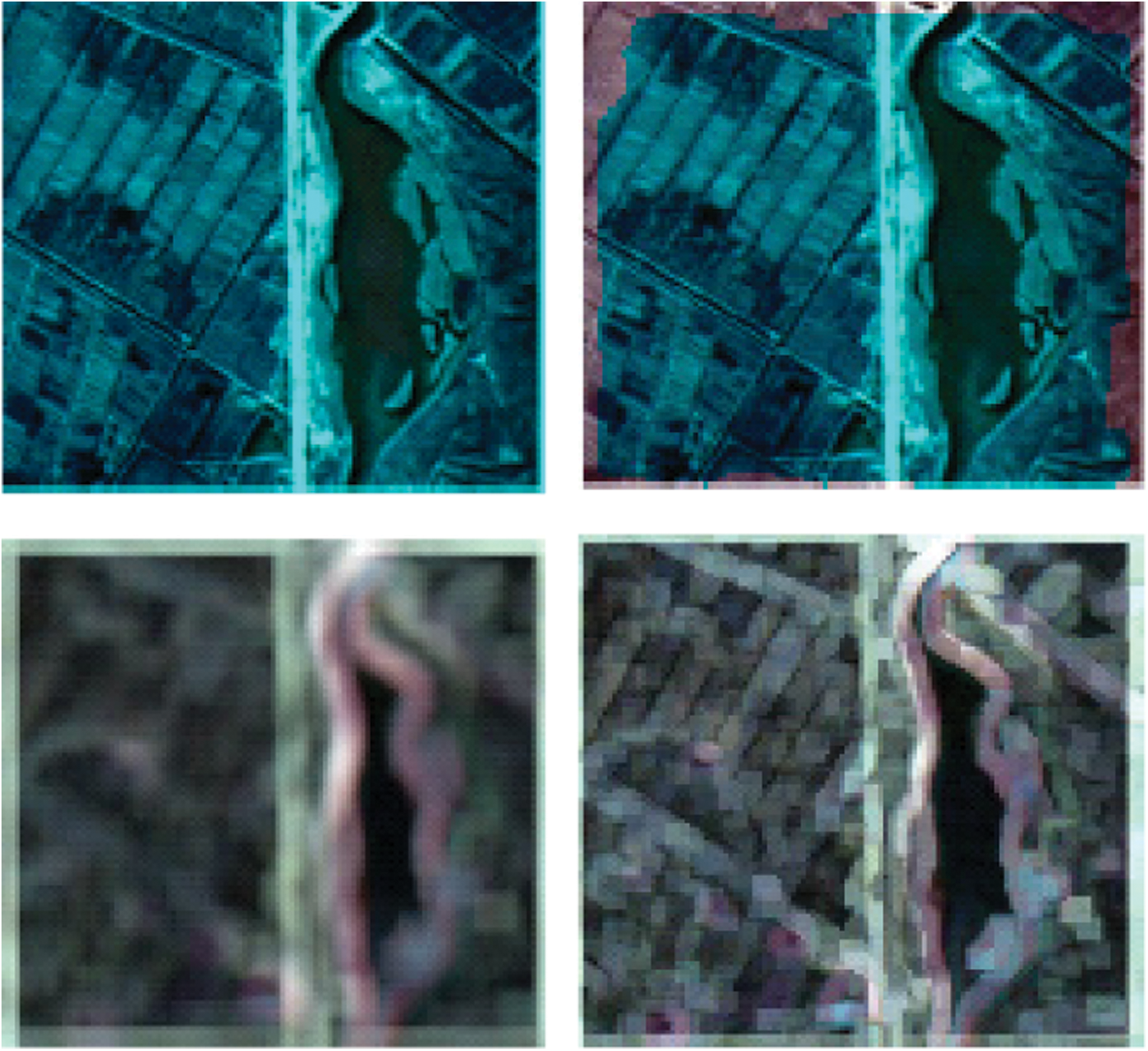
Figure 3: Feature map for within different convolutional layers

A convolutional layer condenses the input by extracting features of interest from it and produces feature maps in response. This feature map is propagated forward to reach the max-pooling layer (prior to the fully-connected layers), and extract the activations at that layer. The output of the max-pooling layer which is flattened and fed into the fully connected layers. Hence we obtain feature vector at the output of the fully connected layer. The initial convolution layer extracts features pertaining to the details in the satellite image. These features have close resemblance to the original image. The next convolution layer extracts contours, shape and related features.

2.5 Textural Feature Extraction Using LBP

Texture defines the local spatial structure and contrast in an image. Most of the methods for textural analysis are based on the gray levels in the image. Here LBP is used to extract the textural information in the image. By taking the central pixel Cp, the neighboring pixels are assigned binary codes 0 or 1 based on whether the neighboring values are greater or lesser than the central pixel. By considering a circular neighborhood with radius 1, the LBP code for the center pixel (x,y) is computed using Eqs. (6) and (7) as:

where

where C = k−1 is the number of sampling points on the circle with radius r. Cc is the central pixel and Cn is the neighboring pixel. Fig. 4 shows the LBP binary thresholding procedure.

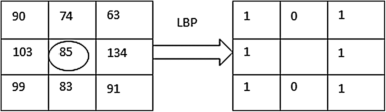
Figure 4: LBP binary thresholding

Once the LBP labels are obtained, the histogram is computed over each local patch. Similarly LBP operator is applied over all the patches and the histograms are concatenated to form a feature vector. LBP feature map and the equivalent histogram are given in Fig. 5.

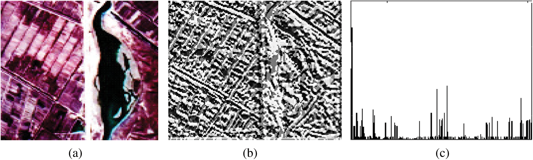
Figure 5: (a) Source image (b) LBP feature image (c) LBP histogram

2.6 Feature Fusion and Its Significance

Feature fusion helps in learning image features fully for describing their rich internal information. It plays a significant role in data fusion. The importance of feature fusion lies in the fact that different feature vectors from the same image reflect different characteristics of the image and by combining them, the effective discriminatory information is retained and the redundant information is eliminated to a great extend. Hence feature fusion has the capability to derive and gain the most effective and least dimensional feature vector sets that benefit the final outcome. To get more comprehensive feature representation of satellite image, the high level features extracted using CNN network and the textural features extracted using LBP are fused. Low level features extracted using the convolution layer in CNN are supplemented with the edge and textural features to reinforce the feature representation. Feature concatenation is used for feature fusion. LBP features represent the local texture information in the image while CNN extracts spatial and spectral features in each stage to form high level features. The deep features from the two channels are denoted as cnn1 and cnn2 respectively. Similarly, the textural feature vector from the two channels are named as tex1 and tex2. The features in each branch are concatenated as (tex1, cnn1, tex2, cnn2) into a single feature vector.. Before stacking of the feature sets is done, feature normalization is done using linear transformation. It converts the feature values in the range [0,1]. A diagrammatic representation of the feature fusion is depicted in Fig. 6.

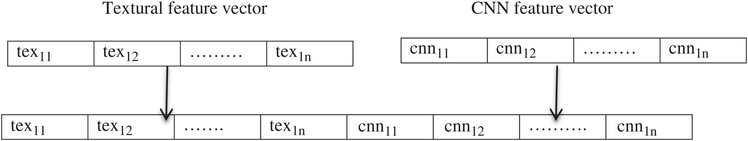
Figure 6: Feature fusion

After feature extraction, in the last fully connected layer the CNN and texture features are concatenated into a composite vector with weight 1:1 and fed into SVM for classification.

2.7 Classification and Change Map Generation

SVM is mainly used for binary classification problem. Features extracted and concatenated are classified using SVM. Let the training data and the corresponding labels be represented as (xn, yn) where n = 1, 2…N and yn ε{-1, 1}. Binary classes are separated using an optical hyper plane as shown in Eqs. (8) and (9) as:

with

where ϕ represents the non-linear kernel mapping which maps the input x to m dimensional space, n denotes the sample number, p represents the bias, regularization parameter is ζ and ω denotes the weight.

Radial Basis Function is used here and is given using Eq. (10) as:

where width is σ and the decision function is given using Eq. (11):

Once the classifier is applied on the fusion output, a binary change map is generated where white and black regions represent the changed and unchanged regions. It is revealed from the change map where the changes have occurred and whether the region has changed. It is using these change maps that land change decisions can be made.

3  Experimental Results and Discussion

3.1 Datasets

The dataset used for the work are acquired from GF-1 satellite and SPOT-5 satellite. The dataset comprises of sets of bitemporal satellite images of size 512 × 512. The first sample is taken from Chongquing region in China which shows building changes and captured during 2004 and 2008. The second dataset is from Hongqi canal region showing the changes in Hongqi riverway and are captured during 2013 and 2015. All sets are provided with their corresponding ground truth imagery. The images have a spatial resolution of 2 m. The work is implemented in MATLAB 2018a. The CNN architecture is carried out using Caffe deep learning library [39] on a system (i7-6800k CPU, 16 GB RAM). Fig. 7 shows a sample change detection image set along with the ground truth. The datasets are orthorectified and co-registered. But if multi-sensor images are considered, then the images need to be registered.

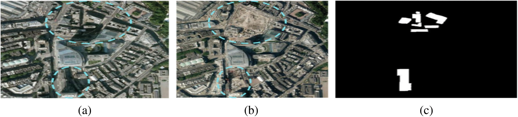
Figure 7: (a, b) Sample change detection images c. Ground truth

To analyze the performance of the proposed CNN based feature fusion, various existing change detection techniques such as MRF, CVA, SCCN and SCNN + SVM are compared.

3.2 Parameter Settings

The parameters set for the CNN architecture such as the kernel size and stride in each layer are shown in Tab. 1.

Table 1: CNN architecture setting

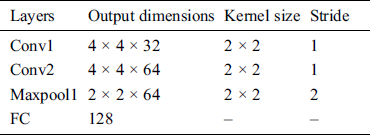
The network is trained based on the Caffe framework. All the parameters of this framework are fixed as follows: Bias b = 0 and a schedule decay of 0.04 with a small learning rate of 1e-04. The training on the network is done for 50 epochs. In the training phase, an equal number of changed and unchanged pairwise samples are used. Then, these samples are fed into the network to extract the features. Finally, the extracted features and the target labels are applied to train the SVM. Remaining samples are used for testing.

3.3 Performance Analysis

Here the aim is to compare the performance of the proposed CNN based feature fusion with other traditional change detection techniques. The change detection algorithms are applied on all the three dataset and the results for all the change detection methods (MRF, CVA, SCCN and SCNN+SVM) are shown. Objectively evaluating change detection is very important to examine the change detection accuracy. The performance of the change detection algorithm has been evaluated by calculating metrics such as kappa coefficient and overall accuracy. Overall accuracy gives a measure of the number of image pixels which are classified correctly to the total input samples. Kappa coefficient is a performance metric for change detection. It is calculated using Eq. (12) as

where k1 is the classification accuracy or the actual agreement and k2 is the expected agreement in each class. F_Measure score is another measure of accuracy and is found using Eq. (13) as:

Here Fp and Fr are computed using Eqs. (14) and (15) as:

Fp and Fr are also called precision and recall respectively. F_Measure lies between 0 and 1. A high precision and recall value guarantees that the change detection algorithm used is good.

3.4 Results

The first sample is taken from Chongquing region in China and the second sample is taken from Hongqi canal region. The change maps of the proposed method and the traditional methods are shown in Figs. 8 and 9. Figs. 8a–8c and 9a–9c show the source images with the ground truth where the black and white areas indicate the no change and change areas, respectively.

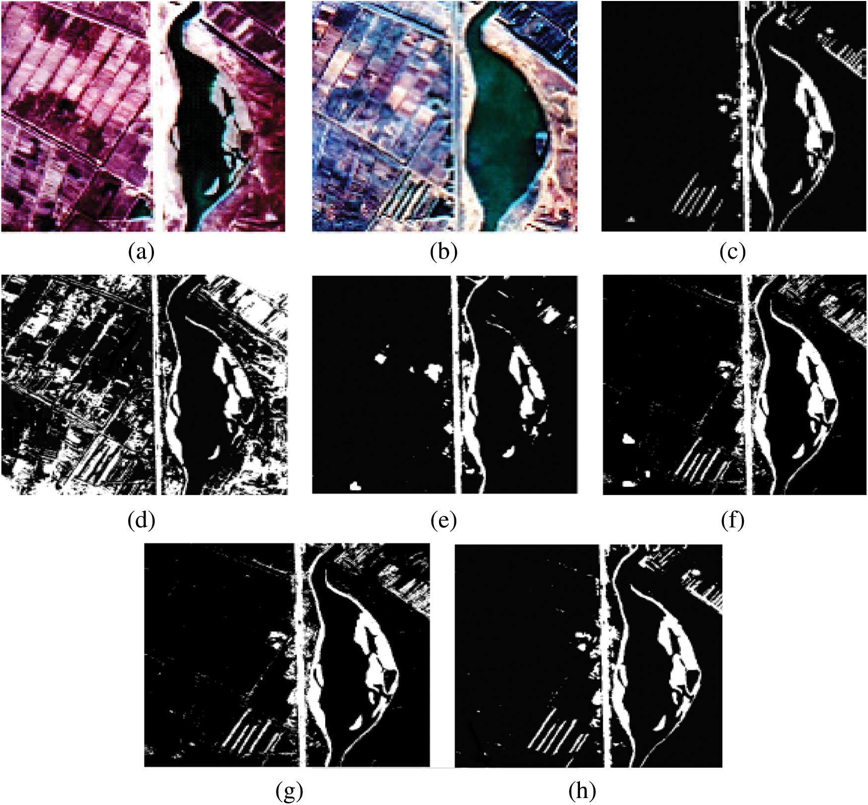
Figure 8: Dataset 1 (a, b) input images c. Ground truth d. CVA e. MRF f. SCCN g. SCNN+SVM h. Proposed method

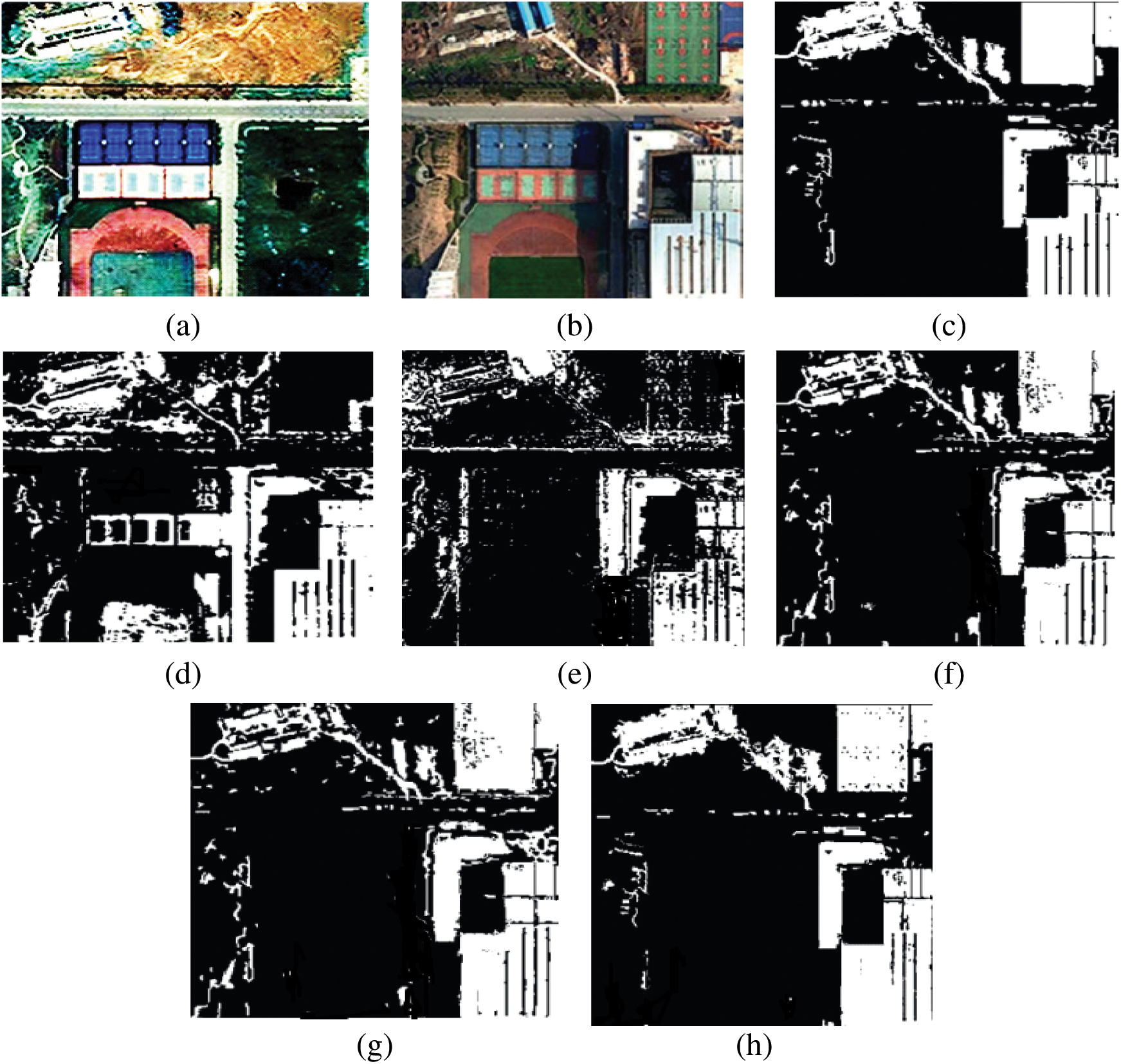
Figure 9: Dataset 2 (a, b) input images c. Ground truth d. CVA e. MRF f. SCCN g. SCNN+SVM h. Proposed method

CVA and MRF based change detection gives poor result on this dataset as shown in Figs. 8d, 8e, 9d and 9e. In CVA, the main reason for its poor performance is attributed to the fact that the number of unchanged pixels classified as changed ones is high. But in MRF, changed pixels are misclassified as unchanged pixels. CVA and MRF are both unsupervised change detection method which utilize manual features obtained using prior information and data. SCCN, SCNN + SVM and proposed method can detect the changes better than CVA and MRF due to the presence of deep learning to extract deep features. SCNN is an unsupervised method while SCNN + SVM and the proposed method are supervised. SCCN can detect the changes better but there are some noises generated in the binary map. With the use of SVM, the classification result has improved and the change maps shown in Figs. 8g and 9g are better over SCCN. The proposed method is seen to perform better as seen in Figs. 8h and 9h since there is decrease in the noisy areas in the image and can reduce the false positives from change areas. The number of isolated pixels along the canal and the building regions have decreased to a large amount when compared to the other methods. The fusion of spatial, spectral and textural features in the proposed method are effective in finding the change areas better when compared to other methods.

The quantitative performance is analyzed by computing accuracy (OA), kappa coefficient and F_measure (F1). Tab. 2 gives the change detection performance metrics (Overall accuracy, Kappa Coefficient, F_measure) for the two datasets.

Table 2: Change detection performance metrics for database

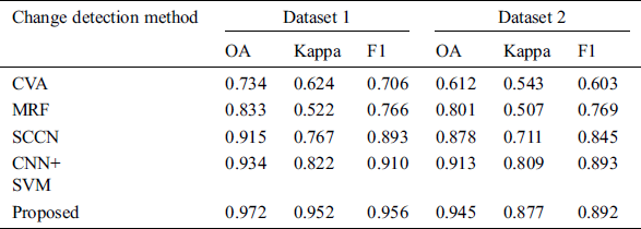
It can be observed from the table that the proposed method gives better results in terms of OA, kappa value and F_measure compared to other methods. The proposed method uses fusion of different features which can better represent the image changes and hence performs better quantitatively and qualitatively.

An ROC curve is a useful technique for visualizing, organizing and selecting classifiers based on their performance and is often adopted as a plot reflective of the classifier’s performance. The Receiver Operating Characteristic (ROC) is a measure of a classifier’s predictive quality that compares and visualizes the tradeoff between the model’s sensitivity and specificity. The value for the ROC plot is the area under the ROC curve in which a high value indicates that the algorithm used is good. A perfect classifier is visualized as one which yields a point in in the upper left corner or coordinate (0,1) of the ROC space, representing 100% sensitivity (no false negatives) and 100% specificity (no false positives). Fig. 10 gives the ROC plot for the two datasets for the different change detection techniques. From the graph, it is clear that the proposed the proposed method is better over traditional techniques for the two datasets.

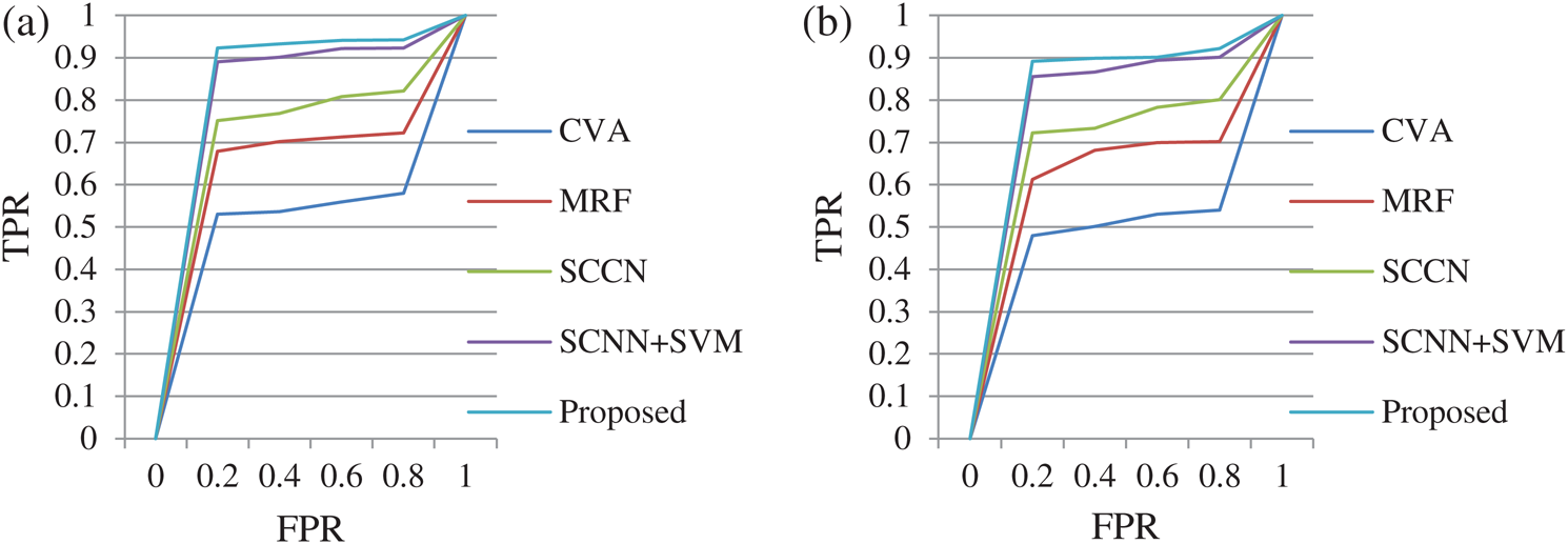
Figure 10: ROC plot for the different change detection methods for (a) Dataset 1 (b) Dataset 2

A good change detection algorithm will have its ROC plot nearer to the top-left corner in the co-ordinate system. The numerical value for the ROC plot is obtained from the area under the ROC curve or the AUC. High AUC value indicates that the change detection algorithm used is good and can distinguish between change and unchanged areas effectively. From Fig. 7, it is clear that the proposed technique outperforms the traditional change detection techniques for the two datasets by viewing the closeness of the curve to the top left corner of the plot.

4  Conclusion

This work describes a CNN based multi-feature fusion for bi-temporal image classification. A two-channel CNN framework is designed to perform feature extraction. CNN extracts the deep spatio-spectral features from the individual channels in bitemporal source images. The textural information is extracted using LBP method. Features are concatenated and classified to get binary change map. The extraction of the deep features in the remote sensing images makes the proposed method a feasible and attractive solution for change detection. The change detection output shows the attractiveness of CNN based fusion model which gave a better accuracy in comparison to conventional change detection methods. Future work can be extended to improve the bi-temporal change classification accuracy by modifying the fusion rule, classification algorithm and increasing the layers in the neural network model.

Funding Statement: The authors received no specific funding for this study.

Conflicts of Interest: The authors declare that they have no conflicts of interest to report regarding the present study.

References

This work is licensed under a Creative Commons Attribution 4.0 International License, which permits unrestricted use, distribution, and reproduction in any medium, provided the original work is properly cited.

References

1A. L. Choodarathnakara, T. A. Kumar and S. Koliwad. (2012), “Mixed pixels: A challenge in remote sensing data classification for improving performance. ,” International Journal of Advanced Research in Computer Engineering and Technology, vol. 1, pp, 2278–1323, .
2G. Cao, X. Li and L. Zhou. (2016), “Unsupervised change detection in high spatial resolution remote sensing images based on a conditional random field model. ,” European Journal of Remote Sensing, vol. 49, no. (1), pp, 225–237, . [Google Scholar]
3H. Zhuang, K. Deng, H. Fan and M. Yu. (2016), “Strategies combining spectral angle mapper and change vector analysis to unsupervised change detection in multispectral images. ,” IEEE Geoscience and Remote Sensing Letters, vol. 13, no. (5), pp, 681–685, . [Google Scholar]
4J. S. Deng, K. Wang, Y. H. Deng and G. J. Qi. (2008), “PCA-based land-use change detection and analysis using multitemporal and multisensor satellite data. ,” International Journal of Remote Sensing, vol. 29, no. (16), pp, 4823–4838, . [Google Scholar]
5A. Tahraoui, R. Kheddam, A. Bouakache and A. Belhadj-Aissa. (2018), “Land change detection using multivariate alteration detection and chi squared test thresholding. ,” in Proc. of ATSIP, Sousse, Tunisia, pp, 1–6, . [Google Scholar]
6N. Venugopal. (2019), “Sample selection based change detection with dilated network learning in remote sensing images. ,” Sensing and Imaging, vol. 20, no. (31), pp, 1–22, . [Google Scholar]
7S. Saha, F. Bovolo and L. Bruzzone. (2019), “Unsupervised deep change vector analysis for multiple-change detection in VHR images. ,” IEEE Transactions on Geoscience and Remote Sensing, vol. 57, no. (6), pp, 3677–3693, . [Google Scholar]
8H. Zhang, Y. Li, Y. Zhang and Q. Shen. (2017), “Spectral-spatial classification of hyperspectral imagery using a dual-channel convolutional neural network. ,” Remote Sensing Letters, vol. 8, no. (5), pp, 438–447, . [Google Scholar]
9F. Gao, J. Dong, B. Li and Q. Xu. (2016), “Automatic change detection in synthetic aperture radar images based on PCANet. ,” IEEE Geoscience and Remote Sensing Letters, vol. 13, no. (12), pp, 1792–1796, . [Google Scholar]
10N. Lv, C. Chen, T. Qiu and A. K. Sangaiah. (2018), “Deep learning and superpixel feature extraction based on contractive autoencoder for change detection in SAR images. ,” IEEE Transactions on Industrial Informatics, vol. 14, no. (12), pp, 5530–5538, . [Google Scholar]
11H. Lyu, H. Lu and L. Mou. (2016), “Learning a transferable change rule from a recurrent neural network for land cover change detection. ,” Remote Sensing, vol. 8, no. (6), pp, 1–22, . [Google Scholar]
12S. Ghosh, M. Roy and A. Ghosh. (2014), “Semi-supervised change detection using modified self-organizing feature map neural network. ,” Applied Soft Computing, vol. 15, pp, 1–20, . [Google Scholar]
13J. Liu, M. Gong, K. Qin and P. Zhang. (2018), “A deep convolutional coupling network for change detection based on heterogeneous optical and radar images. ,” IEEE Transactions on Neural Networks and Learning Systems, vol. 29, no. (3), pp, 545–559, . [Google Scholar]
14J. Zhang, X. Jin, J. Sun, J. Wang and A. K. Sangaiah. (2020), “Spatial and semantic convolutional features for robust visual object tracking. ,” Multimedia Tools and Applications, vol. 79, no. (21–22), pp, 15095–15115, . [Google Scholar]
15W. Wang, Y. T. Li, T. Zou, X. Wang, J. You et al. (2020). , “A novel image classification approach via Dense-MobileNet models, Mobile Information Systems. ,” Mobile Information Systems, vol. 2020, pp, 1–8, . [Google Scholar]
16Y. Chen, J. Tao, L. Liu, J. Xiong, R. Xia et al. (2020). , “Research of improving semantic image segmentation based on a feature fusion model. ,” Journal of Ambient Intelligence and Humanized Computing, vol. 29, no. (2), pp, 1–13, . [Google Scholar]
17S. Zhou and B. Tan. (2020), “Electrocardiogram soft computing using hybrid deep learning CNN-ELM. ,” Applied Soft Computing, vol. 86, pp, 1–11, . [Google Scholar]
18S. Pan, H. Guan, Y. Chen, Y. Yu, W. Nunes Gonçalves et al. (2020). , “Land-cover classification of multispectral LiDAR data using CNN with optimized hyper-parameters, ISPRS. ,” Journal of Photogrammetry and Remote Sensing, vol. 166, pp, 241–254, . [Google Scholar]
19H. Hermessi, O. Mourali and E. Zagrouba. (2018), “Convolutional neural network-based multimodal image fusion via similarity learning in the shearlet domain. ,” Neural Computing and Applications, vol. 30, no. (7), pp, 2029–2045, . [Google Scholar]
20M. Amin-Naji, A. Aghagolzadeh and M. Ezoji. (2019), “Ensemble of CNN for multi-focus image fusion. ,” Information Fusion, vol. 51, pp, 201–214, . [Google Scholar]
21X. Luo, Z. Zhang and X. Wu. (2016), “A novel algorithm of remote sensing image fusion based on shift-invariant Shearlet transform and regional selection. ,” AEU-International Journal of Electronics and Communications, vol. 70, no. (2), pp, 186–197, . [Google Scholar]
22D. Anandhi and S. Valli. (2018), “An algorithm for multi-sensor image fusion using maximum a posteriori and nonsubsampled contourlet transform. ,” Computers & Electrical Engineering, vol. 65, pp, 139–152, . [Google Scholar]
23Z. Zhu, H. Yin, Y. Chai, Y. Li and G. Qi. (2018), “A novel multi-modality image fusion method based on image decomposition and sparse representation. ,” Information Sciences, vol. 432, pp, 516–529, . [Google Scholar]
24Y. Zhang, L. Zhang, X. Bai and L. Zhang. (2017), “Infrared and visual image fusion through infrared feature extraction and visual information preservation. ,” Infrared Physics & Technology, vol. 83, pp, 227–237, . [Google Scholar]
25C. Du, S. Gao, Y. Liu and B. Gao. (2019), “Multi-focus image fusion using deep support value convolutional neural network. ,” Optik, vol. 176, pp, 567–578, . [Google Scholar]
26J. Li, Q. Hu and M. Ai. (2018), “Multispectral and panchromatic image fusion based on spatial consistency. ,” International Journal of Remote Sensing, vol. 39, no. (4), pp, 1017–1041, . [Google Scholar]
27H. Shen, M. Jiang, J. Li, Q. Yuan, Y. Wei et al. (2019). , “Spatial–spectral fusion by combining deep learning and variational model. ,” IEEE Transactions on Geoscience and Remote Sensing, vol. 57, no. (8), pp, 6169–6181, . [Google Scholar]
28E. Vargas, H. Arguello and J. Y. Tourneret. (2019), “Spectral image fusion from compressive measurements using spectral unmixing and a sparse representation of abundance maps. ,” IEEE Transactions on Geoscience and Remote Sensing, vol. 57, no. (7), pp, 5043–5053, . [Google Scholar]
29Y. Chen, J. Wang, S. Liu, X. Chen, J. Xiong et al. (2019). , “Multiscale fast correlation filtering tracking algorithm based on a feature fusion model. ,” Concurrency and Computation: Practice and Experience, vol. 47, no. (5), pp, e5533, . [Google Scholar]
30C. Wang, G. Peng and B. De Baets. (2020), “Deep feature fusion through adaptive discriminative metric learning for scene recognition. ,” Information Fusion, vol. 63, pp, 1–12, . [Google Scholar]
31Y. Liu, X. Chen, H. Peng and Z. Wang. (2017), “Multi-focus image fusion with a deep convolutional neural network. ,” Information Fusion, vol. 36, pp, 191–207, . [Google Scholar]
32I. Fawwaz, M. Zarlis, Suherman and R. F. Rahmat. (2018), “The edge detection enhancement on satellite image using bilateral filter. ,” IOP Conference Series: Materials Science and Engineering, vol. 308, pp, 1–9, . [Google Scholar]
33S. Srisuk, T. N. Yad, A. Muang and N. Phanom. (2014), “Bilateral filtering as a tool for image smoothing with edge preserving properties. ,” in Proc. of Int. Electrical Engineering Cong., Chonburi, Thailand, pp, 1–4, . [Google Scholar]
34F. Hofheinz, J. Langner, B. Beuthien-Baumann, L. Oehme, J. Steinbach et al. (2011). , “Suitability of bilateral filtering for edge-preserving noise reduction in PET. ,” EJNMMI Research, vol. 1, no. (1), pp, 1–9, . [Google Scholar]
35V. Anoop and P. R. Bipin. (2019), “Medical image enhancement by a bilateral filter using optimization technique. ,” Journal of Medical Systems, vol. 43, no. (8), pp, 1–12, . [Google Scholar]
36Q. Yang, S. Wang and N. Ahuja. (2010), “Real-time specular highlight removal using bilateral filtering. ,” in European Conf. on Computer Vision, Crete, Greece, pp, 87–100, . [Google Scholar]
37L. Mou, L. Bruzzone and X. X. Zhu. (2019), “Learning spectral-spatialoral features via a recurrent convolutional neural network for change detection in multispectral imagery. ,” IEEE Transactions on Geoscience and Remote Sensing, vol. 57, no. (2), pp, 924–935, . [Google Scholar]
38B. Liu, X. Yu, P. Zhang, A. Yu, Q. Fu et al. (2018). , “Supervised deep feature extraction for hyperspectral image classification. ,” IEEE Transactions on Geoscience and Remote Sensing, vol. 56, no. (4), pp, 1909–1921, . [Google Scholar]
39Y. Jia, E. Shelhamer, J. Donahue, S. Karayev, J. Long et al. (2014). , “Convolutional architecture for fast feature embedding. ,” in Proc. of ACM Conf. on Multimedia, Florida, USA, pp, 675–678, . [Google Scholar]