DOI:10.32604/cmc.2020.012948
| Computers, Materials & Continua DOI:10.32604/cmc.2020.012948 | |
| Article |
Three-Dimensional Meshfree Analysis of Interlocking Concrete Blocks for Step Seawall Structure
1Soete Laboratory, Faculty of Engineering and Architecture, Ghent University, Technologiepark Zwijnaarde 903, B-9052, Zwijnaarde, Belgium
2University of Science and Technology, The University of Danang, Da Nang City, Vietnam
3CIRTech Institute, Ho Chi Minh City University of Technology, Ho Chi Minh City, Vietnam
4Division of Computational Mechanics, Ton Duc Thang University, Ho Chi Minh City, Vietnam
5Faculty of Civil Engineering, Ton Duc Thang University, Ho Chi Minh City, Vietnam
*Corresponding Author: Magd Abdel-Wahab. Email: magd.abdelwahab@tdtu.edu.vn
Received: 19 July 2020; Accepted: 21 August 2020
Abstract: This study adapts the flexible characteristic of meshfree method in analyzing three-dimensional (3D) complex geometry structures, which are the interlocking concrete blocks of step seawall. The elastostatic behavior of the block is analysed by solving the Galerkin weak form formulation over local support domain. The 3D moving least square (MLS) approximation is applied to build the interpolation functions of unknowns. The pre-defined number of nodes in an integration domain ranging from 10 to 60 nodes is also investigated for their effect on the studied results. The accuracy and efficiency of the studied method on 3D elastostatic responses are validated through the comparison with the solutions of standard finite element method (FEM) using linear shape functions on tetrahedral elements and the well-known commercial software, ANSYS. The results show that elastostatic responses of studied concrete block obtained by meshfree method converge faster and are more accurate than those of standard FEM. The studied meshfree method is effective in the analysis of static responses of complex geometry structures. The amount of discretised nodes within the integration domain used in building MLS shape functions should be in the range from 30 to 60 nodes and should not be less than 20 nodes.
Keywords: Meshfree method; local support domain; moving least square shape function; 3D elastostatic behavior; complex geometry
Meshfree methods, that have been developed recent years, are believed to show more advantages than finite element method in dealing with problems of fluid flows, large deformations, crack growth along the complex path, fragment-impact, complex shape structures and so on [1–5]. By using meshfree method, the prediction of unknowns is performed with the aid of discretized nodes only. There are many different meshfree approaches, which have achieved remarkable solutions for numerical problems, such as smoothed particle hydrodynamics (SPH) method [6–10], finite difference methods with scattered points [11], element free Galerkin (EFG) method [8–12], meshless local Petrov-Galerkin method [13,14], dual-horizon peridynamics [15], nonlocal operator method [16], meshfree radial point interpolation method (RPIM) [17,18], natural neighbour radial point interpolation method (NNRPIM) [19], etc.
Meshfree methods have been implemented in various fields and problems of engineering, in which problems of liquid and/or interaction between solid and liquid are solved by using SPH method. Ren et al. [20] and Akbari et al. [21] analysed the 2D interaction model of wave action through pervious breakwater by developing an improved SPH method. The method was also used in the analysis of nano flows [22], multiphase flows [23] and so on. The EFG method was applied to problems of 2D solid mechanics and heat transmission [24,25]. The analysis of boundary value problems by using meshfree method with high order approximation was reported by Milewski [26]. In addition, applications of meshless methods on three-dimensional solid mechanics problems were also presented. The 3D problems with singularity and heterogeneous material were solved by using MLPG method [27]. The radial point interpolation method was applied to obtained 3D elasticity responses of an axletree base [28]. An improvement of radial point interpolation method by combining with natural neighbour finite element method was reported and successfully applied for a simple case of three-dimensional solid [19].
EFG is one of the most known and robust meshfree methods. It is a development of Galerkin method applied on partial differential equations. EFG analyses the weak form formulations of displacement field similarly to standard FEM. Nevertheless, a number of discretised nodes within structure domain are used for building approximation functions instead of FEM elements. Compared to traditional FEM, EFG method has many advantages. Firstly, the problem of meshing structure can be eliminated. Secondly, EFGM performance does not depend on nodal distribution. Additionally, EFGM does not require any special treatment for structure with incompressible material [25]. Therefore, the applications of EFGM and its improvement in the wide range of engineering problems have attracted the attention of many researchers such as the nonlinear analysis of Darcy-Forchheimer problems [12], heat transition problems [29,30], nonlinear calculation of solid structures [8–31], wave propagations of fluid analysis [32,33], etc. In this study, the implementation of EFGM in three-dimensional elastostatic analysis on complex geometry structure will be investigated. The detail of EFGM will be further discussed in the next section.
The process of forming shape functions is the main feature indicating the discrepancy between traditional finite element methods and meshless methods. Many meshfree shape functions have been successfully developed, which include moving least squares approximation, point interpolation, partition of unity (PU) and HP-clouds approximation [34]. Whereas, the MLS approximation is widely applied method with simplicity and reasonable accuracy [35]. The MLS shape functions are formulated based on a number of nodes within an integration domain instead of pre-defined element as in FEM. Unlike regular FEM mesh, in which the elements should not overlap with each other, the nodes connectivity in meshfree methods defines a structure through overlapping of support domains. The shape and size of these domains are crucial in stability and accuracy results obtained by using EFGM with MLS approximation. Liu et al. [28] reported in their particular study using radial point interpolation that the spherical support domain with pre-defined number of nodes ranging from 20 to 70 provided more stable results compared to the model with pre-defined support size (diameter). Extendedly, the former model will be studied for its effectiveness on results obtained by using MLS shape functions.
The objective of this study is to present the application of EFGM using moving least square approximation in analyzing elastostatic responses of three-dimensional structure with complex geometry. Effect of spherical support domains with pre-defined number of nodes, which are used for building MLS approximation, on convergence and accuracy of results is also investigated. The number of nodes in each domain ranges from 10 to 60. Each step increases by 10 nodes. The efficiency of the EFG method is verified by comparing the elastostatic responses of a complex concrete block with the results determined by standard FEM and commercial software ANSYS. Whereas, standard FEM uses linear tetrahedral elements and ANSYS uses 10-node tetrahedral elements. All the coding in this study including EFGM and standard FEM are performed using MATLAB program.
2 Element Free Galerkin Method in Three Dimension
The EFG method is a typical meshless method solving the Galerkin weak form by only using a set of distributed points. The shape functions of EFG method are formulated relying on MLS approximation over a local support domain, which contents a group of nodes. The EFGM is one of the most extensively applied meshless methods in many boundary value problems of solid mechanics. There are three components used to construct the moving least square approximations, which include a weight function; a basis, which is linear polynomial in this study; and coefficients depending on position. The weight function does not vanish only in support domain of current integration node. Connectivity of discretized nodes in meshfree structure is defined by overlapping of the nodal support domains. In general, the support domains can be any geometric shape and size. However, in this study, the spherical domains are taken into considering for its numerical simplicity.
Even though EFG is a meshless method, a background mesh is needed for solving the integration of Galerkin weak form. The MLS constructing process in 3D is described in this section.
2.1 Moving Least Square Approximation
Let us consider a spherical domain  containing N nodes (Fig. 1). The governing displacement of nodes is described as u(x). At each node, the displacement parameter is ui corresponding to u(x) at that node.
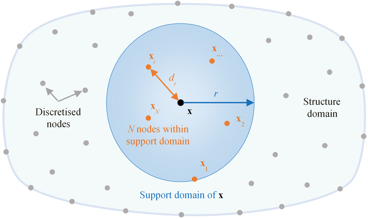
Figure 1: Support domain in building MLS approximation
The moving least square approximation uh(x) over domain  is given by:

where p(x) is the monomial basic function with the number of basis m:

In this study, 3D linear basic function is used as:

a(x) is a coefficient vector given as follows:

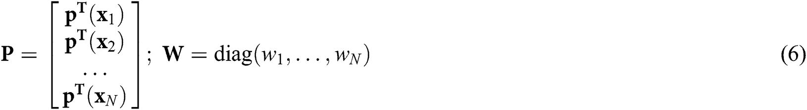
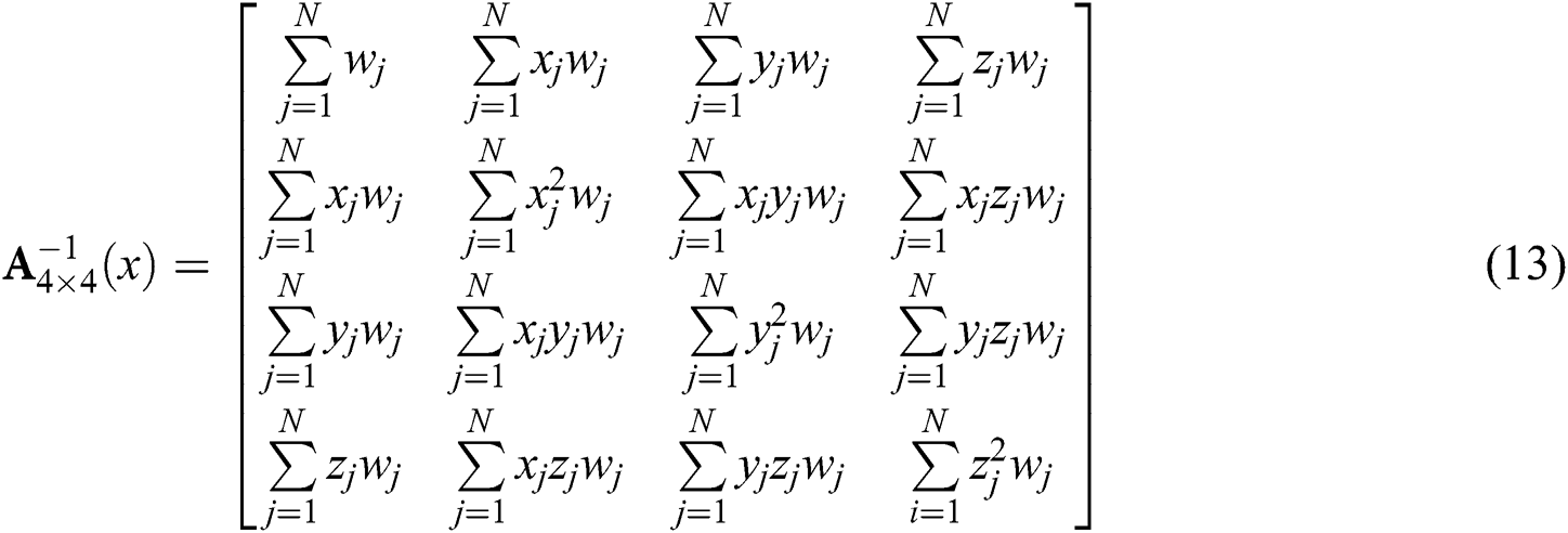
in which moment matrix A(x) is given by:

with wi is the weight function at node I within domain  and
and
and


Substituting Eqs. (3)–(8) to Eq. (1), the MLS approximation over domain  is given as:

where

In this work, a 4th order spline weight function is used as follows:
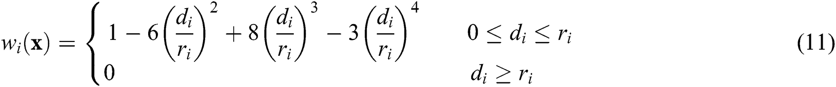
where di = |xi – x| is the distance between point xi and x, ri is the radius of the support of point xi for weight function.
2.2 Meshfree Analysis Procedure
The meshfree method is used to analyse three-dimensional solid structure using displacement based formulation. The codes are compiled in MATLAB program based on following steps:
Step 1
The domain of problem is discretised into arbitrarily distributing nodes:
•Numbering discretised nodes, creating background cells for integration, which are tetrahedral cells in this study.
•Assigning the physical properties of the analysed structure. The concrete material has Young’s modulus E of 30500 MPa and Poison’s ratio  of 0.2.
Step 2
The boundary value problem is presented through the differential equation with desired boundary conditions. For the fixed boundary, the displacements of corresponding DOFs of boundary are assigned as zeroes.
Step 3
Assembling global stiffness matrix constructed from weak form governing differential equation includes:
•Generating the Gauss points based on the background tetrahedral cells.
•Defining support domain for each Gauss point (looping over). A number of nodes in each support domain are pre-defined ranging from 10 to 60 nodes. In each step an increase of 10 nodes is applied for investigating the effect of support domain in the studied problems.
•Within the support domain, the derivatives of shape functions can be determined as in following formulations:
•The shapes functions of N nodes in the current domain are:

where
and
•The partial derivatives of the shape functions are calculated by re-writing Eq. (12) as [36]:

where

•Analysing the partial derivatives of C by following formulation:

with subscript, “,i” indicates the derivatives with respect to x, y or z.
•Hence, Eq. (15) can be determined as follows:

•After obtaining the partial derivatives of shape functions, the stiffness matrix is assembled similarly to standard finite element method.
•The assembling process of surface load matrix is similar to stiffness matrix, but the shape functions are used instead of their partial derivatives.
Step 4
The above discrete nodal equations of stiffness and force matrices are assembled into global matrices.
Step 5
The results of nodal displacements can be obtained by solving the standard discrete equations KU = F.
Step 6
The nodal stresses are determined by performing post-processing of the displacements obtained in Step 5.
The studied structure is a 3D concrete block of an interlocking step seawall (Fig. 2) [37]. In analysis using meshfree method, the number of discretised points in the support region is an important variable that greatly affects the accuracy, as well as, the convergence of the obtained solutions. Therefore, in this work, the number of nodes in the range from 10 to 60 is investigated with the increment step of 10 nodes. The recommended number of support domain nodes is, then, used for further analysing of elastostatic responses of the structure.
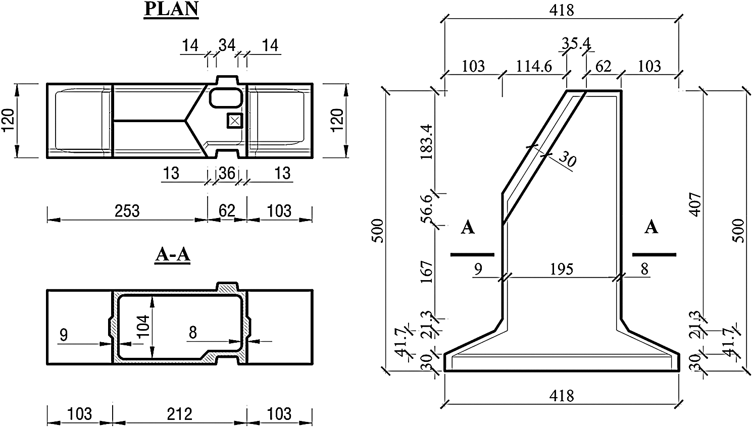
Figure 2: Sketch of studied concrete block
The displacement and stress responses are estimated by using EFG method in MATLAB program. The efficiency of EFG method is evaluated by making a comparison between the obtained solutions and those of standard FEM and ANSYS software. Fig. 3 illustrates the discretised models using EFG and standard FEM.
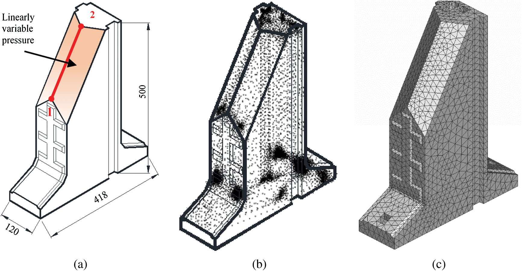
Figure 3: Three-dimensional models of the studied concrete block: a) the pressure is applied on block surfaces and edge 1–2 is used for extracting results, b) adaptively discretised nodes for EFG analysis and c) tetrahedral meshes for linear FEM analysis
The results shown in Figs. 4–6 are obtained by EFGM with various numbers of nodes in the support domain. Those figures show the convergent trends of elastostatic responses with the increase of global nodes. It is worth noting that “Reference” stands for results determined by ANSYS while the other legends represent the results obtained by meshfree method with corresponding nodal amount in support domains. In those figures, the existences of 10-node support domain responses are eliminated due to their lacking of accuracy. It is believed that with low number of support domain nodes, which is less than 20 in this study, the moment matrix A is close to singularity. Hence, it causes inaccurate results. With the same number of global points, when the number of nodes in interpolation domain increases, the accuracy of results increases accordingly. In addition, the support domain nodes higher than 30 can give more accurate results and faster convergence.
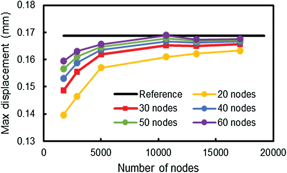
Figure 4: Convergence of maximum X-displacement for all cases of investigated support domains
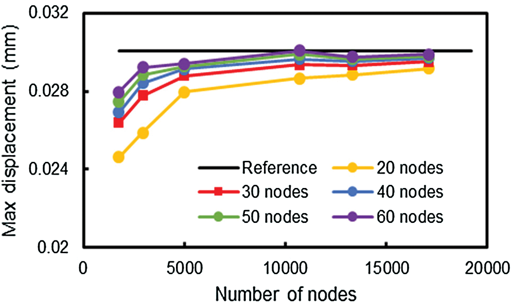
Figure 5: Convergence of maximum Z-displacement for all cases of investigated support domains
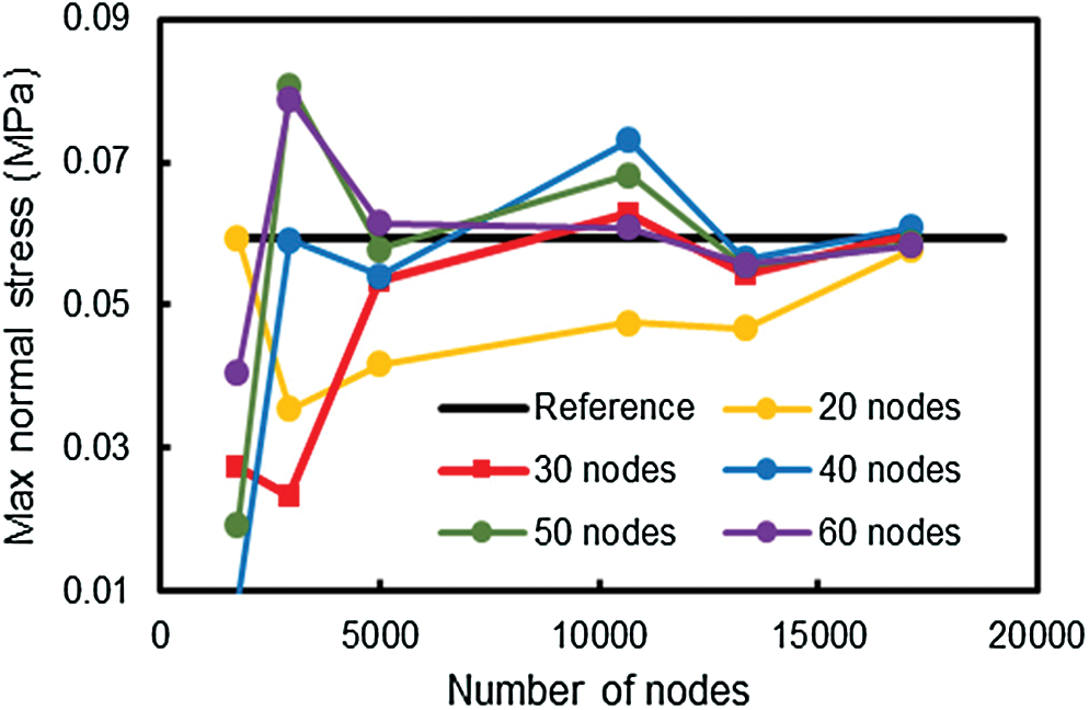
Figure 6: Convergence of maximum normal stress  for all cases of investigated support domains
Fig. 7 compares the computational time in hours of the meshfree method implementation with various number of nodes within the support domains. The 5000-discritized node block corresponding to the third mesh was investigated. The figure shows that the computational time increases gradually when the support nodes rise from 20 to 50 (no more than 6% compared to 20-node support domain). Nevertheless, when the support nodes reach 60, the computational time increases significantly (up to 26%).
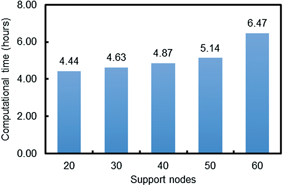
Figure 7: Computational time of the concrete block meshed into 5000 nodes with different support nodes
The following analysis uses 40-node domain for investigating elastostatic responses along edge 1–2 of the concrete block obtained by EFGM compared with FEM. The convergence studies of displacement and stress responses are performed and shown in Figs. 8–10. In these three figures, “Meshfree” represents the results determined by EFG method where “FEM” stands for the results obtained by standard FEM with linear tetrahedral elements. It can be observed that the solutions determined by EFGM converge much faster than those of FEM.
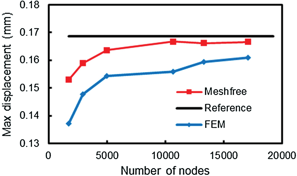
Figure 8: Convergence of maximum X-displacement obtained by EFG and FEM
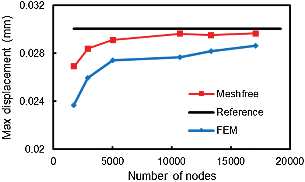
Figure 9: Convergence of maximum Z-displacement obtained by EFG and FEM
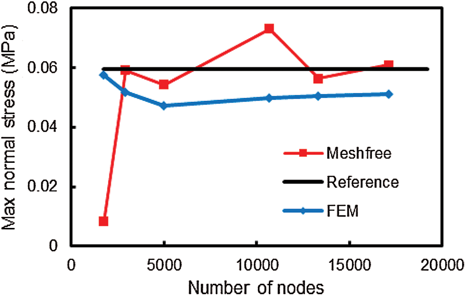
Figure 10: Convergence of maximum normal stress  obtained by EFG and FEM
Figs. 11 and 12 show the displacement distribution along edge 1-2 with respect to X and Z axes, respectively. The X-displacement is the main deformation response of the block. The number of nodes used in the three models is around 17000. The figures show that EFG predicts more accurate solutions than FEM with the same number of DOFs.
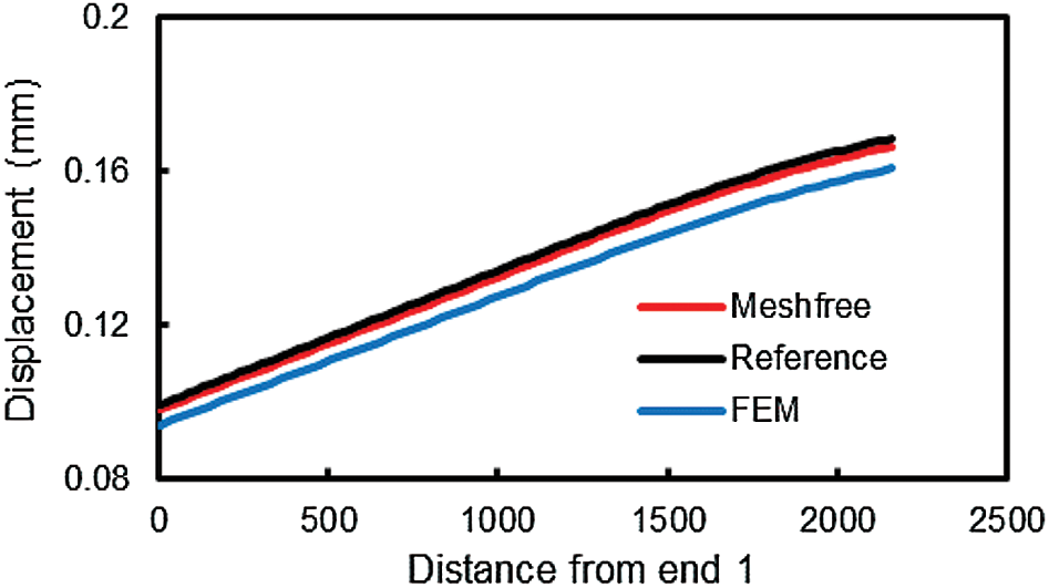
Figure 11: Distribution of X-displacement along edge 1-2
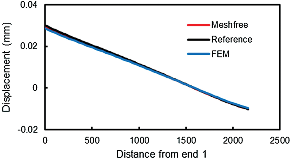
Figure 12: Distribution of Z-displacement along edge 1-2
The distribution of normal stress  is presented in Fig. 13. Although the EFG results are fluctuating, the approximation polynomial (Poly [Meshfree]) derived from EFG’s data shows better agreement with “Reference” than FEM’s line does.
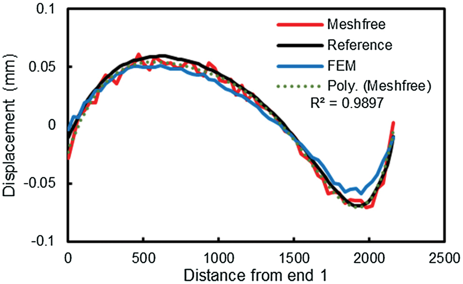
Figure 13: Normal stress distribution along edge 1-2
Fig. 14 illustrates the deformations along X and Z axes of the block. The comparison is performed between the results obtained by meshfree method and those of ANSYS. The solutions show that the difference of maximum X-displacement is 1.2%, while that difference for Z-displacement is 2.1%.
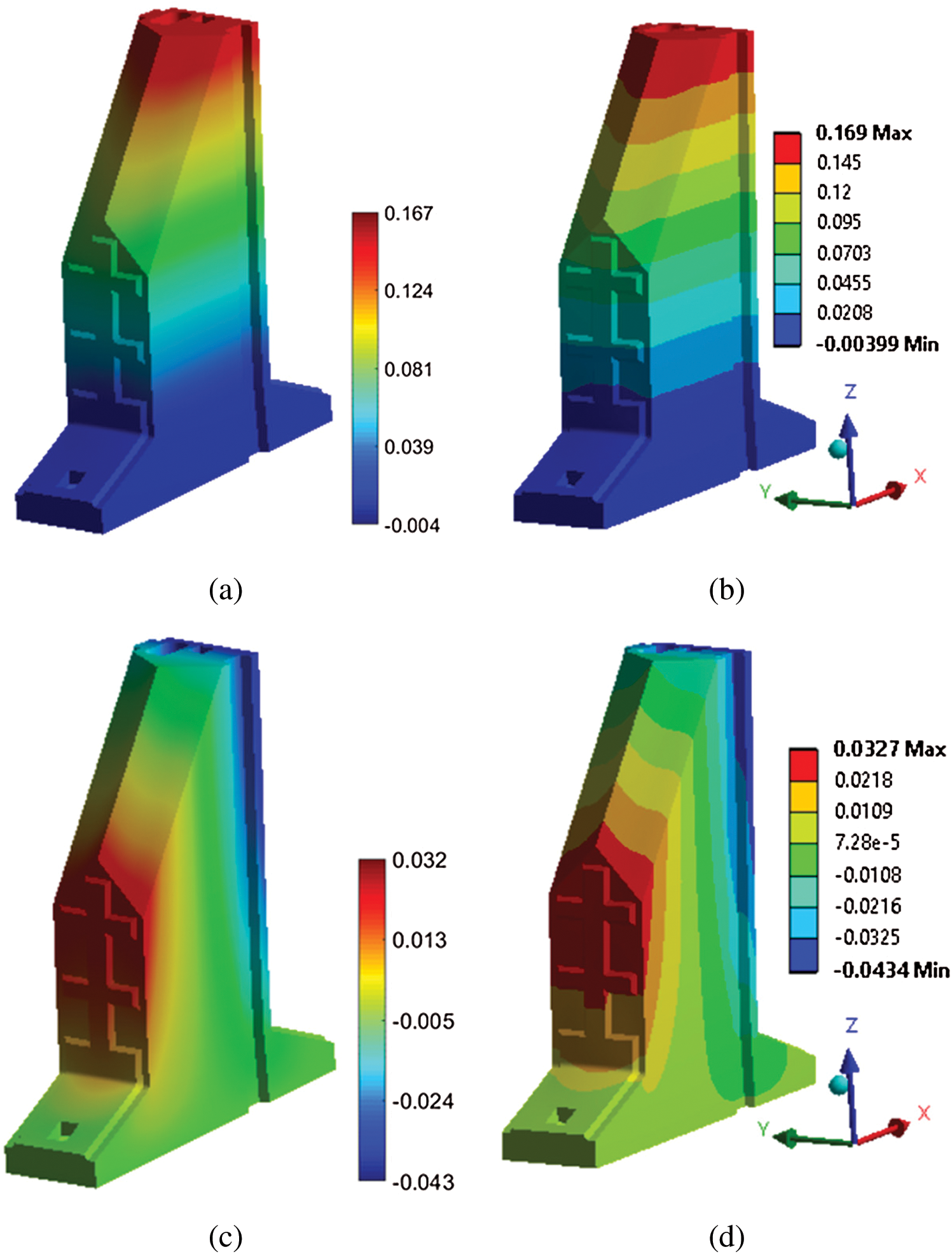
Figure 14: Comparing the deformations of the block analysed by meshfree method with reference results. a) X-displacement by EFG, b) Reference X-displacement, c) Z-displacement by EFG, d) Reference Z-displacement
The EFG meshfree method using three-dimensional moving least square approximation was successfully applied in analyzing three-dimensional complex geometry structures, namely interlocking concrete blocks for step seawall structure. The elastostatic responses of the block were obtained relying on Galerkin weak form formulation over local support domains, which are defined by a collection of discretised nodes in a spherical region. The nodal amount ranging from 10 to 60 was also investigated because of its crucial role in MLS interpolation. The accuracy and efficiency of the studied method were validated by making comparison of the solutions analysed by FEM using linear shape functions on tetrahedral elements and well known commercial software, ANSYS. Some conclusions are pointed out as follows:
•The elastostatic responses of the studied concrete block obtained by EFG method converge faster and are more accurate than those of standard FEM.
•The number of nodes in support domain should be greater than 20 and should be in the range from 30 to 60.
•The singular moment matrix may occur if the nodal number in support domain is less than 20.
Because of just using a number of discretised nodes, the application of EFG method in analysing 3D complex structure is simpler compared to regular FEM.
Acknowledgement: The authors acknowledge the help of ours colleague.
Funding Statement: This work was financial support by the VLIR-UOS TEAM Project, VN2017TEA454A103, ‘An innovative solution to protect Vietnamese coastal riverbanks from floods and erosion’, funded by the Flemish Government. https://www.vliruos.be/en/projects/project/22?pid=3251.
Conflicts of Interest: The authors declare that they have no conflicts of interest to report regarding the present study.
1. M. H. Gu, D. L. Young and C. M. Fan. (2009). “The method of fundamental solutions for one-dimensional wave equations,” Computers, Materials & Continua, vol. 11, no. 3, pp. 185–208.
2. B. J. Gross, N. Trask, P. Kuberry and P. J. Atzberger. (2020). “Meshfree methods on manifolds for hydrodynamic flows on curved surfaces: A generalized moving least-squares (GMLS) approach,” Journal of Computational Physics, vol. 409, pp. 109340.
3. J. Bishop. (2020). “A kinematic comparison of meshfree and mesh-based Lagrangian approximations using manufactured extreme deformation fields,” Computational Particle Mechanics, vol. 7, no. 2, pp. 257–270.
4. G. Kosec and B. Šarler. (2011). “H-adaptive local radial basis function collocation meshless method,” Computers, Materials & Continua, vol. 26, no. 3, pp. 227–253.
5. T. D. Tran, C. H. Thai and H. Nguyen-Xuan. (2018). “A size-dependent functionally graded higher order plate analysis based on modified couple stress theory and moving Kriging meshfree method,” Computers, Materials & Continua, vol. 57, no. 3, pp. 447–483.
6. D. Paquet and S. Ghosh. (2011). “Microstructural effects on ductile fracture in heterogeneous materials. Part I: Sensitivity analysis with LE-VCFEM,” Engineering Fracture Mechanics, vol. 78, no. 2, pp. 205–225.
7. H. Ren, X. Zhuang, T. Rabczuk and H. Zhu. (2019). “Dual-support smoothed particle hydrodynamics in solid: Variational principle and implicit formulation,” Engineering Analysis with Boundary Elements, vol. 108, pp. 15–29.
8. X. Chen, B. Hofland and W. Uijttewaal. (2016). “Maximum overtopping forces on a dike-mounted wall with a shallow foreshore,” Coastal Engineering, vol. 116, pp. 89–102.
9. S. Y. Yu, M. J. Peng, H. Cheng and Y. M. Cheng. (2019). “The improved element-free Galerkin method for three-dimensional elastoplasticity problems,” Engineering Analysis with Boundary Elements, vol. 104, pp. 215–224.
10. A. J. C. Crespo, M. Gómez-Gesteira and R. A. Dalrymple. (2007). “Boundary conditions generated by dynamic particles in SPH methods,” Computers, Materials & Continua, vol. 5, no. 3, pp. 173–184.
11. P. S. Jensen. (1972). “Finite difference techniques for variable grids,” Computers & Structures, vol. 2, no. 1–2, pp. 17–29.
12. T. Zhang and X. Li. (2020). “Variational multiscale interpolating element-free Galerkin method for the nonlinear Darcy–Forchheimer model,” Computers & Mathematics with Applications, vol. 79, no. 2, pp. 363–377.
13. R. Singh and K. M. Singh. (2019). “Interpolating meshless local Petrov-Galerkin method for steady state heat conduction problem,” Engineering Analysis with Boundary Elements, vol. 101, pp. 56–66.
14. M. Abbaszadeh and M. Dehghan. (2020). “Direct meshless local Petrov–Galerkin (DMLPG) method for time-fractional fourth-order reaction–diffusion problem on complex domains,” Computers & Mathematics with Applications, vol. 79, no. 3, pp. 876–888.
15. H. Ren, X. Zhuang, Y. Cai and T. Rabczuk. (2016). “Dual-horizon peridynamics,” International Journal for Numerical Methods in Engineering, vol. 108, no. 12, pp. 1451–1476.
16. H. Ren, X. Zhuang and T. Rabczuk. (2020). “Nonlocal operator method with numerical integration for gradient solid,” Computers & Structures, vol. 233, pp. 106235.
17. H. Mellouli, H. Jrad, M. Wali and F. Dammak. (2020). “Free vibration analysis of FG-CNTRC shell structures using the meshfree radial point interpolation method,” Computers & Mathematics with Applications, vol. 79, no. 11, pp. 3160–3178.
18. L. D. C. Ramalho, J. Belinha and R. D. S. G. Campilho. (2019). “The numerical simulation of crack propagation using radial point interpolation meshless methods,” Engineering Analysis with Boundary Elements, vol. 109, pp. 187–198.
19. L. M. J. S. Dinis, R. M. N. Jorge and J. Belinha. (2007). “Analysis of 3D solids using the natural neighbour radial point interpolation method,” Computer Methods in Applied Mechanics and Engineering, vol. 196, no. 13–16, pp. 2009–2028.
20. B. Ren, H. Wen, P. Dong and Y. Wang. (2016). “Improved SPH simulation of wave motions and turbulent flows through porous media,” Coastal Engineering, vol. 107, pp. 14–27.
21. H. Akbari and M. M. Namin. (2013). “Moving particle method for modeling wave interaction with porous structures,” Coastal Engineering, vol. 74, pp. 59–73.
22. H. Nasiri, M. Y. A. Jamalabadi, R. Sadeghi, M. R. Safaei, T. K. Nguyen et al.. (2019). , “A smoothed particle hydrodynamics approach for numerical simulation of nano-fluid flows: Application to forced convection heat transfer over a horizontal cylinder,” Journal of Thermal Analysis and Calorimetry, vol. 135, no. 3, pp. 1733–1741.
23. F. Almasi, M. S. Shadloo, A. Hadjadj, M. Ozbulut, N. Tofighi et al.. (2019). , “Numerical simulations of multi-phase electro-hydrodynamics flows using a simple incompressible smoothed particle hydrodynamics method,” Computers & Mathematics with Applications, (In Press).
24. J. Dolbow and T. Belytschko. (1998). “An introduction to programming the meshless Element Free Galerkin method,” Archives of Computational Methods in Engineering, vol. 5, no. 3, pp. 207–241.
25. R. Kumar and G. Dodagoudar. (2013). “Element free Galerkin method for two dimensional contaminant transport modelling through saturated porous media,” International Journal of Geotechnical Engineering, vol. 3, no. 1, pp. 11–20.
26. S. Milewski. (2012). “Meshless finite difference method with higher order approximation—applications in mechanics,” Archives of Computational Methods in Engineering, vol. 19, no. 1, pp. 1–49.
27. Q. Li, S. Shen, Z. D. Han and S. N. Atluri. (2003). “Application of meshless local petrov-galerkin (MLPG) to problems with singularities, and material discontinuities, in 3-D elasticity,” Computer Modeling in Engineering and Sciences, vol. 4, no. 5, pp. 571–585.
28. G. R. Liu, G. Y. Zhang, Y. T. Gu and Y. Y. Wang. (2005). “A meshfree radial point interpolation method (RPIM) for three-dimensional solids,” Computational Mechanics, vol. 36, no. 6, pp. 421–430.
29. Z. J. Meng, H. Cheng, L. D. Ma and Y. M. Cheng. (2019). “The dimension splitting element-free Galerkin method for 3D transient heat conduction problems, science China: physics,” Mechanics and Astronomy, vol. 62, no. 4, pp. 40711.
30. H. Cheng, M. J. Peng and Y. M. Cheng. (2018). “The dimension splitting and improved complex variable element-free Galerkin method for 3-dimensional transient heat conduction problems,” International Journal for Numerical Methods in Engineering, vol. 114, no. 3, pp. 321–345.
31. Y. Cheng, F. Bai, C. Liu and M. Peng. (2016). “Analyzing nonlinear large deformation with an improved element-free Galerkin method via the interpolating moving least-squares method,” International Journal of Computational Materials Science and Engineering, vol. 5, no. 4, pp. 1650023.
32. Z. J. Meng, H. Cheng, L. D. Ma and Y. M. Cheng. (2019). “The hybrid element-free Galerkin method for three-dimensional wave propagation problems,” International Journal for Numerical Methods in Engineering, vol. 117, no. 1, pp. 15–37.
33. Z. Zhang, D. M. Li, Y. M. Cheng and K. M. Liew. (2012). “The improved element-free Galerkin method for three-dimensional wave equation,” Acta Mechanica Sinica/Lixue Xuebao, vol. 28, no. 3, pp. 808–818.
34. S. Garg and M. Pant. (2018). “Meshfree methods: A comprehensive review of applications,” International Journal of Computational Methods, vol. 15, no. 4, pp. 1830001.
35. P. Lancaster and K. Salkauskas. (1981). “Surfaces generated by moving least squares methods,” Mathematics of Computation, vol. 37, no. 155, pp. 141.
36. G. R. Liu and Y. T. Gu. (2005). An Introduction to Meshfree Method and Their Programming, 1st ed., Henderson, NV.
37. H. Nguyen-Ngoc, P. Phung-Van, B. L. Dang, H. Nguyen-Xuan and M. A. Wahab. (2019). “Static and dynamic analyses of three-dimensional hollow concrete block revetments using polyhedral finite element method,” Applied Ocean Research, vol. 88, no. 3, pp. 15–28.
 | This work is licensed under a Creative Commons Attribution 4.0 International License, which permits unrestricted use, distribution, and reproduction in any medium, provided the original work is properly cited. |