DOI:10.32604/cmc.2020.012688
| Computers, Materials & Continua DOI:10.32604/cmc.2020.012688 | |
| Article |
Prediction of Melt Pool Dimension and Residual Stress Evolution with Thermodynamically-Consistent Phase Field and Consolidation Models during Re-Melting Process of SLM
1Department of Aerospace Engineering, Seoul National University, Seoul, 08826, South Korea
2Institute of Advanced Aerospace Technology, Seoul National University, Seoul, 08826, South Korea
*Corresponding Author: Gun Jin Yun. Email: gunjin.yun@snu.ac.kr
Received: 09 July 2020; Accepted: 17 August 2020
Abstract: Re-melting process has been utilized to mitigate the residual stress level in the selective laser melting (SLM) process in recent years. However, the complex consolidation mechanism of powder and the different material behavior after the first laser melting hinder the direct implementation of the re-melting process. In this work, the effects of re-melting on the temperature and residual stress evolution in the SLM process are investigated using a thermo-mechanically coupled finite element model. The degree of consolidation is incorporated in the energy balance equation based on the thermodynamically-consistent phase-field approach. The drastic change of material properties due to the variation of temperature and material state is also considered. Using the proposed simulation framework, the single-track scanning is simulated first to predict the melt pool dimension and validate the proposed model with the existing experimental data. The obtained thermal histories reveal that the highest cooling rate is observed at the end of the local solidification time which acts as an important indicator for the alleviation of temperature gradient. Then, the scanning of a whole single layer that consists of multiple tracks is simulated to observe the stress evolution with several re-melting processes. After the full melting of powder material in the first scanning process, the increase of residual stress level is observed with one re-melting cycle. Moreover, the predicted stress level with the re-melting process shows the variation trend attributable to the accumulated heat in the tracks. The numerical issues and the detailed implementation process are also introduced in this paper.
Keywords: Selective laser melting; thermo-mechanical analysis; Ti-6Al-4V; additive manufacturing; re-melting; residual stress
The additive manufacturing (AM) process is an advanced manufacturing technique to build a three-dimensional part using computer-aided-design (CAD) with successive melting/fusing/curing processes of distributed raw material on a solid substrate. Among the AM processes defined by ASTM [1], selective laser melting (SLM) is one of the powder bed fusion (PBF) processes where the metallic powder is melted and fused by a high power-density laser to build a part. In recent years, SLM has gained significant attention owing to its ability to fabricate metallic parts with complex geometries and added functionalities [2]. Furthermore, the layer-by-layer manufacturing approach of SLM enables quicker production compared to the conventional manufacturing process. The full melting of powder during the SLM process also leads to a near full density (99.9%) of the printed part with various metallic materials [3]. Therefore, SLM is now one of the most commercialized PBF processes used in several core manufacturing industries including automobile, aerospace, biomedical, and energy industries [4–8].
Despite the advantages of the SLM process, the inability to fully observe and model the complex nature of the process hinders the wide implementation of SLM. During the SLM process, highly concentrated heat energy induced by a laser beam is absorbed by powder particles leading to localized melting which forms a molten region called melt pool. Then, the rapid consolidation of the molten material occurs as the center of the heat source moves to the scanning direction. The heating and the consolidation mechanism in the SLM process include various physical phenomena (melting, vaporization, and melt pool dynamics such as Marangoni convection) [9]. The short interaction time and rapid consolidation ( K/s) [10] also makes it challenging to manage and optimize the process. For instance, the high cooling rate and steep temperature gradient due to the short powder-laser interaction time cause residual stress and distortion in the printed products. For an SLM processed part, residual stress is the main cause of failure which could lead to cracks that weaken the mechanical properties of the part as reported by [11–13]. Furthermore, the unstable geometry of the melt pool due to the improper selection of process parameters could induce the formation of the balls (which is called ‘balling effect’) and increases the surface roughness as well as the porosity [14].
To mitigate these defects and improve the mechanical properties of the SLM printed parts, laser re-melting procedure has been employed as a solution. Yasa et al. [15] studied the influence of re-melting on the density and the surface quality of SLM printed 316L stainless steel and Ti-6Al-4V parts. They reported that the re-melting process improves the density to near 100% and reduces the surface roughness about 90%. Shiomi et al. [16] applied the re-scanning process during the SLM process of 316L stainless steel and proved that the residual stress is relieved with 150% of the forming energy. On the other hand, laser re-melting does not always lead to the enhancement of the quality of the SLM printed part. Kruth et al. [17] applied the post scanning process with the same scan pattern and spot size during the fabrication of Ti-6Al-4V parts. They found out that only the re-scanning process with low scan speed can reduce the residual stress. They concluded that the laser re-melting with high scanning speed rather increases the residual stress due to the high thermal gradient. Furthermore, Wei et al. [18] demonstrated that the one cycle of re-melting even led to an increase of residual stress due to the less amount of absorbed energy after the densification of powder material. These results show that the laser re-melting should be carefully applied considering the process parameters and the heat transfer mechanisms of the SLM process.
In recent years, numerous numerical models have been proposed and used to investigate the temperature and stress evolutions during the SLM process as well as the effect of the process parameters on the quality of the printed part. Simulation methods with various scales have been proposed from the mesoscale approach that considers individual powder particles to macroscale analysis with an entire part geometry. Chen et al. [19,20] proposed a numerical model to investigate the fundamental mechanisms of the powder packing in the PBF process based on the discrete element method (DEM). Khairallah et al. [21] proposed a 3D mesoscopic model that couples thermal diffusion to hydrodynamics using the ALE3D multiphasic code with a finite volume formulation. Yan et al. [22] proposed a multi-physics powder-scale model of PBF process to study the physical mechanisms of track defects. The continuum-based finite element method (FEM) has also been a promising technique to study the SLM process. Fu et al. [23] proposed a multilayer microscale SLM model with a surface moving heat flux considering the phase and temperature-dependent material properties of Ti-6Al-4V. Their predictions of molten pool geometry and dimensions were validated using the experimentally measured melt pool geometry. Gusarov et al. [24] proposed an analysis model of laser beam interaction with the 316L stainless steel powder bed on a solid substrate. The authors explained the “balling effect” by the Plateau-Rayleigh capillary instability and studied the melt pool geometric characteristics that stabilize the process. Hussein et al. [25] presented a transient three-dimensional finite element thermo-mechanical model of the SLM process to predict the temperature and stress fields a single layer of 316L stainless steel. In their simulation results, the highest temperature gradient was observed at the beginning of the scanning track and high cooling rates were predicted on solid substrate rather than loose powder bed. Parry et al. [26] proposed a coupled thermo-mechanical simulation to understand the effect of laser scan strategy on the formation of residual stress in the SLM process. Foroozmehr et al. [27] developed a three-dimensional finite element model for SLM process simulation which takes into account optical penetration depth (OPD) of the laser beam into the powder. The proposed heat source model was first calibrated with existing experimental data and then was validated by measured melt pool dimension in the subsequent experiment. Roy et al. [28] established a novel heat transfer model for the SLM process considering the degree of consolidation using multiple state variables to track melting, consolidation, and re-solidification process. The proposed model considers the effect of the consolidation that leads to the reduction of absorbed laser power into the material.
Although there have existed considerable efforts to study and optimize the SLM process, the thermal history and the consolidation behavior with the re-melting process have not been studied in detail. To investigate the heat transfer mechanisms and the generation of residual stress with several re-melting cycles, a numerical approach could be an effective solution to provide an insight into the process. However, most of the previous studies seldom consider (or partially apply) the drastic change of material properties and the degree of consolidation which can lead to insufficient reflection of the actual process. Furthermore, the computational issues and implementation methods in finite element analysis also have not been introduced in detail.
In this study, a simulation framework for the thermo-mechanical analysis of the SLM process considering the temperature-dependent material properties, and the degree of consolidation is proposed using commercial finite element analysis software ABAQUS. A heat transfer model based on the phase-field approach considering the consolidation behavior and latent heat of vaporization is implemented with the provided user-subroutines. The proposed model is then validated with the simulation results of the single-track scanning process using the experimentally measured melt pool dimensions from existing results. Then, a single-layer scanning process with several re-melting cycles is simulated and the stress field is obtained by conducting sequentially coupled thermo-mechanical analysis. The model considers the strain hardening and the annealing effect with the element deactivation techniques applied to the powder state material. The different heat absorption mechanisms for the powder and dense state material are also considered using both of the surface and volumetric heat flux models. Finally, the variation of the stress level and the cooling rate after the local solidification with the several re-melting processes are discussed to evaluate the process.
To build a numerical model of the SLM process, complex physical phenomena including the moving heat flux, the phase change, and the consolidation of the powder material with severe temperature change must be considered. The consolidated material can undergo several heating cycles and be re-melted as the laser beam passes the neighboring region during the process. Furthermore, the thermal and mechanical properties of each material state (powder, liquid, and solid) are significantly different from one another. In this section, the numerical models for the thermo-mechanical analysis of SLM are described including the governing equations for continuum-based finite element formulations, the reference heat source models, thermal and mechanical material properties with effective values for powder/liquid states.
2.1 Thermal Equilibrium Equation Based on Phase-Field Approach
In this study, the powder bed is treated as a continuum material with effective material properties. The fluid dynamic is not considered thus the melt flow and the recoil pressure due to the vaporization are neglected for the following thermo-mechanical analysis. The governing equation of heat transfer which is the energy balance equation for an arbitrary material point in a volume  is given by


where  is the energy density,
  is the heat flux vector,
  is the coordinate vector,
  is the volumetric internal heat generation rate,
  is the thermal conductivity, T is the temperature, and
  represents the time. In the SLM process,
  becomes the heat-induced by the laser.
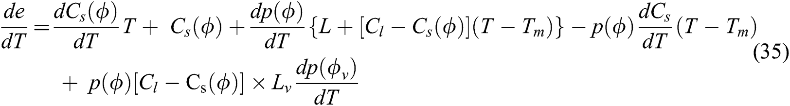
Wang et al. [29] proposed thermodynamically-consistent phase-field models for solidification based on an entropy functional. The concept of phase-field function is then adopted by Roy et al. [28] in the form of an energy balance equation with state variables to model the consolidation behavior of the material in the SLM process. The energy density  in terms of
  and material properties determined by the state variables
  and
and  defined by as follows

where  is the volumetric heat capacity in solid-state,
  is the volumetric heat capacity in the liquid state,
  is the latent heat of fusion,
  is the average melting temperature which is the average value of the liquidus temperature
  and the solidus temperature
  . The function
  is a polynomial form of the phase parameter
  which satisfies the required conditions that
 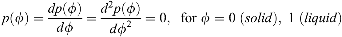 to have local minima of Helmholtz free energy density for solid and liquid states given by

The phase parameter  and the consolidation parameter
  are defined as follows


where  if
if  ,
,  if
if  , and becomes a value between 0 and 1 when
  . A is the parameter that determines the steepness of change which is 5.0 in this study for the smooth transition.
  represents the degree of consolidation which is related to the history of the phase parameter (which holds the maximum value of
  ) in each material point. The volumetric heat capacity of solid-state
  and the thermal conductivity
  are determined by the degree of consolidation
  as follows


where  and
and  are the porosity and the initial porosity of the powder,
  is the heat capacity of the dense material,
  and
and  are the thermal conductivities of the powder material and dense material.
Lastly, the vaporization term is added in the energy density Eq. (3) to consider the latent heat of vaporization with the corresponding phase parameter as follows


where  is the latent heat of vaporization,
  is the vaporized temperature,
  is the liquidus temperature at the liquid-vapor transition,
  is the average vaporization temperature, and
  if
if  to indicate whether the material is vaporized or not. The vaporized region is then treated as empty space with zero conductivity with sufficient large heat capacity to limit the excessive rise of the temperature.
The material properties required for SLM process simulation are highly dependent on the temperature and the material state due to the severe temperature fluctuation. The recommended thermophysical properties are often used with some uncertainties near or above the melting temperature as reported by many previous studies [30–32]. In particular, the effective thermal conductivity of the loose metallic powder is dependent on the void fraction, powder size, and powder morphology rather than the material itself which is often assumed as a small value compared to that of the dense state as in the previous study [33]. In this paper, 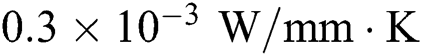 is taken for the conductivity of the powder state and the linearly extrapolated value made up to the melting point is used for the conductivity of dense material
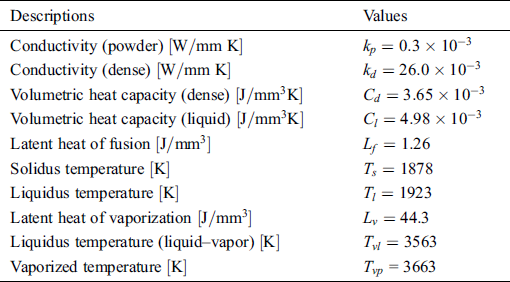
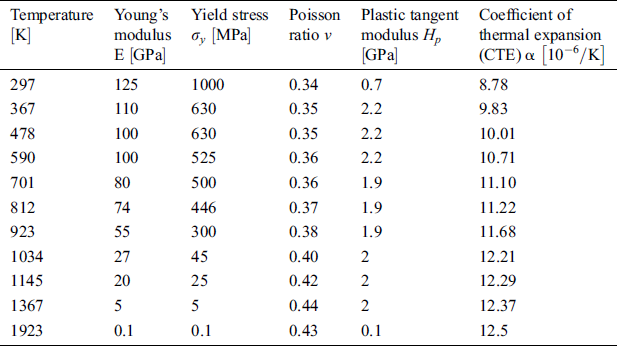
  . In this study, we consider Ti-6Al-4V with the material properties as listed in Tab. 1 [30–32,34–36].
Table 1: Thermal Properties of Ti-6Al-4V
2.2 Boundary and Initial Conditions
The main heat transfer mechanism in the SLM process consists of heat radiation to the powder layer from the laser beam, heat conduction, and heat convection at the free surface. The typical boundary and initial conditions for the SLM process are shown in Fig. 1. The heat transfer equation for a system is supplemented by following initial and boundary conditions
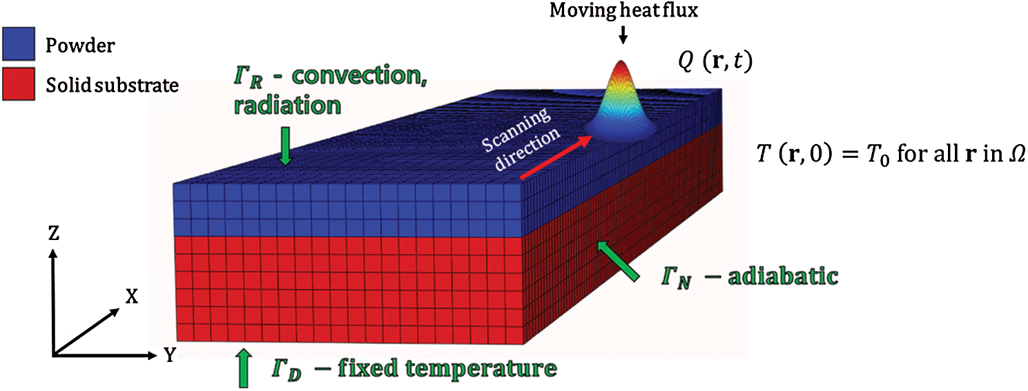
Figure 1: Typical boundary and initial conditions for finite element analysis of the SLM process


where  is the initial temperature which is the ambient temperature (
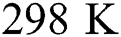 ),
),  is the convection coefficient,
  is the Stefan-Boltzmann constant, and
  is the emissivity. Dirichlet boundary condition of
  is applied to
  , which is the contact area of the substrate the build plate with. Neumann boundary conditions where the specified heat flux
  (adiabatic) is applied to
  which is the lateral surfaces. Lastly, Robin or convective boundary condition with radiation is applied to
  which is the free surface. The radiation loss has been often neglected for SLM process simulation in the many previous studies [25,37–39] because it does not affect the simulation accuracy significantly but increases the complexity due to its nonlinearity. Thus, only the convective boundary condition with
  on the free surface is considered in this study.
For the simulation of the SLM process and other laser beam applications, numerical heat source models are widely used to model the moving laser beam. In the numerical model, the laser beam is modeled as a moving heat flux determined by the distance from the center of the virtual beam and other required beam parameters including the laser spot diameter and the scanning velocity.
The representative numerical heat source models are generally divided into 2 types (2D or 3D) as shown in Tabs. 2 and 3. The models can be used considering the different optical penetration depth of materials. For example, the optical penetration depth is about tens of nanometers for dense material [40]. Thus, it is reasonable to use the surface heat flux models for the dense state material. But to consider the optical penetration through the porous material, 3D volumetric heat source models can be used to apply volumetric heat flux.
Table 2: Numerical heat source models—surface (2D) heat flux
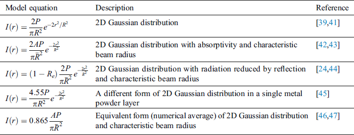
Table 3: Numerical heat source models—volumetric (3D) heat flux
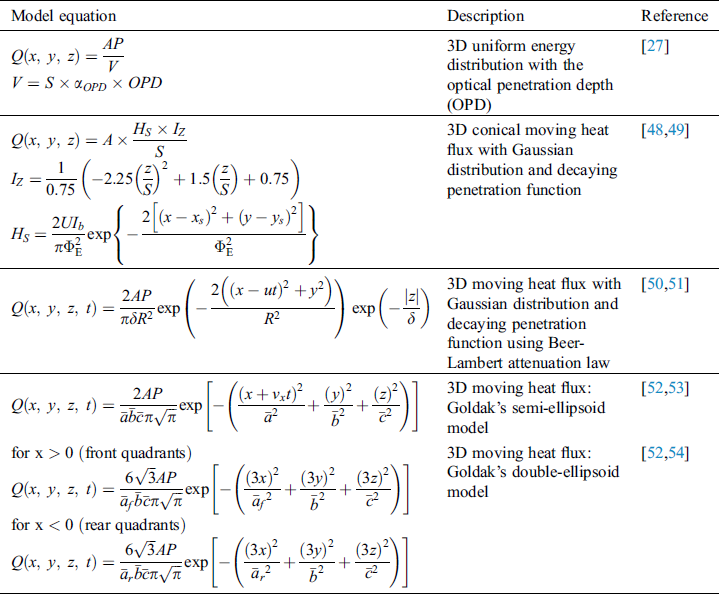
The penetration depth and the other geometric parameters for volumetric heat source models are often determined empirically and need calibration process which requires some experimental results beforehand. Moreover, the obtained temperature fields based on these models are highly affected by the geometric shape of the heat source rather than the applied process parameters and the absorption mechanisms.
In order to obtain a more analytical solution of the heat flux in the SLM process, Gusarov et al. [24] solved the radiation transfer equation taking into account the scattering of the laser beam through the porous material. The dimensionless form for the fraction of the absorbed energy through the porous medium is as follows
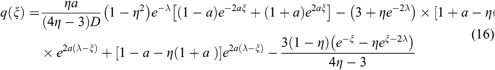


where  is the extinction coefficient,
  is the mean diameter of the particles,
  is the layer thickness,
  is the optical thickness,
  is the dimensionless coordinate, and
  is the hemispherical reflectivity which is assumed as 0.7 in this study. Then, the volumetric heat source due to the radiation absorption can be written as follows with the Gaussian distributed laser energy and the consolidation parameter
  to consider the less amount of absorbed energy for the dense and molten state of the material.


In addition, the 2D Gaussian distributed heat flux is applied at the top surface with the absorptivity  of 0.3 for re-melting processes assuming full melting and consolidation of the material after first scanning.
The governing equation for static structural analysis which is the conservation of linear momentum equation is expressed as follows

where  is the body force vector and
  is the Cauchy stress tensor. Neglecting the body force, only the first term remains in the Eq. (24) for further finite element formulations. The mechanical constitutive law is given as

where  is the linear elastic fourth-order material stiffness tensor,
  is the total strain tensor and
  ,
,  , and
, and  are the elastic, plastic, and thermal strain tensors respectively. For the elastoplastic constitutive material model, isotropic and kinematic hardening models are generally adopted in the SLM process simulations. In this paper, the isotropic hardening model with Von Mises yield function is used which is given as


where  is the yield function,
  is the Mises’ stress,
  is the isotropic hardening stress,
  is the yield stress,
  is the deviatoric stress tensor, and the plastic strain increment according to the plastic flow rule is as follows

where  is the plastic multiplier which is the increment in equivalent plastic strain
  for VonMises material. For an incremental formulation, the current stress
  can be updated using the previous stress
  , and the stress increment
  as follows

If  < 0 (i.e., within linear elastic range), the stress is updated without plastic strain increment.

If  > 0 (i.e., out of the linear elastic range), the stress is updated with plastic strain increment as follows

The mechanical properties of solid Ti-6Al-4V used in this study are listed in Tab. 4 (interpolating and extrapolating the values reported in the previous studies [47,55–58]). For powder and liquid states, the stiffness of the material is negligible compared to the stiffness of the dense solid-state. Thus, a small value ( ) compared to the value of the dense solid-state under room temperature (125
  ) is used for the powder stiffness to make it virtually zero (deactivated), but not exactly zero to guarantee a positive definite stiffness matrix. The negligible yield stress at the melting temperature is set to be
  [26] with perfect plasticity to consider the annealing effect (equivalent plastic strain is reset to zero to remove the hardening memory) [59] at the liquidus temperature.
Table 4: Mechanical properties of Ti-6Al-4V
3 Implementation with Finite Element Method
To obtain the predictions for temperature and stress fields in the SLM process, including subsequent results such as melt pool dimensions and residual stress field, a sequentially coupled finite element analysis framework is developed using the commercial software ABAQUS/Standard. ABAQUS provides the interface for programming user-defined material behavior and boundary conditions. The specific features and numerical models of SLM introduced in Section 2 are implemented using the provided user subroutines [60]. The flow chart for the thermo-mechanical analysis of the SLM process with relevant user subroutines is shown in Fig. 2. First, thermal analysis is conducted to obtain the temperature field with defined geometry, mesh, and 3D thermal finite element (DC3D8). Then, the transient temperature field is passed to the subsequent mechanical analysis as a predefined field. The same geometry and mesh, but different element type (C3D8) are used in the mechanical analysis to obtain the stress and deformation induced by the thermal expansion. The state variables that are dependent on temperature histories are updated at every time increment. The implementation process and programmed user subroutines for each analysis are described with relevant computational issues in this section.
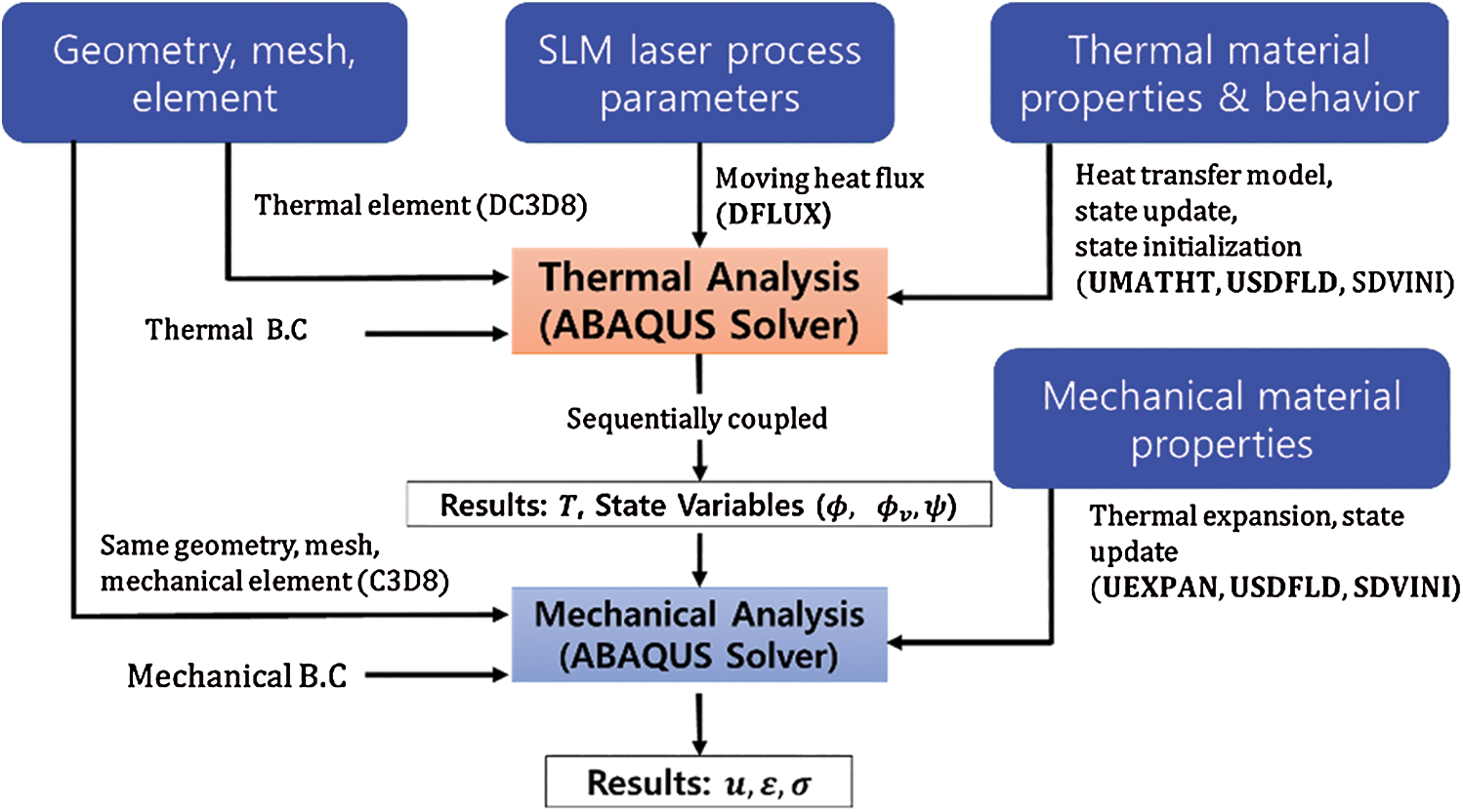
Figure 2: Flow chart for sequentially coupled thermo-mechanical analysis for SLM process in ABAQUS/Standard, (∙): user subroutines
The heat source can be modeled using DFLUX subroutine in ABAQUS. The position of the flux integration point is passed to the subroutine and the distance from the center of a virtual laser beam needs to be calculated to use the heat source models introduced in Section 2.3. The unit of the heat flux is  for the surface heat flux and
  for the volumetric heat flux.
The variational statement of the energy balance equation (a 1D problem for simplicity) and the Jacobian (or tangent stiffness) contributions of each term after time integration using the backward difference in ABAQUS/Standard is as follows [59]

and the linearized equation using Newton’s method with the convection boundary condition is
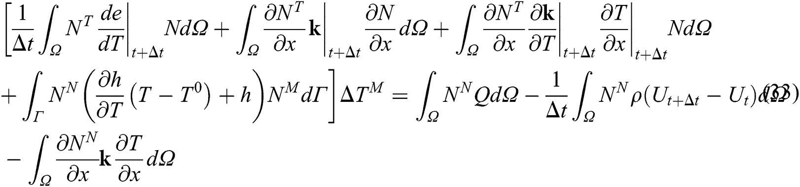
where  is the density,
  is the arbitrary variation field,
  is the conductivity matrix,
 is the incremental correction of temperature,
  is the time increment,
  and
and  are the interpolation function matrices. ABAQUS/Standard uses Newton’s method to solve the nonlinear equation. To define user-defined thermal constitutive behavior of the material, UMATHT subroutine is written in FORTRAN to define and update the following variables: energy density
  , the variation of energy density to temperature
  , the heat flux vector
 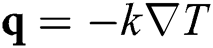 , the variation of the heat flux vector to temperature
  , and the variation of the heat flux vector to the spatial gradients of temperature
  which is the conductivity
  . To use the temperature and temperature history-dependent state variables in the energy density Eq. (3), the USDFLD subroutine is used to update and save the state variables described in Section 2.1 for every iteration.
Because the state variable  in the equation changes only when the new maximum value of
  is obtained, the derivative of relevant variables at time
  has zero or nonzero values according to the variation of
  . For instance, the derivative of the internal energy density to the temperature is as follows
Case 1. when  is not updated

Case 2. when  is updated with current
It is worth noting that different forms of energy balance equation based on thermodynamic consistency can be implemented in the same way. To validate the model implemented in ABAQUS, the variation of energy density at a material point (for both initially porous and dense cases) with temperature is extracted as shown in Fig. 3. The initial state of the material point is applied using the SDVINI subroutine which is called at the beginning of the analysis. The result shows that the obtained energy density curves have both the solid-liquid transition and the liquid-vapor transition with a steep increase of the energy density due to the corresponding latent heat values.
Figure 3: Energy density e curves with temperature extracted from a material point in ABAQUS
The time increment also needs to be carefully determined to obtain proper results depending on the choice of the fixed domain methods to solve the phase change problems. The time required for melt interface to reach the steady-state is on the order of  s [28]. If the time increment gets bigger than this unit, the result can significantly differ from the analytical solution due to the big temperature increment especially when using a numerical technique like the equivalent heat capacity method. For this reason, the enthalpy method is usually preferred to consider the enthalpy change due to the phase change [61]. In this study, the variation of energy density is analytically computed using the energy density function Eq. (3) tracking the change of state variables. Also, a laser beam with a constant scanning speed of 200
 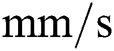 travels 0.2
  in
in  which is 130 times smaller than the laser beam radius 26
  considered in this study. Thus, a maximum time increment of
  selected as a reasonable value for the thermal analysis.
For predictions of stress field and deformation in the SLM process, the temperature field obtained in the previous thermal analysis is passed as a function of time to the mechanical analysis. The time increment can be controlled differently because the convergence criteria are now different from the previous thermal analysis. Besides, it is possible to use a fixed time increment for both thermal and mechanical analysis, but not preferred when the problems are highly nonlinear. For the case of the single-track scanning process considered in this study, the time required for solidification in SLM is generally in the units of  (Section 4.1.2). Also, the rapid decrease of temperature just after the solidification does not affect the stress evolution significantly due to the low modulus value at high temperature (Tab. 4). Thus, the maximum time increment of
  which is 10 times larger than the increment in thermal analysis is used in the mechanical analysis to reduce the computation time.
As the state variables are updated and saved using USDFLD subroutine in the previous thermal analysis, the state variable is used as an additional field variable to apply state-dependent elastic and plastic properties with the annealing temperature as introduced in Section 2.4. To define the thermal expansion induced by the temperature variation, UEXPAN subroutine is used to apply isotropic thermal strain increment with temperature-dependent CTE.
3.3 Dimensions of the Model for the Single-Layer Scanning Process
To validate the analysis methodology introduced in this paper, an SLM process with a single powder layer is simulated. The finite element model with the given initial material states for analysis is as shown in Fig. 4. The 8-node hexahedral element is applied for the entire analysis domain with the dimensions of  . The fine mesh size of
  is applied for the scanning region with a width of 0.5 mm and a track length of 2 mm. According to the previous study [62], the characteristic length of
  is reported as the suitable mesh size that guarantees mesh convergence in the previous study. Furthermore, the meshing for the solid substrate is biased with a higher density towards the powder layer. because the bottom surface is far from the laser-irradiated top surface.
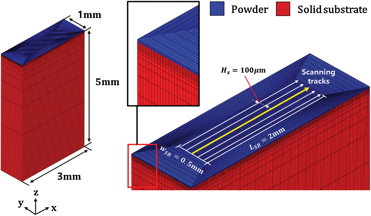
Figure 4: Three-dimensional finite element model for SLM process a) geometry and mesh design, b) top view of model with multiple scanning tracks (yellow track is for the single-track scanning simulation and the 3rd track for the multi-track scanning simulation)
Based on the fact that the selective laser melting process is a sum of single-layer formations, and the thermal cycles of the previous layers have little influence on the temperature profile of subsequent layers [23], the analysis of single-layer scanning can provide quantitative and qualitative features of the SLM process. In this section, the single-track scanning process is analyzed first and the result is quantitatively compared with the experimentally measured melt pool dimensions. Then, the multi-track scanning process is simulated with the predefined scanning paths as shown in Fig. 4 to investigate the stress evolution in the qualitative approach.
The proposed thermal model is validated by comparing the predicted melt pool dimensions with the experimentally results obtained in the literature [35] with various laser powers from 20 to 80 W. The laser beam process parameters used in the analysis are listed in Tab. 5. The obtained phase field for the given cases is illustrated in Fig. 5. The gray color denotes the region where the temperature exceeds the vaporized temperature, the pink color denotes the molten region, the blue color denotes the powder material and the red color denotes the solid substrate. The results show that as the power increases, the size of the melt pool also increases and even material vaporization occurs for the higher laser powers. Besides, the vaporization of alloy with excessive heat input can lead to keyhole-mode melting [63] resulting in lower surface quality and degradation of mechanical properties [64,65] which is not preferred in SLM process. The predicted melt pool width  and the depth
  are compared with the experimentally measured melt pool dimensions. The graphs in Figs. 6 and 7 show the proposed model with the phase field approach which considers the degree of consolidation and the vaporization can predict the melt pool dimension with reasonable accuracy. However, a different trend is observed for the simulation without consolidation and vaporization that the predicted melt pool size increases almost linearly with the laser power increment. Even though the consolidation of material and the latent heat of fusion/vaporization are sometimes neglected for simplicity as reported in many previous studies [23,25,26,28,54], this result shows that they significantly influence the analysis results. However, other important mechanisms related to the vaporization including the surface depression with the recoil pressure, and the multiple reflections of the laser beam are not considered in this study assuming the vaporization is not very severe with the maximum melt pool depth around
  . If intense surface depression with the formation of a deeper melt pool takes place, effective absorptivity may increase rapidly as reported by Trapp et al. [66]. However, consideration of the keyhole mode melting is not the scope of this work. The effective thermal finite element analysis model which captures the keyhole mode melting with effective absorptivity is suggested for future work.
Figure 5: Phase-field in the y-z cross-section with various laser powers a) P = 20 W, b) P = 40 W, c) P = 60 W, d) P = 80 W
Figure 6: Comparison of the predicted melt pool width with the experimental results
Figure 7: Comparison of the predicted melt pool depth with the experimental results
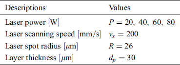
Table 5: Laser beam process parameters for the single track scanning process
4.1.2 Transient Temperature Field and Solidification
The local temperature evolution with the high cooling rate is the key feature of the PBF process which is closely related to the mechanical properties of the SLM printed part and the process stability. The typical local temperature history in the SLM process is as shown in Fig. 8. After the temperature of the local heated point reaches the maximum as the heat source moves, the heat is transferred rapidly to the surroundings due to the high-temperature gradient. Besides, the liquid state is kept at the melting temperature until the latent heat is fully released and this process is called the local solidification as introduced by [67].
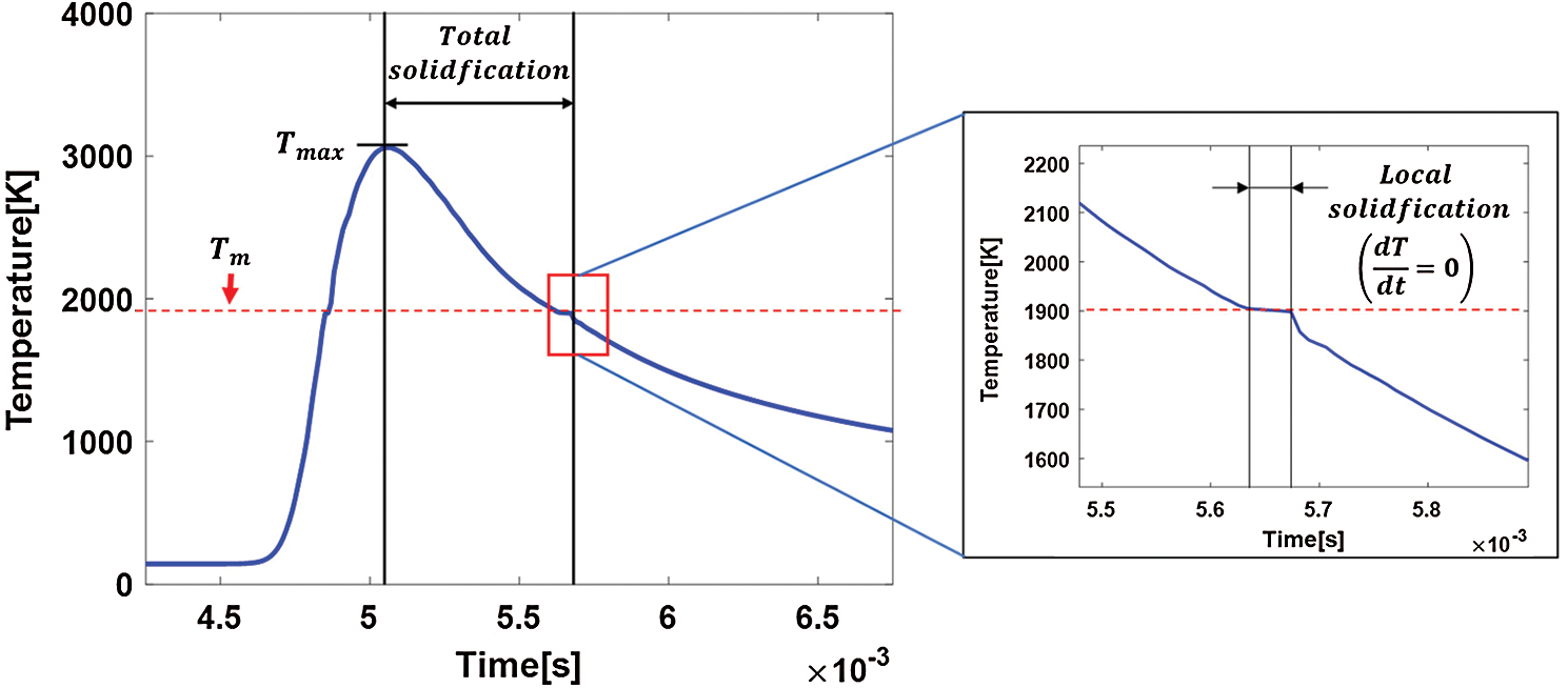
Figure 8: Typical temperature evolution during the SLM process with melting- solidification (total solidification and local solidification)
The transient temperature field, the cooling rate, and the state variables versus time at the middle point of the single-scan track on the solid substrate (which is initially porous) with the varying laser power are depicted in Fig. 9. As more laser power is applied, the maximum temperature increases until it reaches the vaporized temperature when P = 80 W. The cooling rate is computed by the temperature change in a time increment (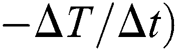 . The negative cooling rate means the temperature is increasing and the graphs show that the increase of the laser power leads to more rapid heating with the minimum cooling rate of
  when P = 80 W. In contrast, the positive cooling rate means the temperature is decreasing because the position is out of the radius of the moving laser beam. The maximum cooling rate of
 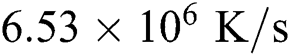 is achieved with the laser power of
  right after the local solidification time. This result shows that the increase of the laser power can help to reduce the cooling rate, as well as mitigating the high-temperature gradient. However, it is worthy to know that the increase of the laser power can lead to keyhole-mode melting and the defects related to material vaporization as reported by [63].
Figure 9: Transient temperature field (blue), cooling rate (black) and state variables:  (red),
  (dotted cyan) and
  (magenta) with laser powers (20–80 W) versus time
The material state can be tracked using the adopted state variables as shown in Fig. 9. When the state variables  and
and  are 0, the material is in the powder state that is not melted and consolidated at the beginning. As the temperature rises with the applied heat flux, both of the state variables become 1 as defined in Section 2.1, which means the material point is in the liquid state at this time. Then, the phase parameter becomes 0 with
  as the material cools down, which indicates that the material is now in the dense solid-state. Furthermore, the temperature reaches the vaporized temperature as more laser power (80 W) is applied. In this case, the material point is vaporized (
 ) after the laser scanning as the latent heat of vaporization is absorbed.
The liquid lifetime can be observed using the state graph as shown in Fig. 9 which is also an important parameter that determines the stability of the track formation as stated by [68]. The liquid lifetime with the laser power of  is
is  ms and increases to
  with the laser power of
  . However, the liquid lifetime decreases to 24 ms when P = 80 W due to the vaporization of the material. This result shows that the increase of laser power contributes to a stable and optimal process to a certain degree where intense vaporization is avoided. The result also implies that the change of the laser power and the other process parameters can yield different outcomes depending on the corresponding region of the process window.
After conducting the simulation of the single-track scanning process, a simulation of a single layer scanning process with multiple scanning tracks is conducted to obtain the stress fields involving several re-melting processes. The laser tracks are defined as shown in Fig. 4 with the process parameters: laser power of 200 W, laser spot radius of 60  , scanning speed of 1000 mm/s, hatch spacing of 100
  , and layer thickness of
  which resembles the process parameters applied in the literature [18].
The single-layer scanning process which involves 0–3 re-melting processes are defined as SLM + LR0, SLM + LR1. SLM + LR2, and SLM + LR3 in this study. For the scanning process of one layer and each re-melting process, the scanning time of 0.01 s is applied. Fig. 10 shows the temperature evolution and the obtained melt pool shape for each scanning process. The results show that a relatively larger and longer melt pool is predicted for the SLM + LR0 case compared to the cases with re-melting processes. This can be explained by the lower absorptivity of the material which turns into the dense state after the first scanning process. Furthermore, as the re-melting process is repeated, more heat is accumulated in the part as shown in Figs. 10b–10d.
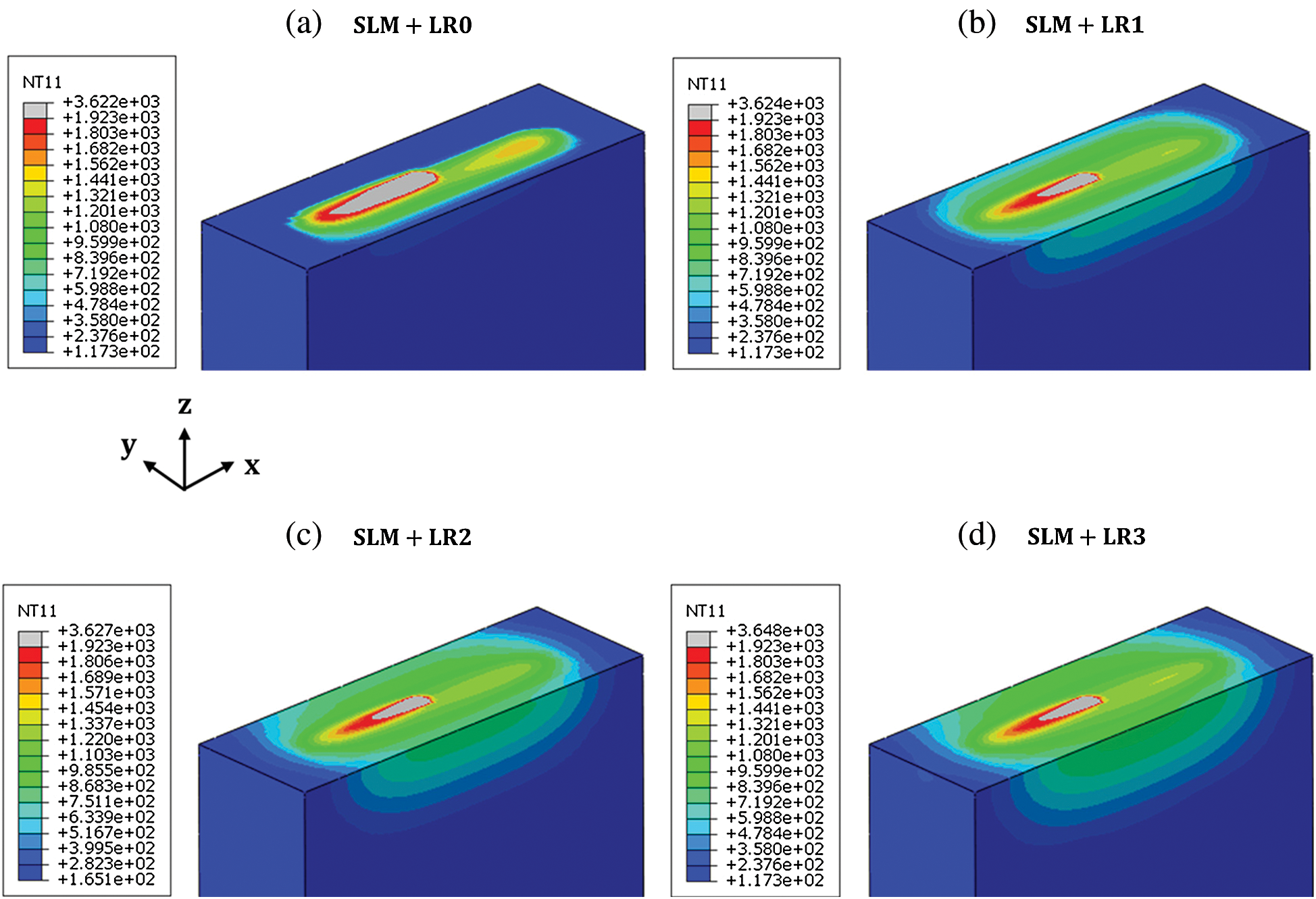
Figure 10: Temperature evolution with the different number of re-melting processes. a) SLM + LR0 (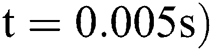 , b) SLM + LR1 (t = 0.015 s), c) SLM + LR2 (t = 0.025 s), d) SLM + LR3 (t = 0.035 s)
As well as the thermal gradients, the cooling rate is an important factor in the SLM process which determines the degree of the residual stress. The maximum cooling rates observed after the local solidification for the different process conditions are shown in Fig. 11. The result shows that the minimum value is observed in the process without the re-melting process due to the high absorptivity of the loose powder [69], more distributed heat flux [40], and the low conductivity of the powder [70]. In contrast, the different heat transfer mechanism takes place for the cases with re-melting processes due to the high reflectivity of the dense state of the material, concentrated heat flux on the surface, and the higher conductivity of the dense material compared to the powder. Therefore, the cooling rates from the conditions with the re-melting processes (SLM + LR1-3) are higher than that of the condition without the re-melting process. The result also shows that the cooling rate decreases as the re-melting process is repeated due to the increase of the accumulated heat in the layer. Consequently, this leads to the higher average temperature and lower thermal gradients.
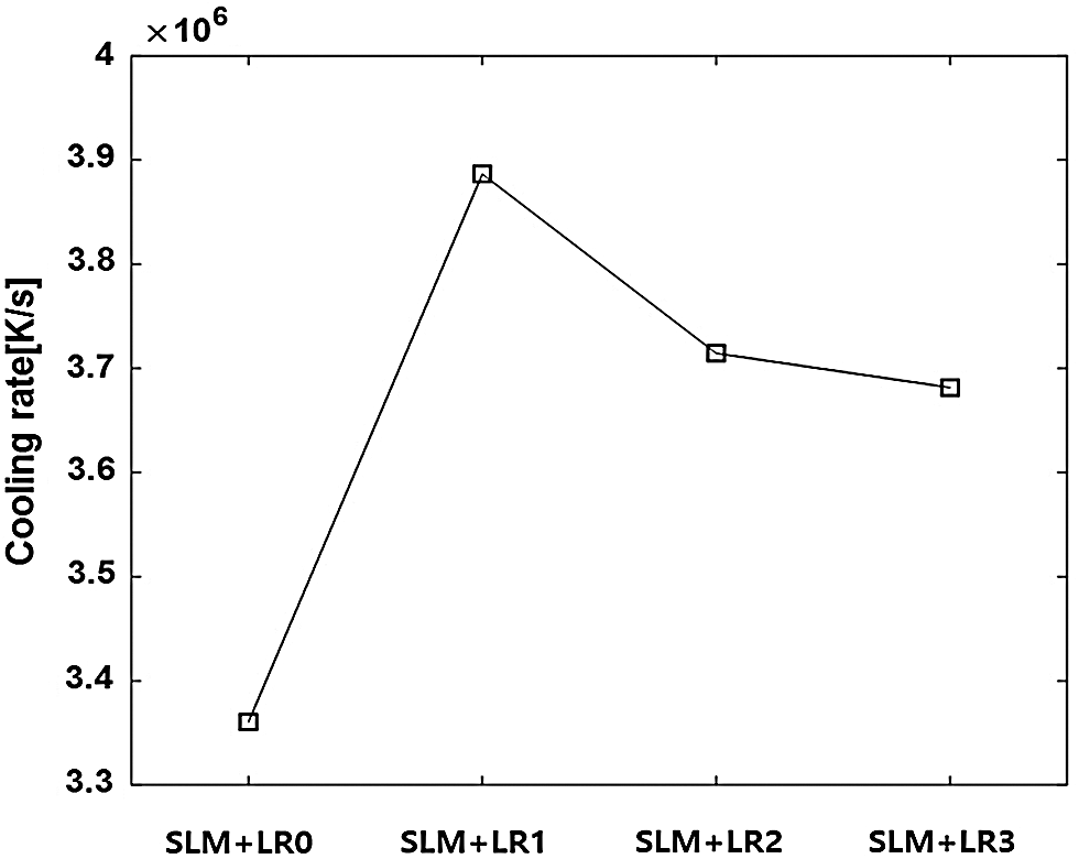
Figure 11: The observed maximum cooling rate after local solidification for different process conditions
Using the obtained temperature field from the thermal analysis, the stress field is obtained to investigate the effect of the re-melting process on the residual stress formation. Fig. 12 shows the Mises’ stress distribution after the temperature is cooled down to the ambient temperature 298 K. It is worth noting that there is a remarkable reduction in the stress level from SLM + LR1 to SLM + LR2 and a similar trend is observed in the cooling rate (Fig. 11). Fig. 13 shows the stress component S11 (where 11 is the scanning direction) which is the dominant stress component. The results show that the tensile residual stress is distributed on the top of the layer due to the shrinkage after the consolidation of the material. Figs. 14 and 15 show the stress component S22 (where 22 is the transverse direction) and the stress component S33 (where 33 is the build direction) respectively which are both smaller than the S11 component.
Figure 12: VonMises stress distribution with the different number of re-melting processes. a) SLM + LR0, b) SLM + LR1, c) SLM + LR2, d) SLM + LR3
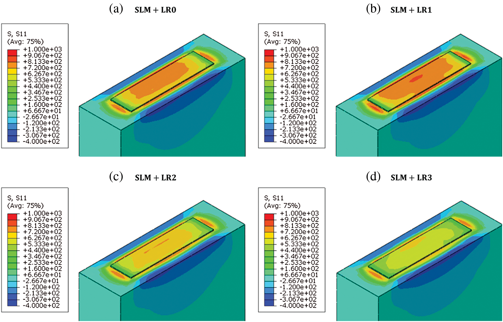
Figure 13: S11(scanning direction) distribution with the different number of re-melting processes. a) SLM + LR0, b) SLM + LR1, c) SLM + LR2, d) SLM + LR3
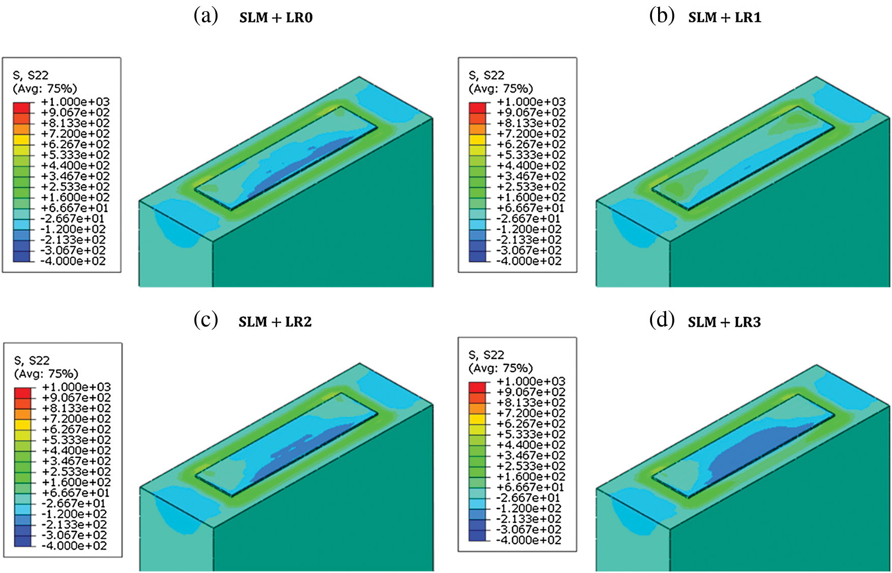
Figure 14: S22 distribution with the different number of re-melting processes. a) SLM + LR0, b) SLM + LR1, c) SLM + LR2, d) SLM + LR3
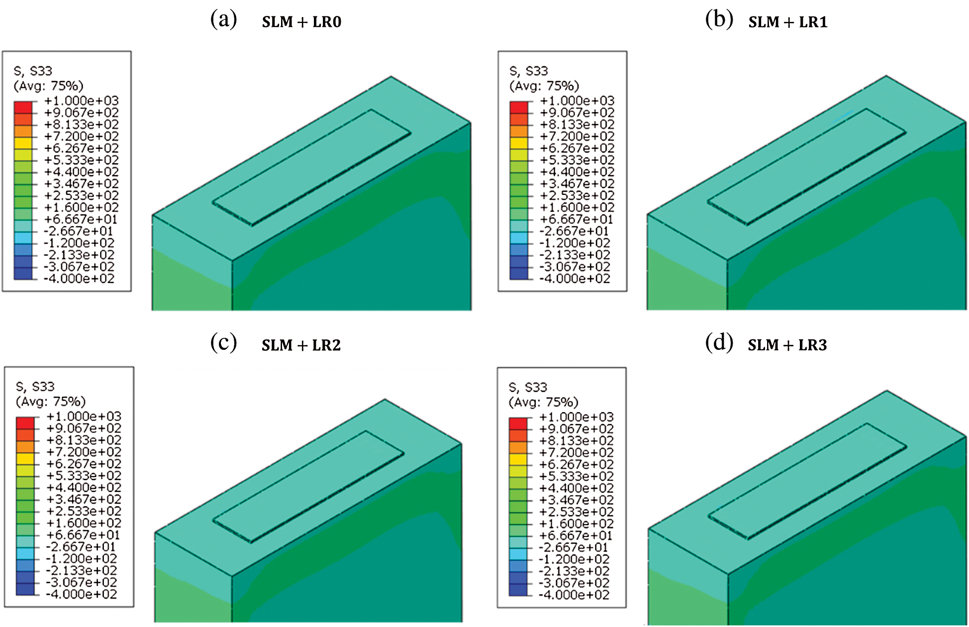
Figure 15: S33 distribution with the different number of re-melting processes. a) SLM + LR0, b) SLM + LR1, c) SLM + LR2, d) SLM + LR3
To investigate the effect of the re-melting process on the degree of the residual stress, the average values of Mises’ stress and S11 in the scanned layer are computed as shown in Fig. 16. The values of both the Mises’ stress and S11 show that they have a similar trend. After one re-melting process (SLM + LR1), the average Mises’ stress increases to 723 MPa as the cooling rate becomes higher than the case without the re-melting process (708 MPa). It is worth noting that the temperature gradient is more severe at the boundary between the melt pool and the powder material for the SLM + LR0 case as shown in Fig. 10a, but the overall stress level is lower than that of SLM + LR1 because the powder material is not activated (low stiffness). Then, the stress level significantly decreases to average Mises’ stress of 650 MPa in the SLM + LR2 case which is even lower than that of the SLM+LR0 case due to the accumulated heat in the layer. This trend is also in good agreement with the experimental measurement in the previous literature [18]. These analysis results show that the re-melting process should be applied with careful consideration of the phase change and the heat transfer mechanisms in the SLM process. It is also worthy to know that even though the cooling rate and the stress level showed a similar trend, the cooling rate with the re-melting processes always showed higher value compared to the case without re-melting (Fig. 11). This implies that the interpretation of results from the single thermal analysis may be insufficient to provide clues for the evaluation of the process. Thus, the parameter optimization and the process design with re-melting processes for SLM needs to be conducted considering both the thermal and mechanical approaches. In this regard, the proposed simulation framework and the modeling methods can support the quantitative and qualitative understandings of the SLM process.
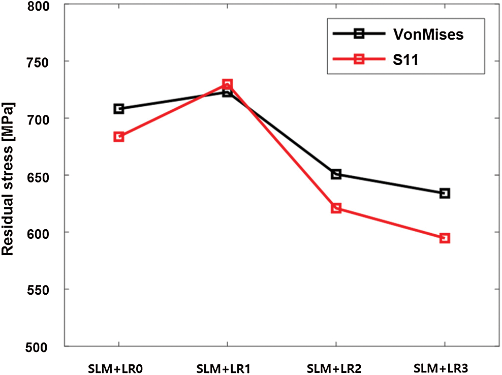
Figure 16: Average residual stress values in the single layer with the different number of re-melting processes
In this study, a thermo-mechanical analysis framework for SLM process simulation with the heat transfer model based on the phase-field approach, and the state-dependent thermal and mechanical material properties is proposed with the detailed implementation process. Using the introduced methodology, other thermo-dynamically consistent heat transfer models can be implemented in the commercial finite element tool ABAQUS. The heat transfer model is validated using the existing experimental data with varying laser power ( ) with the simulation of the SLM process with a single scan track. Furthermore, single layer scanning processes with multiple scan tracks and several re-melting processes are simulated to investigate the effect of re-melting on the temperature and the stress field. The results obtained conducting the thermo-mechanical analysis on the proposed framework are discussed and the important conclusions are:
1.The heat transfer model based on thermo-dynamically consistent phase-field approach is implemented successfully in ABAQUS/Standard using the user-subroutine and used in a thermo-mechanical simulation of the SLM process
2.The predicted melt pool dimension has a similar trend and good agreement with the experimental results, but the discrepancy becomes larger as the higher laser power is applied if the consolidation of the material and the vaporization is not considered.
3.From the simulation results of the single-track scanning process with varying laser powers (20–80 W), the minimum cooling rate is observed with the laser power of 80 W, and the maximum cooling rate is observed at the time after the local solidification with the laser power of  . Based on this result, the increase in laser power can help to mitigate the high-temperature gradient. However, the increase of the laser power leads to intense material vaporization which is not preferred in the SLM process.
4.The variation of the stress level with re-melting processes is investigated. The result shows that the stress level increases with one re-melting process, and decreases with the subsequent re-melting processes due to the different heat transfer mechanisms between the porous and dense material which is also in a good agreement with the experimental result.
5.The obtained maximum cooling rates for cases with a different number of re-melting processes show a similar trend with the variation of the stress level. However, the stress level decreases lower than that of the process without re-melting after two times of re-melting cycles whereas the cooling rate is higher for the case with the re-melting process.
Based on the proposed thermo-mechanical simulation framework, the SLM process can be evaluated considering various analysis results (melt pool dimensions, phase field, cooling rates, and residual stress field). For future work, simulation in a wider range of process windows will be investigated and the sensitivity analysis for different process parameters and the re-melting cycles will be conducted with extensive computations.
Funding Statement: This work was supported by the Korea Evaluation Institute of Industrial Technology (KEIT) grant funded by the Korea government (MOTIE, https://itech.keit.re.kr/index.do#00010000) (No. 20004662, Industrial Technology Innovation Program, Grantee: GJY) and Institute of Engineering Research (Grantee: GJY) at Seoul National University (https://www.snu.ac.kr/). The authors are grateful for their supports.
Conflicts of Interest: The authors declare that they have no conflicts of interest to report regarding the present study.
References
1. ASTM. (2012). “Standard terminology for additive manufacturing technologies,”.
2. D. Herzog, V. Seyda, E. Wycisk and C. Emmelmann. (2016). “Additive manufacturing of metals,” Acta Materialia, vol. 117, pp. 371–392.
3. C. Y. Yap, C. K. Chua, Z. L. Dong, Z. H. Liu, D. Q. Zhang et al. (2015). , “Review of selective laser melting: Materials and applications,” Applied Physics Reviews, vol. 2, no. 4, 041101.
4. M. Wong, S. Tsopanos, C. J. Sutcliffe and I. Owen. (2007). “Selective laser melting of heat transfer devices,” Rapid Prototyping Journal, vol. 13, no. 5, pp. 291–297.
5. P. Rochus, J. Y. Plesseria, M. Van Elsen, J. P. Kruth, R. Carrus et al. (2007). , “New applications of rapid prototyping and rapid manufacturing (RP/RM) technologies for space instrumentation,” Acta Astronautica, vol. 61, no. 1–6, pp. 352–359.
6. B. Vandenbroucke and J. P. Kruth. (2007). “Selective laser melting of biocompatible metals for rapid manufacturing of medical parts,” Rapid Prototyping Journal, vol. 13, no. 4, pp. 196–203.
7. A. T. Clare, P. R. Chalker, S. Davies, C. J. Sutcliffe and S. Tsopanos. (2008). “Selective laser melting of high aspect ratio 3D nickel-titanium structures two way trained for MEMS applications,” International Journal of Mechanics and Materials in Design, vol. 4, no. 2, pp. 181–187.
8. D. A. Hollander, M. Von Walter, T. Wirtz, R. Sellei, B. Schmidt-Rohlfing et al. (2006). , “Structural, mechanical and in vitro characterization of individually structured Ti-6Al–4V produced by direct laser forming,” Biomaterials, vol. 27, no. 7, pp. 955–963.
9. J. P. Kruth, G. Levy, F. Klocke and T. Childs. (2007). “Consolidation phenomena in laser and powder-bed based layered manufacturing,” CIRP Annals, vol. 56, no. 2, pp. 730–759.
10. D. Gu, Y. C. Hagedorn, W. Meiners, G. Meng, R. J. S. Batista et al. (2012). , “Densification behavior, microstructure evolution, and wear performance of selective laser melting processed commercially pure titanium,” Acta Materialia, vol. 60, no. 9, pp. 3849–3860.
11. R. Li, Y. Shi, Z. Wang, L. Wang, J. Liu et al. (2010). , “Densification behavior of gas and water atomized 316L stainless steel powder during selective laser melting,” Applied Surface Science, vol. 256, no. 13, pp. 4350–4356.
12. D. Karalekas and D. Rapti. (2002). “Investigation of the processing dependence of SL solidification residual stresses,” Rapid Prototyping Journal, vol. 8, no. 4, pp. 243–247.
13. P. Mercelis and J. P. Kruth. (2006). “Residual stresses in selective laser sintering and selective laser melting,” Rapid Prototyping Journal, vol. 12, no. 5, pp. 254–265.
14. R. Li, Y. Shi, Z. Wang, L. Wang, J. Liu et al. (2010). , “Densification behavior of gas and water atomized 316L stainless steel powder during selective laser melting,” Applied Surface Science, vol. 256, no. 13, pp. 4350–4356.
15. E. Yasa, J. Deckers and J. P. Kruth. (2011). “The investigation of the influence of laser re-melting on density, surface quality and microstructure of selective laser melting parts,” Rapid Prototyping Journal, vol. 17, no. 5, pp. 312–327.
16. M. Shiomi, K. Osakada, K. Nakamura, T. Yamashita and F. Abe. (2004). “Residual stress within metallic model made by selective laser melting process,” CIRP Annals, vol. 53, no. 1, pp. 195–198.
17. J. P. Kruth, J. Deckers, E. Yasa and R. Wauthlé. (2012). “Assessing and comparing influencing factors of residual stresses in selective laser melting using a novel analysis method,” in Proc. of the Institution of Mechanical Engineers, Part B: Journal of Engineering Manufacture, vol. 226, no. 6, pp. 980–991.
18. K. Wei, M. Lv, X. Zeng, Z. Xiao, G. Huang et al. (2019). , “Effect of laser remelting on deposition quality, residual stress, microstructure, and mechanical property of selective laser melting processed Ti-5Al-2.5 Sn alloy,” Materials Characterization, vol. 150, pp. 67–77.
19. H. Chen, Q. Wei, Y. Zhang, F. Chen, Y. Shi et al. (2019). , “Powder-spreading mechanisms in powder-bed-based additive manufacturing: Experiments and computational modeling,” Acta Materialia, vol. 179, pp. 158–171.
20. H. Chen, Q. Wei, S. Wen, Z. Li and Y. Shi. (2017). “Flow behavior of powder particles in layering process of selective laser melting: Numerical modeling and experimental verification based on discrete element method,” International Journal of Machine Tools and Manufacture, vol. 123, pp. 146–159.
21. S. A. Khairallah, A. T. Anderson, A. Rubenchik and W. E. King. (2016). “Laser powder-bed fusion additive manufacturing: Physics of complex melt flow and formation mechanisms of pores, spatter, and denudation zones,” Acta Materialia, vol. 108, pp. 36–45.
22. W. Yan, W. Ge, Y. Qian, S. Lin, B. Zhou et al. (2017). , “Multi-physics modeling of single/multiple-track defect mechanisms in electron beam selective melting,” Acta Materialia, vol. 134, pp. 324–333.
23. C. Fu and Y. Guo. (2014). “Three-dimensional temperature gradient mechanism in selective laser melting of Ti-6Al-4V,” Journal of Manufacturing Science and Engineering, vol. 136, no. 6, 061004.
24. A. Gusarov, I. Yadroitsev, P. Bertrand and I. Smurov. (2009). “Model of radiation and heat transfer in laser-powder interaction zone at selective laser melting,” Journal of Heat Transfer, vol. 131, no. 7, 072101.
25. A. Hussein, L. Hao, C. Yan and R. Everson. (2013). “Finite element simulation of the temperature and stress fields in single layers built without-support in selective laser melting,” Materials & Design (1980-2015), vol. 52, pp. 638–647.
26. L. Parry, I. Ashcroft and R. D. Wildman. (2016). “Understanding the effect of laser scan strategy on residual stress in selective laser melting through thermo-mechanical simulation,” Additive Manufacturing, vol. 12, pp. 1–15.
27. A. Foroozmehr, M. Badrossamay and E. Foroozmehr. (2016). “Finite element simulation of selective laser melting process considering optical penetration depth of laser in powder bed,” Materials & Design, vol. 89, pp. 255–263.
28. S. Roy, M. Juha, M. S. Shephard and A. M. Maniatty. (2018). “Heat transfer model and finite element formulation for simulation of selective laser melting,” Computational Mechanics, vol. 62, no. 3, pp. 273–284.
29. S. L. Wang, R. Sekerka, A. Wheeler, B. Murray, S. Coriell et al. (1993). , “Thermodynamically-consistent phase-field models for solidification,” Physica D: Nonlinear Phenomena, vol. 69, no. 1–2, pp. 189–200.
30. M. Boivineau, C. Cagran, D. Doytier, V. Eyraud, M. H. Nadal et al. (2006). , “Thermophysical properties of solid and liquid Ti-6Al-4V (TA6V) alloy,” International Journal of Thermophysics, vol. 27, no. 2, pp. 507–529.
31. A. Seifter, G. Pottlacher, H. Jäger, G. Groboth and E. Kaschnitz. (1998). “Measurements of thermophysical properties of solid and liquid Fe-Ni alloys,” Berichte Der Bunsengesellschaft Für Physikalische Chemie, vol. 102, no. 9, pp. 1266–1271.
32. K. C. Mills. (2002). Recommended Values of Thermophysical Properties for Selected Commercial Alloys. Woodhead Publishing, Cambridge, England.
33. M. Rombouts, L. Froyen, A. Gusarov, E. H. Bentefour and C. Glorieux. (2005). “Photopyroelectric measurement of thermal conductivity of metallic powders,” Journal of Applied Physics, vol. 97, no. 2, 024905.
34. Z. Fan and F. Liou. (2012). “Numerical modeling of the additive manufacturing (AM) processes of titanium alloy, ” in Titanium Alloys: Towards Achieving Enhanced Properties for Diversified Applications. Rijeka, Croatia: Intech, pp. 3–28.
35. F. Verhaeghe, T. Craeghs, J. Heulens and L. Pandelaers. (2009). “A pragmatic model for selective laser melting with evaporation,” Acta Materialia, vol. 57, no. 20, pp. 6006–6012.
36. G. Welsch, R. Boyer and E. Collings. (1993). Materials Properties Handbook: Titanium Alloys. OH, USA: ASM International.
37. M. Badrossamay and T. Childs. (2007). “Further studies in selective laser melting of stainless and tool steel powders,” International Journal of Machine Tools and Manufacture, vol. 47, no. 5, pp. 779–784.
38. S. Koric and B. G. Thomas. (2008). “Thermo-mechanical models of steel solidification based on two elastic visco-plastic constitutive laws,” Journal of Materials Processing Technology, vol. 197, no. 1–3, pp. 408–418.
39. I. A. Roberts, C. Wang, R. Esterlein, M. Stanford and D. Mynors. (2009). “A three-dimensional finite element analysis of the temperature field during laser melting of metal powders in additive layer manufacturing,” International Journal of Machine Tools and Manufacture, vol. 49, no. 12–13, pp. 916–923.
40. C. Van Gestel. (2015). “Study of physical phenomena of selective laser melting towards increased productivity,” EPFL.
41. E. Toyserkani, A. Khajepour and S. Corbin. (2004). “3-D finite element modeling of laser cladding by powder injection: Effects of laser pulse shaping on the process,” Optics Lasers in Engineering, vol. 41, no. 6, pp. 849–867.
42. K. Dai and L. Shaw. (2005). “Finite element analysis of the effect of volume shrinkage during laser densification,” Acta Materialia, vol. 53, no. 18, pp. 4743–4754.
43. P. Yuan and D. Gu. (2015). “Molten pool behaviour and its physical mechanism during selective laser melting of TiC/AlSi10Mg nanocomposites: Simulation and experiments,” Journal of Physics D: Applied Physics, vol. 48, no. 3, 035303.
44. L. Dong, A. Makradi, S. Ahzi and Y. Remond. (2009). “Three-dimensional transient finite element analysis of the selective laser sintering process,” Journal of Materials Processing Technology, vol. 209, no. 2, pp. 700–706.
45. R. B. Patil and V. Yadava. (2007). “Finite element analysis of temperature distribution in single metallic powder layer during metal laser sintering,” International Journal of Machine Tools Manufacture, vol. 47, no. 7–8, pp. 1069–1080.
46. Y. Shi, H. Shen, Z. Yao and J. Hu. (2007). “Temperature gradient mechanism in laser forming of thin plates,” Optics Laser Technology, vol. 39, no. 4, pp. 858–863.
47. I. A. Roberts. (2012). “Investigation of residual stresses in the laser melting of metal powders in additive layer manufacturing,”.
48. B. Cheng, S. Price, J. Lydon, K. Cooper and K. Chou. (2014). “On process temperature in powder-bed electron beam additive manufacturing: Model development and validation,” Journal of Manufacturing Science Engineering, vol. 136, no. 6, 061018.
49. B. Cheng and K. Chou. (2015). “Melt pool evolution study in selective laser melting,” in 26th Annual Int. Solid Freeform Fabrication Sym.–An Additive Manufacturing Conf., Austin, TX, USA, pp. 1182–1194.
50. M. J. Ansari, D. S. Nguyen and H. S. Park. (2019). “Investigation of SLM process in terms of temperature distribution and melting pool size: Modeling and experimental approaches,” Materials, vol. 12, no. 8, pp. 1272.
51. Y. Li and D. Gu. (2014). “Thermal behavior during selective laser melting of commercially pure titanium powder: Numerical simulation and experimental study,” Additive Manufacturing, vol. 1, pp. 99–109.
52. J. Goldak, A. Chakravarti and M. Bibby. (1984). “A new finite element model for welding heat sources,” Metallurgical Transactions B, vol. 15, no. 2, pp. 299–305.
53. J. Xie, V. Oancea and J. Hurtado. (2017). “Phase transformations in metals during additive manufacturing processes,” in NAFEMS World Cong., Stockholm.
54. C. Bruna-Rosso, A. G. Demir and B. Previtali. (2018). “Selective laser melting finite element modeling: Validation with high-speed imaging and lack of fusion defects prediction,” Materials & Design, vol. 156, pp. 143–153.
55. P. Rangaswamy, M. B. Prime, M. Daymond, M. Bourke, B. Clausen et al. (1999). , “Comparison of residual strains measured by X-ray and neutron diffraction in a titanium (Ti-6Al–4V) matrix composite,” Materials Science Engineering: A, vol. 259, no. 2, pp. 209–219.
56. M. Fukuhara and A. Sanpei. (1993). “Elastic moduli and internal frictions of Inconel 718 and Ti-6Al-4V as a function of temperature,” Journal of Materials Science Letters, vol. 12, no. 14, pp. 1122–1124.
57. M. Vanderhasten, L. Rabet and B. Verlinden. (2008). “Ti-6Al–4V: Deformation map and modelisation of tensile behaviour,” Materials Design, vol. 29, no. 6, pp. 1090–1098.
58. P. Rangaswamy, H. Choo, M. B. Prime, M. A. Bourke and J. M. Larsen. (2000). “High temperature stress assessment in SCS-6/TI-6A1-4V composite using neutron diffraction and finite element modeling,” in Int. Conf. on Processing & Manufacturing of Advanced Materials, Las Vegas, NV, USA.
59. ABAQUS. (2016). Theory Manual: Dassault Systms.
60. D. Systèmes. (2010). “Abaqus 6.10 online documentation,” Abaqus User Subroutines Reference Manual.
61. A. Faghri, Y. Zhang and J. R. Howell. (2010). Advanced Heat and Mass Transfer. Global Digital Press, Columbia, MO, USA.
62. Q. Zhang, J. Xie, Z. Gao, T. London, D. Griffiths et al. (2019). , “A metallurgical phase transformation framework applied to SLM additive manufacturing processes,” Materials & Design, vol. 166, pp. 107618.
63. W. E. King, H. D. Barth, V. M. Castillo, G. F. Gallegos, J. W. Gibbs et al. (2014). , “Observation of keyhole-mode laser melting in laser powder-bed fusion additive manufacturing,” Journal of Materials Processing Technology, vol. 214, no. 12, pp. 2915–2925.
64. A. Bauereiß, T. Scharowsky and C. Körner. (2014). “Defect generation and propagation mechanism during additive manufacturing by selective beam melting,” Journal of Materials Processing Technology, vol. 214, no. 11, pp. 2522–2528.
65. J. Dilip, S. Zhang, C. Teng, K. Zeng, C. Robinson et al. (2017). , “Influence of processing parameters on the evolution of melt pool, porosity, and microstructures in Ti-6Al-4V alloy parts fabricated by selective laser melting,” Progress in Additive Manufacturing, vol. 2, no. 3, pp. 157–167.
66. J. Trapp, A. M. Rubenchik, G. Guss and M. J. Matthews. (2017). “In situ absorptivity measurements of metallic powders during laser powder-bed fusion additive manufacturing,” Applied Materials Today, vol. 9, pp. 341–349.
67. D. R. Askeland, P. P. Fulay and W. J. Wright. (2011). The Science and Engineering of Materials. Stamford, CT, USA.
68. Z. Hu, H. Zhu, C. Zhang, H. Zhang, T. Qi et al. (2018). , “Contact angle evolution during selective laser melting,” Materials Design, vol. 139, pp. 304–313.
69. W. E. King, A. T. Anderson, R. M. Ferencz, N. E. Hodge, C. Kamath et al. (2015). , “Laser powder bed fusion additive manufacturing of metals; physics, computational, and materials challenges,” Applied Physics Reviews, vol. 2, no. 4, 041304.
70. C. Chen, J. Yin, H. Zhu, Z. Xiao, L. Zhang et al. (2019). , “Effect of overlap rate and pattern on residual stress in selective laser melting,” International Journal of Machine Tools Manufacture, vol. 145, 103433.
 | This work is licensed under a Creative Commons Attribution 4.0 International License, which permits unrestricted use, distribution, and reproduction in any medium, provided the original work is properly cited. |