SW-Net: A novel few-shot learning approach for disease subtype prediction

Introduction

Disease sub-type prediction aims at identifying sub-types of patients so that it permits a more accurate assessment of prognosis (Saria and Goldenberg, 2015). Predicting disease sub-types with gene expression data is of great significance in molecular biology (Rukhsar et al., 2022). Accurate classification allows a more efficient and targeted succeeding therapy (Sohn et al., 2017). However, patient genomic data are hard to deal with because of the “big p, small N” issue, which means high dimensional features with a small number of samples (Liang et al., 2013). Especially when the disease is rare (Yoo et al., 2021), this is a very crucial problem faced by doctors and clinicians. Few-shot learning, which aims at dealing with the “small data” issue, has attracted lots of attention, and researchers have made significant progress in many fields, such as computer vision (Li et al., 2006; Munkhdalai and Yu, 2017; Snell et al., 2017; Qiu et al., 2018; Mishra et al., 2018; Sung et al., 2018). Recently, researchers have explored few-shot learning methods for genomic data and achieved good performance in genomic survival analysis (Qiu et al., 2020). This motivates us to introduce few-shot learning for genomic analysis. Our goal in this study was to address the issue of the few-shot disease sub-type prediction problem. This problem is considered in isolation in traditional machine learning methods. However, in practice, doctors and clinicians take several clinical factors into account simultaneously.

The basic idea of our proposed new model was to learn from relevant abundant tasks and generalize to new classes, which are rare diseases. This mimics the process by which doctors and clinicians study the prediction of disease sub-types. The model extracts shared knowledge or experience from a range of interrelated tasks and applies it to new tasks. Although increasingly complex models are being proposed, experiments show that a simple baseline approach can achieve desired results comparable to other complex methods. The training procedure of our model includes a pre-training stage and a fine-tuning stage, which is similar to the transfer learning procedure (Weiss et al., 2016). In the first stage, we trained a feature extractor and a classifier at the same time with the base classes. In the fine-tuning stage, we fixed the parameters of the feature extractor. However, a new classifier is learned in this stage with the few samples with tags in the new class. In fact, with some twists of performing fine-tuning and regularization, a simple baseline method outperforms many other competing algorithms on few-shot sub-type prediction tasks.

Most few-shot models are originally designed for images (Vinyals et al., 2016; Finn et al., 2017; Garcia and Bruna, 2017; Bertinetto et al., 2018; Rusu et al., 2018; Lee et al., 2019). However, the high dimensionality of genomic data makes predictions more difficult compared to images because of the large number of redundant features. To address this issue, our new model appends a feature selection module, which is first proposed by Yang et al. (2020) to solve the dimensionality issues.

High noise is another challenging topic for accurate sub-type prediction. Random noise and system bias may be prone to overfitting and affect performance in generalization (Liang et al., 2013). Commonly weights are assigned to samples to deal with this issue. Opinions vary on the relationship between sample weight and training loss: one holds that the samples with larger training loss should be more emphasized since they are more likely to be complex ones that are located at the classification boundary. Typical methods include AdaBoost (Freund and Schapire, 1997) and focal loss (Lin et al., 2020). On the contrary, another approach is to give priority to samples with smaller losses because these are more likely to have high confidence. Typical methods include self-paced learning (Kumar et al., 2010), iterative reweighting (de la Torre and Black, 2003) and its variants (Jiang et al., 2014; Wang et al., 2017). Meta-weight-net (Shu et al., 2019) designed a network that adaptively learns an explicit weighting function directly from data. This methodology prioritizes small loss samples and is especially suitable for heavy noise scenarios. The rationality lies in that the samples with large losses may possibly have corrupted labels, and the reweighting approach could suppress this issue to a certain degree. Since high noise is a vital problem in gene expression data, we adopted the method of Shu et al. (2019) to assign weight to the samples and give higher weight to the data with low loss to suppress the influence of the samples with high noise.

In summary, the proposed SW-Net mainly made the following contributions.

First, we applied a new baseline method in the few-shot disease sub-type prediction problem. The basic baseline has been widely explored in many fields, especially computer vision. Our contribution is to modify this baseline method in the field of molecular biology, especially for disease subtype prediction problems. The new model fits well. We used support-based initialization for the classifier and transductive fine-tuning technique in our work. We also append an entropy regularization term on the query set to reduce overfitting.

Second, based on the baseline, we further extended a feature selection module and a sample weighting module to solve the high dimensionality issue for few-shot prediction. The extended modules aim to adaptively select vital features and give priority to samples with small losses.

Third, experiments show that with support-based initialization and transductive fine-tuning, we can achieve a 2%–6% improvement in prediction accuracy. With the appended feature selection and sample weighting modules, we can further achieve a 2%–2.5% improvement on The Cancer Genome Atlas (TCGA) meta-dataset.

Materials and Methods

In this part, we first show the basic baseline model for few-shot learning. Then, we present the variants we performed to improve its performance. Finally, we elaborate our extended modules. The model architecture is shown in Fig. 1.

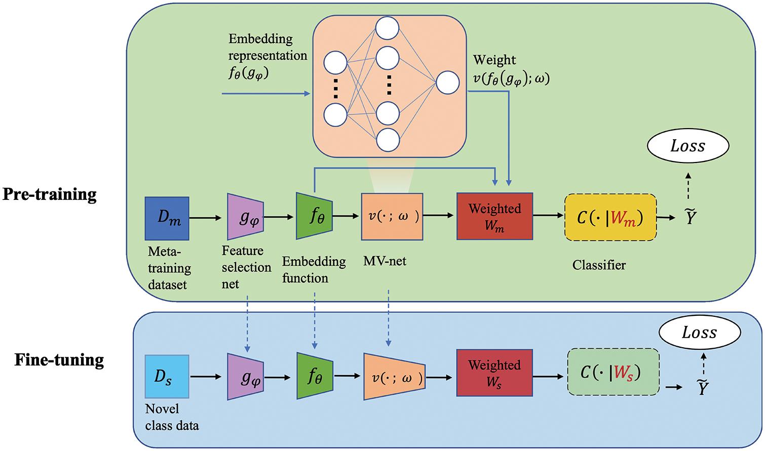
Figure 1: Structure of SW-Net. We trained a feature selector gφ, an embedding function fθ and a weighting function v with the meta-training dataset in the pre-training stage. In the fine-tuning stage, we train a new classifier C(·|Ws) with the samples with label in the support set. All the parameters are fine-tuned transductively.

Problem definition

To formalize the few-shot prediction problem, we need to introduce some notation first. Let (x,y) represent a labeled sample and its ground-truth label respectively. In the few-shot learning context, we let Ds={(xi,yi)}i=1Ns and Dq={(xi,yi)}i=1Nq denote the support and query datasets respectively. yi∈Ct represents some set of classes. The number of classes | Ct | is called the ways. The number of labeled samples in each class is called a shot. The goal is to train a network F to exploit the support set Ds to make a prediction of the label from the query set, by the following formula:

y^=F(x;Ds) (1)

where (xi,yi)∈Dq . A few-shot learning problem also has a meta-training dataset Dm={(xi,yi)}i=1Nm , with abundant data, where yi∈Cm . The set of classes Cm has no overlapping class with Ct . We can take advantage of Dm to give parameters of the learning model a good initialization.

Baseline

A simple baseline form includes the following steps: pre-training on the meta-training dataset, fine-tuning on the few-shot dataset and making few-shot predictions (Weiss et al., 2016; Chen et al., 2019). Our SW-Net follows the basic procedure. In the pre-training stage, we first trained a model with the cross-entropy loss on Dm={(xi,yi)}i=1Nm . With the training samples in meta-training set classes x∈Dm , we can learn a classifier C and an embedding function f that can transfer high dimensional data of a sample to the low dimensional feature vector. The feature vector will be used in the next stage. Fine-tuning stage: To make our model well-adapt to new classes, we fixed the network parameter θ in the embedding function fθ (called the backbone) from the pre-training stage, and then learn a new classifier C(⋅|Ws) , where Ws ∈ Rd∗Ct is the weight matrix, d represents the dimension of the feature vector, and Ct is the number of output classes. Ws is optimized by minimizing cross-entropy loss L with the few samples of support set. The classifier C(⋅|Ws) is a softmax classifier, which is built up with a linear layer and a softmax function as shown in Eq. (2):

Softmax(WsTfθ(xi)+b) (2)

Careful initialization of the softmax classifier C(⋅|Ws) will make this process efficient. We initialized this classifier with the feature mean of the support set to make it adapts well.

Making few-shot predictions: In this stage, given a query sample, fθ obtains the feature vector of the query sample. Then we entered it into the softmax classifier to make the final prediction.

Support based initialization

In a few-shot task, let Sc denote the samples in class c of the support set Ds . For the classifier, the weight and bias are Ws ∈ Rd∗Ct and b ∈ RCt , respectively, Ws=[w1,w2,…,wc,…] , where Ct denote the number of classes of Ds and each class of Ds is a d -dimensional vector. The first modification we perform is to initialize wc by the average feature of class c .

wc=1|Sc|∑x∈Sc⁡fθ(x) (3)

Intuitively, we can understand the weight vector Ws as a prototype, similar to (Snell et al., 2017). The classification is distance-based on the input feature and the prototypes, as shown in Fig. 2. Moreover, we initialized the bias bc=0 . Given the labeled samples of support set, we further fine-tune Ws , b , and θ by minimizing cross-entropy classification loss.

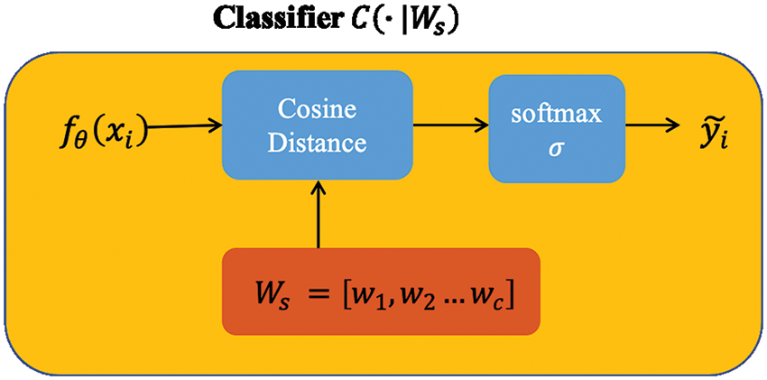
Figure 2: Vector Ws was initialized with the feature mean of each class. For each class, we computed the cosine distances between the input feature vector and the prototype weight vector.

Cosine distance-based classifier

We design the classifier here differently from the linear one used in the basic baseline to improve performance. According to Chen et al. (2019), the authors compared the effect of Euclidean distance and cosine distance on image datasets and found that cosine distance achieves better performance because of its reduced intra-class variation. For an input feature vector fθ(xi) , we compute its cosine distance to each weight vector Ws=[w1,w2,…,wc,…] . A prediction is made according to the probability that x is in class c with Eq. (4). Operator sim(,) denotes the cosine similarity between the input vectors and the weight vector.

p(y=c|x)=exp(sim(fθ(x),wc)∑c′⁡exp(sim(fθ(x),wc) (4)

Transductive fine-tuning

The main idea of transductive learning is to restrict hypothesis space with samples from the test dataset. Some papers in the few-shot learning field have exploited the idea of transductive learning recently. For example, Nichol et al. (2018) adapted batch-normalization parameters to query samples. Liu et al. (2018) estimated labels of query samples with label propagation. We denote Θ={θ,Ws,b} the combined parameters of fθ and C . All the parameters Θ are trained together in the fine-tuning stage.

At test time, we added a Shannon Entropy penalty term of query sample predictions. This is inspired by semi-supervised learning literature, close to work of Grandvalet and Bengio (2004). More recent methods like Dai et al. (2017) and Kipf and Welling (2016) are also suitable for our model, but we used the Shannon Entropy penalty for simplicity. We used unlabeled query samples for transductive learning. x represents a query sample. pΘ(⋅|x) is the prediction. H(pΘ(⋅|x)) stands for the Entropy. Multiple query samples can be processed together to get the mean of H(pΘ(⋅|x)) of all query samples, and we minimized cross-entropy classification loss over all query labels. As we seek outputs with a small Shannon Entropy H , we introduced the regularizer. Thus, the transductive fine-tuning learning for

Θ∗=arg⁡minΘ1Ns∑(x,y)∈Ds−log⁡pΘ(y|x)+1Nq∑(x,y)∈Dq⁡H(pΘ(⋅|x)) (5)

It is worth noting that the first term uses the samples with labels from the support set Ds , whereas the second term, which is the regularizer, utilizes the unlabeled samples from the query set Dq . The two terms can be imbalanced. We could add a coefficient for the entropy term to control the imbalance problem. However, we set it equal to 1 as we wish to keep its simplicity and avoid optimizing these hyper-parameters.

Feature selection net

We aimed to solve the few-shot disease sub-type prediction problem. However, genomic data is hard to handle due to the high dimensionality, as we mentioned above. To overcome this issue, we extend our baseline with a feature selection module to screen out the genes that are irrelevant to the disease. For each sample x∈Rp . The dimension of genomic data p can be very high. We can utilize a selection β = (β1, β2, …, βp). vector to get a new representation x′ which is the element-wise product of x′ and β . This can help us remove useless features.

x′=β⊙x,βj∈[0,1] (6)

Most regularization methods are based on some assumptions about the training data. However, when we do not have a significant understanding of the basics of gene expression data, it was not feasible to specify a specific regularization form. Here, we set a Softmax layer as the feature selection vector β . Then we obtained the element-wise product that can adaptively learn feature weighting from data.

x′=gφ(x)=β(φ)⊙xβi(φ)=exp(φ)i/∑jexp (φ)j,∑iβi(φ)=1(7)

where φ∈Rp represent the parameter of the Softmax classifier. Here we can easily embed gφ(x) into Eq. (4) and get:

pφ,θ(y=c|x)=exp(sim(fθ(gφ(x)),wc))∑c′⁡exp(sim(fθ(gφ(x)),wc′)) (8)

And in Eq. (3) becomes

wc=1|sc|∑x∈Sc⁡fθ(gφ(x)) (9)

This regularization form needs no expert knowledge of the underlying data. φ can be learned along with Θ . Now we donate the new combined parameters as Θ′={θ,Ws,b,φ}. All the parameters Θ′ are trained in the fine-tuning stage transductively:

(Θ′)∗=argminΘ1Ns∑(x,y)∈Ds−log⁡pΘ′(y|x)+1Nq∑(x,y)∈Dq⁡H(pΘ′(⋅|x)) (10)

Sample weighting net

The high noise issue in genomic data is another challenging problem. We set weights to samples to prioritize high-confidence data, with the hope to restrain the influence of the samples with high noise. The weight vector wc is the weighted representation of all samples for class c from the support set,

wc=1|sc|∑xi∈Sc⁡vi⋅fθ(gφ(xi)) (11)

where vi reflects how much we believe that sample xi is clean data. Larger weight vi represents we treat it as clean data with higher confidence.

To determine the v , we modified the method proposed by Shu et al. (2019), which attempts to learn a weighting function to assign different weights to clean the noisy samples. The sample weight v is an MLP network. The input of the MLP network is the loss for the sample, and the output of it is the weight, as shown in Fig. 1. Since our baseline model treats the support samples as prototypes and we did not compute the losses. The feature vector of each sample is the input instead of the loss. So, the Eq. (11) function can be rewritten as:

wc=1|sc|∑xi∈Sc⁡V(fθ(gφ(xi))ω)⋅fθ(gφ(xi)) (12)

Results

To evaluate the performance of our proposed SW-Net, we conducted experiments on both simulated data and the TCGA gene expression dataset. Our SW-Net outperformed conventional machine learning methods and typical few-shot methods.

Simulated dataset

We constructed the training dataset Dtrain and test dataset Dtest , where they had non-overlapping classes. We referred to the work of Ma and Zhang (2019) to generate simulated data. For Dtrain , we sampled 100 points from each of the ten Gaussian distributions, which were 2-dimensional distributions with covariance matrix and ten different mean μ = (2, 2), (6, 6), (0, −5), (4, −4), (−2, 2), (−5, 0), (−6, 6), (−2, −9), (−5, −5), (−9, −6), respectively as the true features. We then appended 40-dimensional Gaussian irrelevant features with the covariance matrix ∑=diag (10, …, 10) and mean μ = diag (2.5, …, 2.5). Therefore, each sample has 42-dimensional features, including the two true features and the forty irrelevant features. For Dtest , 1000 points were drawn from each of the four Gaussian distributions with the covariance matrix ∑=diag(1,1) and four different means μ = (0, 0), (1, 0), (0, 1), (1, 1), as the true features. Then we appended the 40-dimensional Gaussian irrelevant features the same as the setting.

Implementation details

We compared SW-Net with conventional machine learning methods and two typical meta-learning methods (including Prototypical net and Matching net). SW-Net was firstly pre-trained with the training dataset Dtrain , which contains 10 classes. Then we randomly selected 1% of the samples from Dtest , for each of the four classes as support datasets, and the remaining samples were placed into the query set. The accuracy of SW-Net was tested with 50 random runs. The conventional machine learning methods were trained on 1% of the test set per-class and tested on the remaining samples. The implementation detail adopts the same setting as the work in Ma and Zhang (2019).

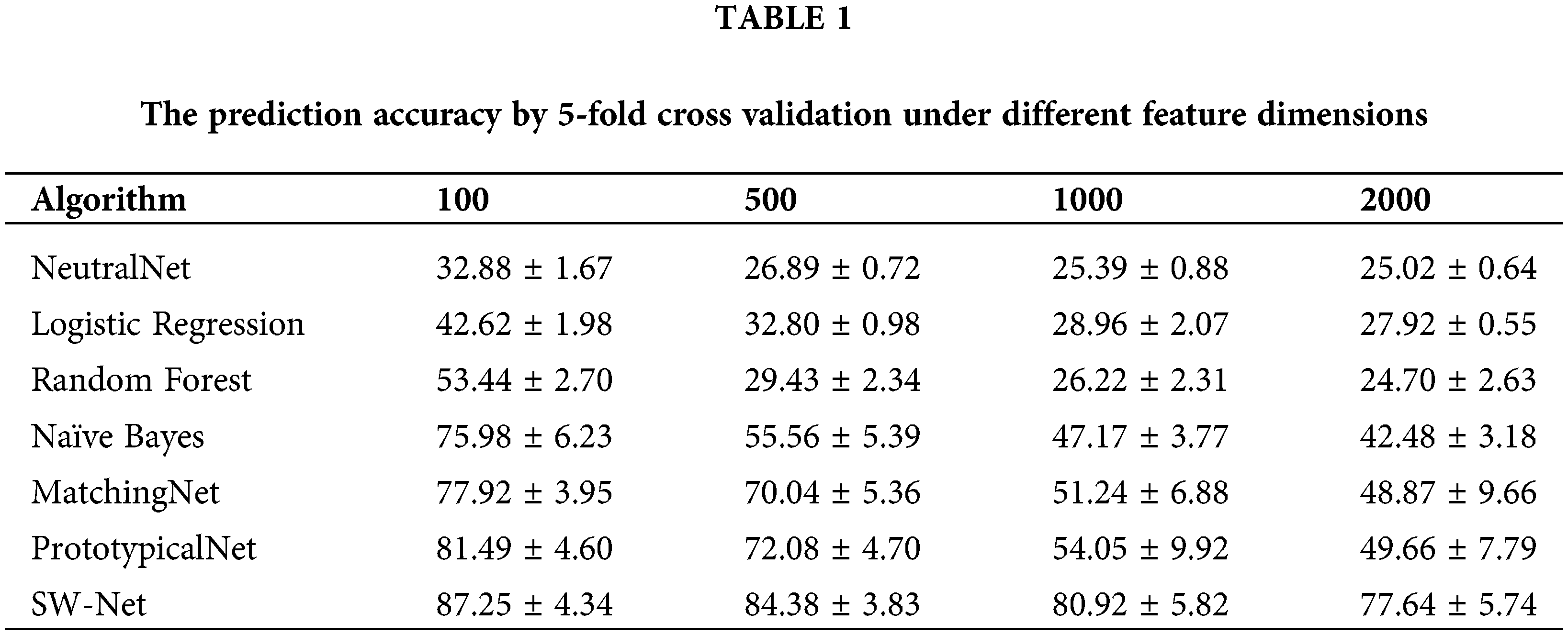
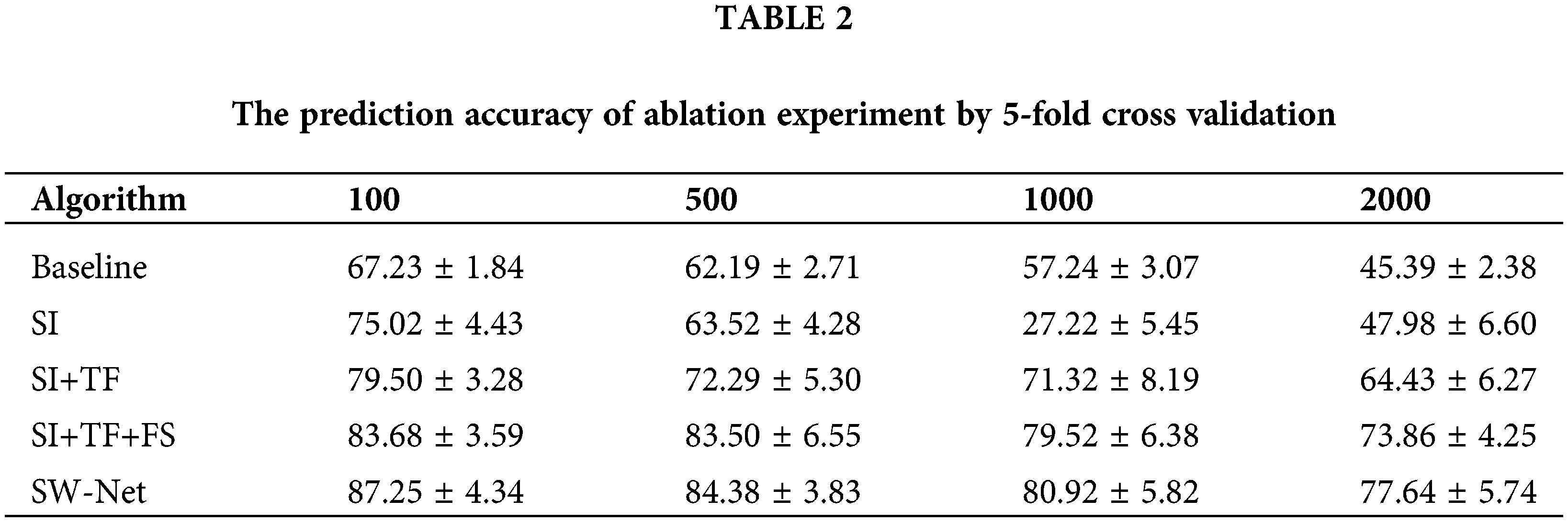
Results on different feature dimension settings

To test the feature selection capability of SW-Net, we increased irrelevant feature dimensions to four levels, which are 100, 500, 1000, and 2000, respectively. Basic implementation settings keep the same. The result is demonstrated in Tables 1 and 2 with 50 random runs by 5-fold cross-validation. In the ablation experiment, the baseline denotes the basic baseline model without any modifications. SI denotes “Support-based Initialization”; “SI+TF” means that Support-based Initialization and Transductive Fine-tuning were both added to the baseline; In “SI+TF+FS”, the FS denotes the Feature Selection net, and in SW-net, we added all modules, including the sample reweighting net, to the baseline. SW-Net outperformed all other comparison methods, including two typical meta-learning methods and five conventional machine-learning methods. With the increase of dimension, the performance gaps between SW-Net and the competing methods increased. This shows the capability of our model to deal with high-dimension data.

Moreover, we tested SW-Net’s ability to select vital features. We selected a representative machine learning method, which is Logistic Regression, and compared its learned weights of features with SW-Net on a 42-dimensional feature setting. Fig. 3 shows the learned weights of features by logistic regression, and Fig. 4 represents the weights of features learned by SW-Net; we can see that the red bar of SW-Net is much higher than the blue bar, which demonstrates that the selection of true features is better through our model compared with the conventional method.

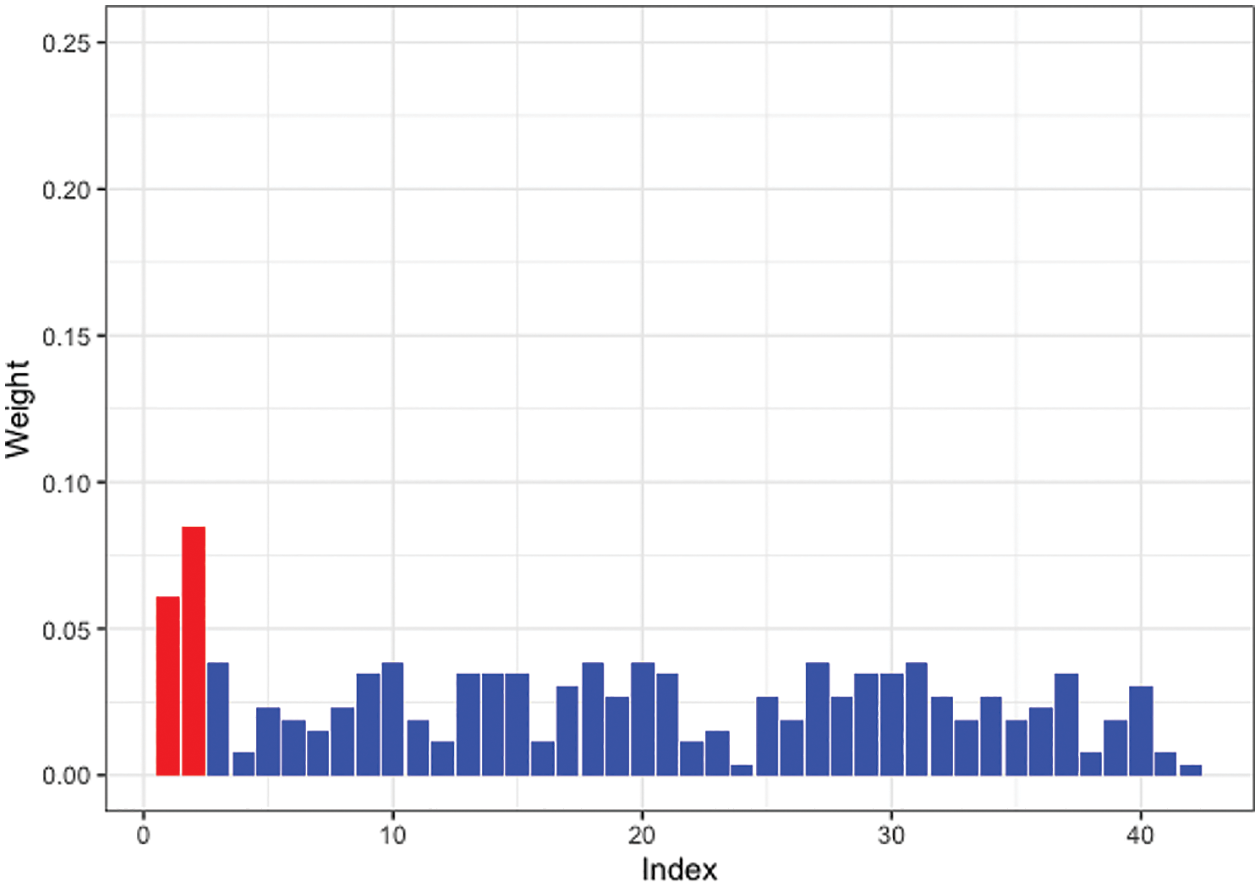
Figure 3: Learned feature weights by logistic regression on a simulated dataset. The red bar shows the true features.

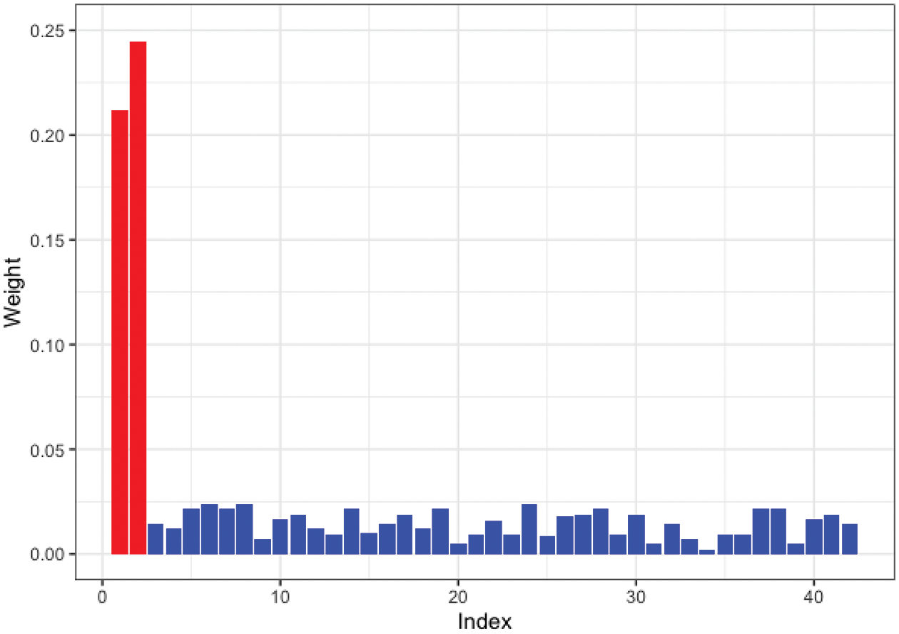
Figure 4: Learned feature weights by SW-Net on a simulated dataset. The red bar shows the true features.

Experiments on the cancer genome atlas meta-dataset

TCGA Meta-Dataset: The field of genomics lacks a consistent benchmark data set. To address this issue, TCGA Meta-Dataset (Samiei et al., 2019) offers a dataset from the publicly available clinical dataset, which is TCGA Program. There are 174 tasks which are all classification problems. The input gene-expression data is with 20530 genes. These are good proxy tasks to develop algorithms for few-shot problems. They consist of a variety of clinical problems, such as predicting tumor tissue site, histological type, and many others. The task definition and data can be found at https://github.com/mandanasmi/TCGA_Benchmark.

Implementation Details: We selected 68 clinical tasks from it. Each task included two classes and each class had no less than 60 samples. To evaluate the performance of SW-Net and other competing methods, we used 80 classes for training and tested the remaining 56 classes. They were tested on the 5-shot and 1-shot settings, respectively. For simplicity, we did not perform a separate hyper-parameter search. All methods utilized the same network as the backbone, which consisted of 2 fully connected layers, both with ReLU (Nair and Hinton, 2010) activation. The sizes of the two hidden layers were 6000 and 2000, and the output size was 200. We used the Adam optimizer, and the learning rates were determined based on a grid search of [0.001, 0.0005, 0.0001, 0.00005, 0.00001]. A learning rate of 0.0001 was selected for the pre-training stage. All other methods used the same learning rate of 0.0001. For the fine-tuning stage, an SGD optimizer with a 0.001 learning rate was selected.

We kept the backbone the same for all methods. For the conventional methods, we used the implementation in scikit-learn (https://scikit-learn.org/) for Naive Bayes, Logistic Regression, and Random Forest with default settings. We implemented NeuralNet and AffinityNet with default settings in the original paper (Ma and Zhang, 2019). For matching net, prototypical network, and the baseline method, we followed the implementation by Chen et al. (2019), https://github.com/wyharveychen/CloserLookFewShot. The selected tasks for our experiment can be found at https://drive.google.com/file/d/1cYzuMJKbxWsIZqbwhH1LW0bzfkW_Cc9h/view?usp=sharing.

Results on the cancer genome atlas meta-dataset

We compared SW-Net against the following methods: two representative meta-learning algorithms (including Matching Net and Prototypical Networks) and conventional learning methods (including Logistic Regression, Neural Network, and majority class prediction). We also conducted an ablation experiment to test the performance of each component of the proposed model. For the conventional methods, we randomly selected 120 samples for each task to take 80 of them as training data and use the rest for testing. Each task had two classes. For meta-learning methods and SW-Net, we tested them under 5-shot and 1-shot settings. The result is shown in Table 3. The query shot was set to 15 in this experiment unless otherwise specified. Fine-tuning was performed on one GPU for 30 epochs for SW-Net. Two updates for the weight were made in each epoch: we first updated the cross-entropy term with the support samples and then updated the Shannon Entropy term with the query samples.

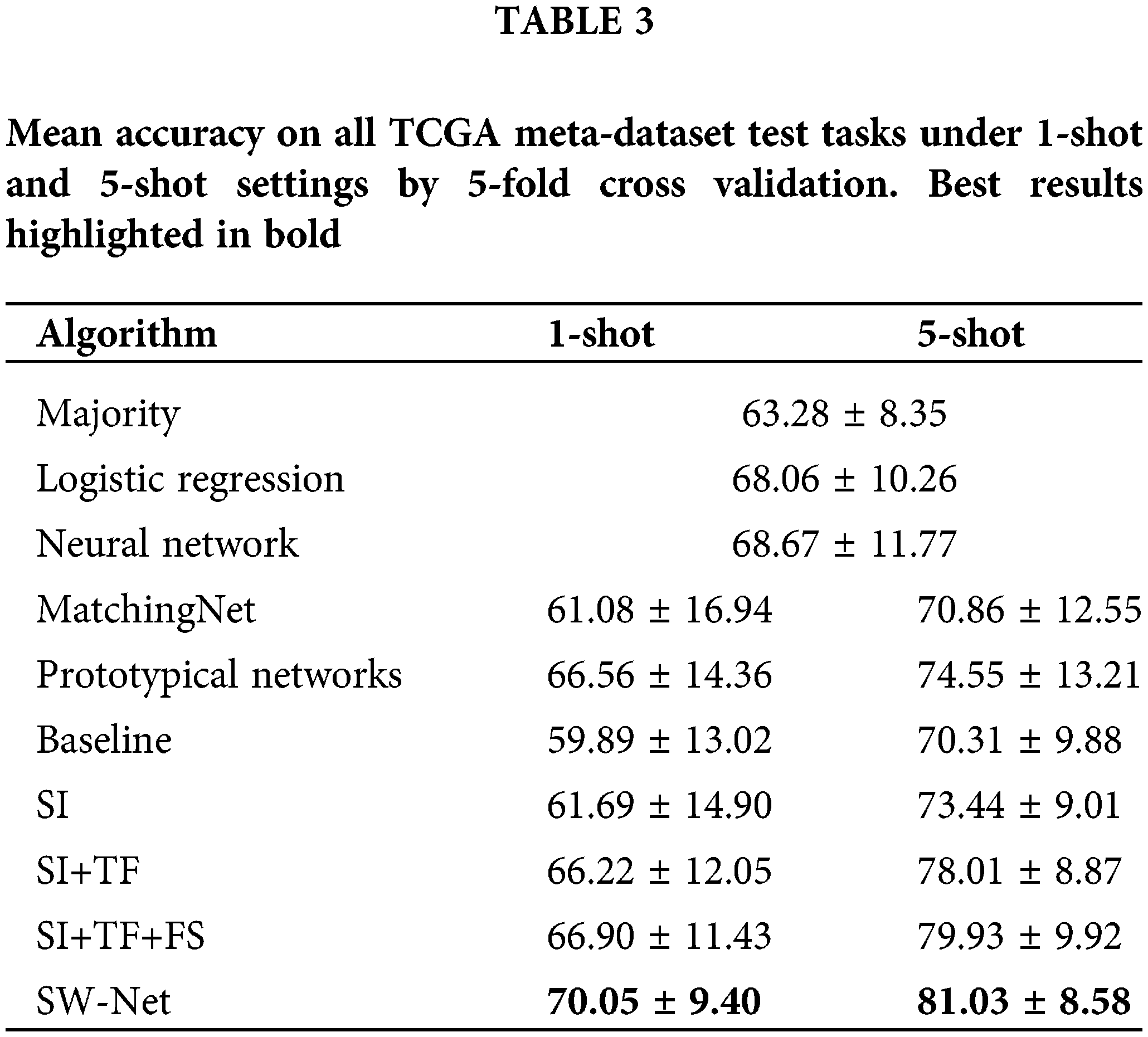
As in Table 3, the ablation experiment is mentioned in the bottom section of the table. If we only adopted support-based initialization, the performance can be comparable to the other meta-learning algorithms. For the 1-shot experiment, only performing support-based initialization leads to a minor improvement in accuracy over other methods. For the 5-shot setting, performing support-based initialization and fine-tuning obtains a better result than the other methods.

Transductive fine-tuning in the experiment results in a nearly 5% improvement in prediction accuracy for 1-shot over the support-based initialization. Meanwhile, it led to an improvement of nearly 4% prediction accuracy for the 5-shot setting. This demonstrates that the unlabeled query samples used in the transductive fine-tuning are vital for the few-shot setting. SW-Net led to 1%–2% improvement in 1-shot and 5-shot settings over transductive fine-tuning. This shows that the selection vector indeed filtered out the useless features and has a positive effect on the prediction accuracy.

We further compared SW-Net with other methods on the lung cancer subtype task and GBM (glioblastoma multiforme) gene expression subtype task separately under 5-shot settings through 5-fold cross-validation. The evaluation criterion included accuracy and area under the ROC curve (AUC). The result of accuracy is shown in Tables 4 and 5. “SI” denotes “Support-based Initialization”; “SI+TF” denotes “Support-based Initialization and transductive fine-tuning”; “SI+TF+FS” represents Feature Selection net is added; SW-net represents that we add the sample reweighting net to the previous model. In Fig. 5, we show the AUC on the lung cancer subtype task and GBM gene expression subtype task. The supported-based initialization improved both AUC and accuracy. Both tasks benefited from the feature selection module and sample reweighting module at different degrees.

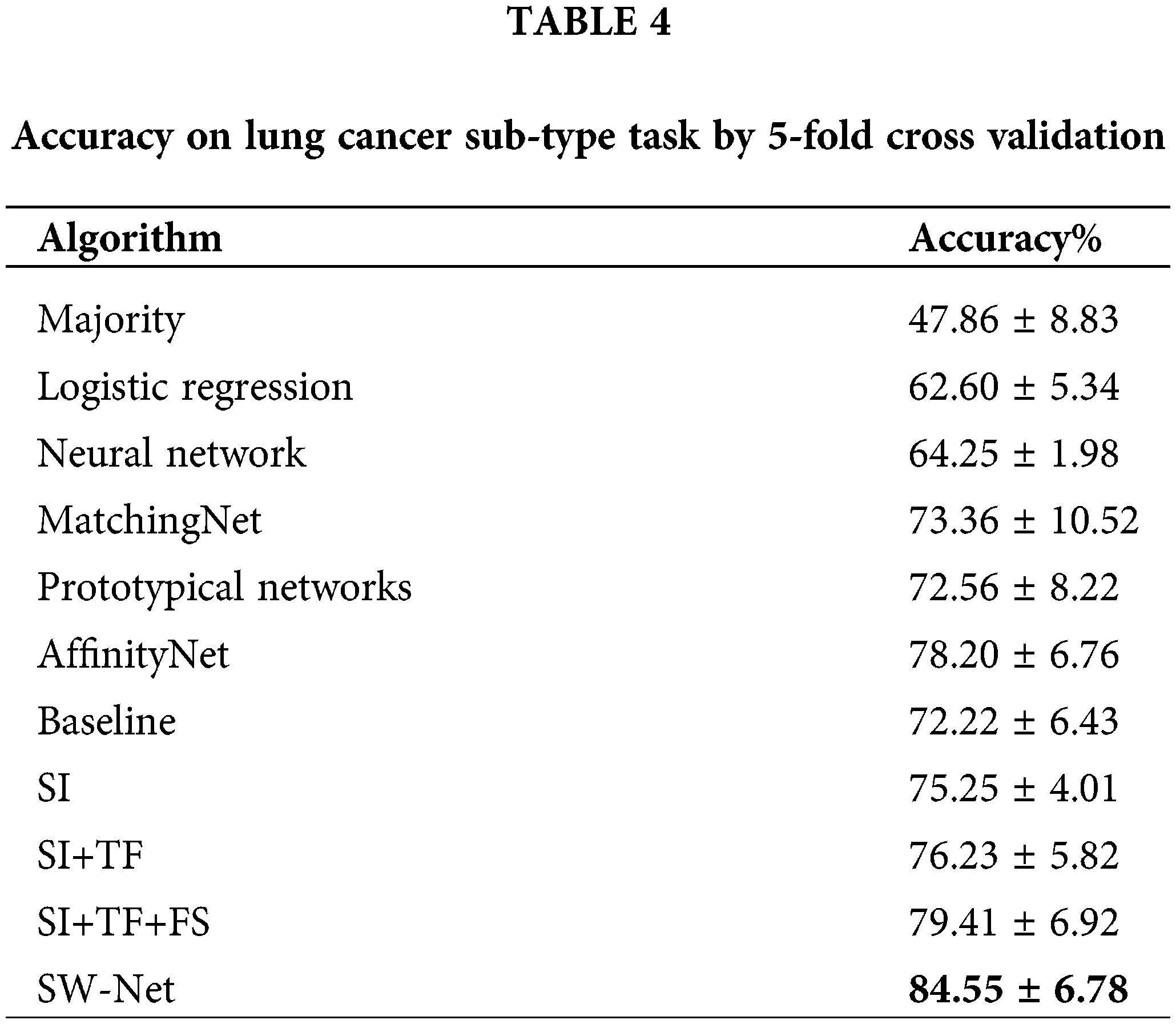
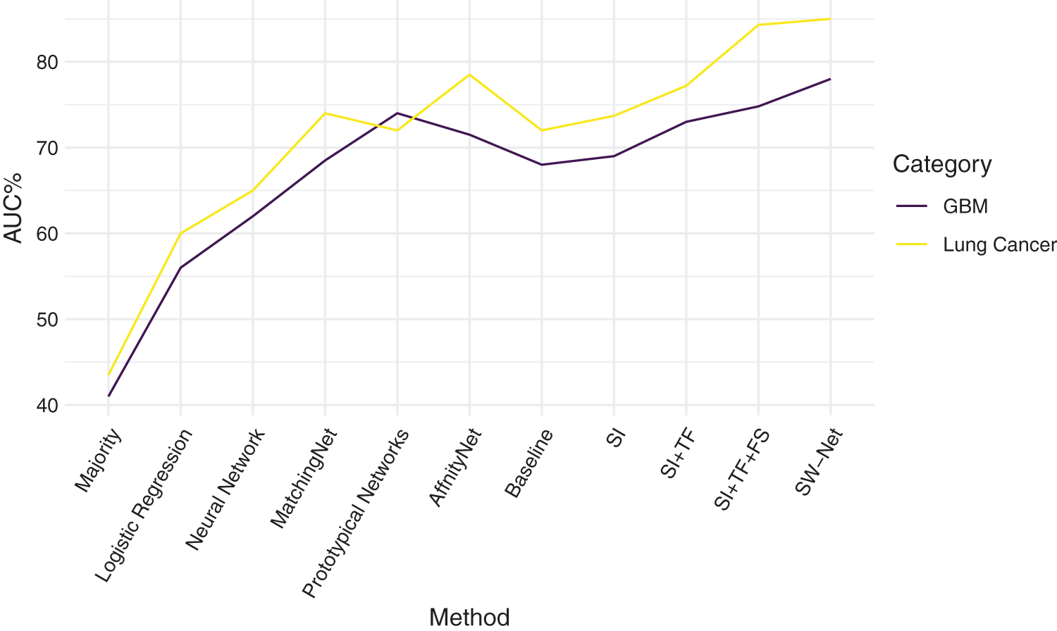
Figure 5: Comparison of Area Under the ROC curve on Lung Cancer task and glioblastoma multiforme (GBM) task.

Fig. 6 presents the effect of changing the query shot on the mean accuracy of the tasks for 1 support shot and 5 support shots. For the 1 support shot experiment, the Shannon entropy penalty term in SW-Net resulted in an increase in prediction accuracy as the query shot increased. This effect was not obvious in the 5-support shot setting because more labeled data in the support set is available. One interesting point we observed is that 1 query shot gets a higher result because our transductive fine-tuning method can adapt to the few query samples. The 1 query shot is enough to benefit from this method.

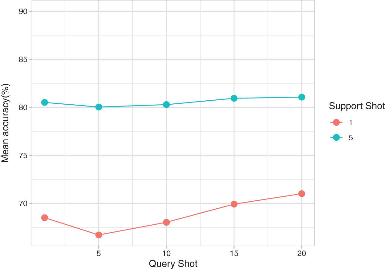
Figure 6: Mean accuracy of SW-Net for different query shots and support shots.

To further test the feature selection capability of the SW-Net, we selected 20 top-ranked significant genes of the lung cancer sub-type task with SW-Net and draw the Kaplan-Meier (KM) curve (Cerami et al., 2012) with cBioPortal https://www.cbioportal.org as shown in Fig. 7. Survival analysis of the selected important genes is performed based on the Pan-Cancer Atlas dataset (Hoadley et al., 2018). The two curves do not intersect. The Log-rank test p-value was 4.387e-4. The blue line, which represents the unaltered group of patients in the selected genes, has a longer survival time.

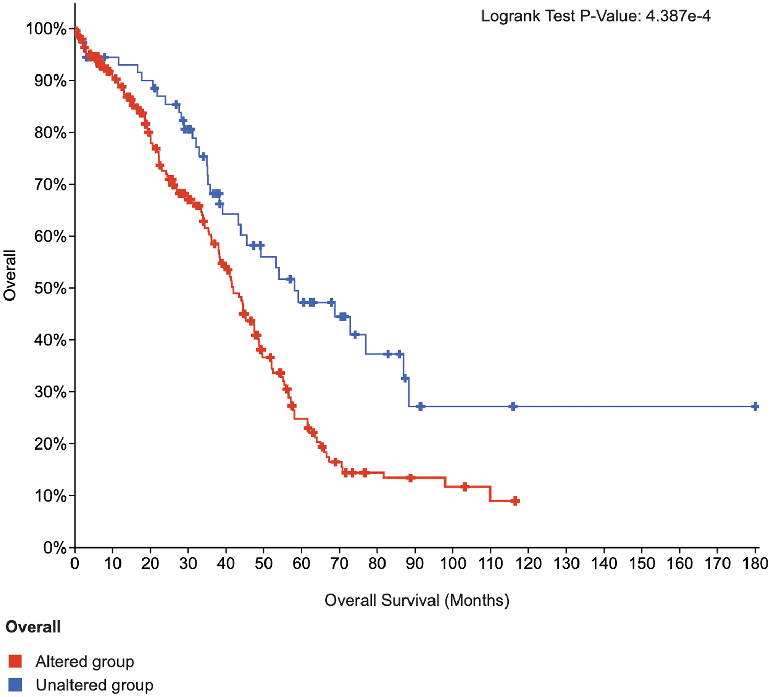
Figure 7: K-M curves of 20 top-ranked genes of lung cancer selected by SW-Net.

Moreover, we experimented on the lung cancer dataset to investigate the significance of the important genes selected by our model. We selected the 50 top-ranked genes and performed enrichment analysis with Metascape (Zhou et al., 2019). The database we use includes WikiPathway (Slenter et al., 2018) and Rectome Pathway (Fabregat et al., 2018).

Fig. 8 shows that they are enriched in the “non-small cell lung cancer” pathway. Signaling by epidermal growth factor receptor (EGFR) and cytokine signaling in the immune system are also related to lung cancer. Tuberculosis, which has been proven to be associated with lung cancer (Wu et al., 2011; Yu et al., 2011), is enriched in the enrichment analysis in our experiment. Other enriched pathways include fms-like tyrosine kinase 3 (FLT3) signaling, S phase, and so on, which are associated with the cell cycle (Sage et al., 2003). EGF and EGFR play a vital role in the development of cancer proliferation (Huang et al., 2014).

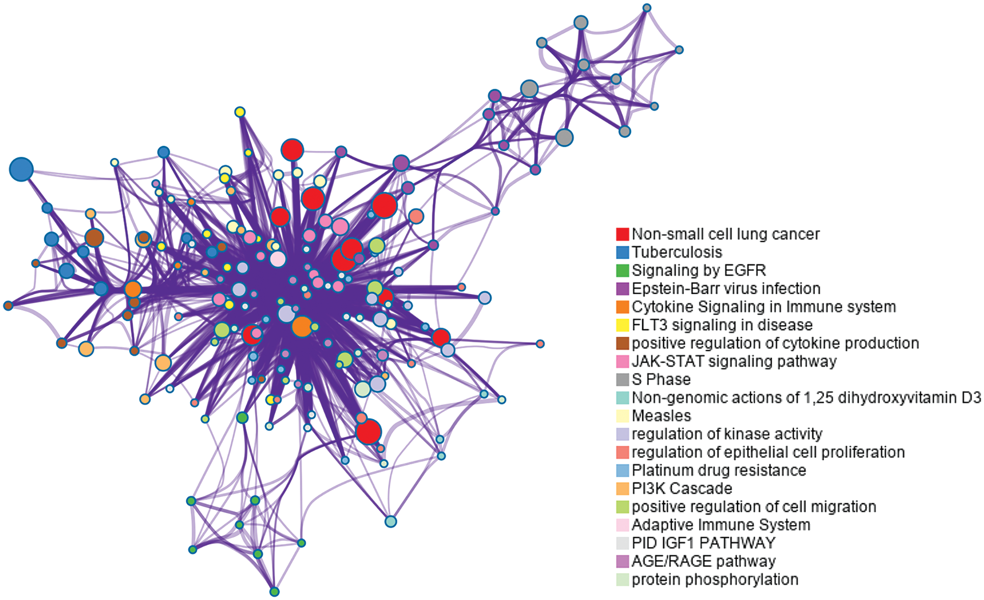
Figure 8: Enrichment analysis for the 50 top ranked genes by meta-learning with the reweighting method in the lung cancer dataset.

Discussion and Conclusion

Most computational methods are developed for one particular clinical task in isolation. For example, (van Wieringen et al., 2009) worked on survival prediction. Lyu and Haque (2018) researched on tumor cell type classification. This is quite different from the real clinical process. Clinicians and doctors need to take several clinical variables into account simultaneously. In other words, these tasks are interrelated with each other. We can get a more reliable result if we have comprehensive knowledge about the patient. It is practical to take relative tasks into account to get more precise prediction accuracy. We utilized a collection of interrelated tasks and build some prior knowledge for the general prediction. Our new SW-Net can achieve competitive disease sub-type prediction accuracy compared to other traditional methods because we considered the correlated tasks.

What’s more, the ability of our model to prioritize the genes for survival analysis was validated by experiments. We performed gene set enrichment analysis. The top-ranked genes were enriched in crucial cancer pathways, such as cell cycle, cell death, interleukin, cytokine signaling in the immune system, and so on. Besides the well-known cancer pathways, our experiment reveals that viruses can be a potential factor affecting cancer development, which is not well-studied yet. For lung cancer, the Epstein-Barr virus infection pathway is enriched, which also reveals that hepatotropic viruses may be associated with lung cancer. In recent research, it has been found that hepatotropic viruses are related to advanced non-small cell lung cancer (Zapatka et al., 2020).

In conclusion, the small data and high noise are crucial problems researchers encounter when analyzing genomic data. To address this issue, we utilized a modified approach with a reweighting strategy, which can learn from a small number of samples, and the reweighting module suppressed the samples with high noise. We demonstrate that the proposed framework can achieve competitive performance with traditional methods and other complex models. Last, experiments show that the proposed method is interpretable. The top-ranked genes of lung cancer are enriched in biological pathways associated with cancers.

The small data issue is a factor that limits many biomedical analyses. Our work further demonstrates the prospect of meta-learning for solving biomedical problems with small data. In the future, we want to explore the applications of meta-learning for other biomedical problems, including cancer subtype prediction, drug discovery, and medical image analysis.

Availability of Data and Materials: The datasets generated during and/or analysed during the current study are available from the corresponding author on reasonable request.

Author Contribution: Study conception and design: Yuhan Ji and Yong Liang; data collection: Yuhan Ji and Ziyi Yang; analysis and interpretation of results: Yuhan Ji and Ning Ai; draft manuscript preparation: Yuhan Ji, Yong Liang, Ziyi Yang, and Ning Ai. All authors reviewed the results and approved the final version of the manuscript.

Ethics Approval: Not applicable.

Funding Statement: This work is supported by the Macau Science and Technology Development Funds Grands No. 0158/2019/A3 from the Macau Special Administrative Region of the People’s Republic of China.

Conflicts of Interest: The authors declare that they have no conflicts of interest to report regarding the present study.

References

Bertinetto L, Henriques JF, Torr PH, Vedaldi A (2018). Meta-learning with differentiable closed-form solvers. arXiv preprint arXiv:1805.08136. [Google Scholar]

Cerami E, Gao J, Dogrusoz U, Gross B, SumS O, Aksoy B, Schultz N. (2012). The cBio cancer genomics portal: an open platform for exploring multidimensional cancer genomics data. Cancer Discovery 2: 401–404. [Google Scholar]

Chen WY, Liu YC, Kira Z, Wang YCF, Huang JB (2019). A closer look at few-shot classification. arXiv preprint arXiv:1904.04232. [Google Scholar]

Dai Z, Yang Z, Yang F, Cohen WW, Salakhutdinov RR (2017). Good semi-supervised learning that requires a bad gan. Proceedings of the 31st International Conference on Neural Information Processing Systems, pp. 6513–6523. Long Beach. [Google Scholar]

de la Torre F, Black MJ (2003). A framework for robust subspace learning. International Journal of Computer Vision 54: 117–142. DOI 10.1023/A:1023709501986. [Google Scholar] [CrossRef]

Fabregat A, Jupe S, Matthews L, Sidiropoulos K, Gillespie M, Garapati P, Haw R, Jassal B, Korninger F, May B (2018). The reactome pathway knowledgebase. Nucleic Acids Research 46: D649–D655. DOI 10.1093/nar/gkx1132. [Google Scholar] [CrossRef]

Li FF, Fergus R, Perona P (2006). One-shot learning of object categories. IEEE Transactions on Pattern Analysis and Machine Intelligence 28: 594–611. DOI 10.1109/TPAMI.2006.79. [Google Scholar] [CrossRef]

Finn C, Abbeel P, Levine S (2017). Model-agnostic meta-learning for fast adaptation of deep networks. International Conference on Machine Learning, pp. 1126–1135. Sydney. [Google Scholar]

Freund Y, Schapire RE (1997). A decision-theoretic generalization of on-line learning and an application to boosting. Journal of Computer and System Sciences 55: 119–139. DOI 10.1006/jcss.1997.1504. [Google Scholar] [CrossRef]

Garcia V, Bruna J (2017). Few-shot learning with graph neural networks. arXiv preprint arXiv:1711.04043. [Google Scholar]

Grandvalet Y, Bengio Y (2004). Semi-supervised learning by entropy minimization. Proceedings of the 17th International Conference on Neural Information Processing Systems, pp. 529–536. Cambridge. [Google Scholar]

Hoadley KA, Yau C, Hinoue T, Wolf DM, Lazar AJ et al. (2018). Cell-of-origin patterns dominate the molecular classification of 10,000 tumors from 33 types of cancer. Cell 173: 291–304. DOI 10.1016/j.cell.2018.03.022. [Google Scholar] [CrossRef]

Huang P, Xu X, Wang L, Zhu B, Wang X, Xia J (2014). The role of EGF-EGFR signalling pathway in hepatocellular carcinoma inflammatory microenvironment. Journal of Cellular and Molecular Medicine 18: 218–230. DOI 10.1111/jcmm.12153. [Google Scholar] [CrossRef]

Jiang L, Meng D, Mitamura T, Hauptmann AG (2014). Easy samples first: Self-paced reranking for zero-example multimedia search. Proceedings of the 22nd ACM International Conference on Multimedia, pp. 547–556. Orlando. [Google Scholar]

Kipf TN, Welling M (2016). Semi-supervised classification with graph convolutional networks. arXiv preprint arXiv:1609.02907. [Google Scholar]

Kumar M, Packer B, Koller D (2010). Self-paced learning for latent variable models. Proceedings of the 23rd International Conference on Neural Information Processing Systems, vol. 1, pp. 1189–1197. Vancouver. [Google Scholar]

Lee K, Maji S, Ravichandran A, Soatto S (2019). Meta-learning with differentiable convex optimization. Proceedings of the IEEE/CVF Conference on Computer Vision and Pattern Recognition, pp. 10657–10665. Long Beach. [Google Scholar]

Liang Y, Liu C, Luan XZ, Leung KS, Chan TM, Xu ZB, Zhang H (2013). Sparse logistic regression with a L 1/2 penalty for gene selection in cancer classification. BMC Bioinformatics 14: 1–12. DOI 10.1186/1471-2105-14-198. [Google Scholar] [CrossRef]

Lin TY, Goyal P, Girshick R, He K, Dollár P (2020). Focal loss for dense object detection. IEEE Transactions on Pattern Analysis and Machine Intelligence 42: 318–327. DOI 10.1109/TPAMI.2018.2858826. [Google Scholar] [CrossRef]

Liu J, Lichtenberg T, Hoadley KA, Poisson LM, Lazar AJ et al. (2018). An integrated TCGA pan-cancer clinical data resource to drive high-quality survival outcome analytics. Cell 173: 400–416. DOI 10.1016/j.cell.2018.02.052. [Google Scholar] [CrossRef]

Lyu B, Haque A (2018). Deep learning based tumor type classification using gene expression data. Proceedings of the 2018 ACM International Conference on Bioinformatics, Computational Biology, and Health Informatics. Association for Computing Machinery, pp. 89–96. New York. [Google Scholar]

Ma T, Zhang A (2019). AffinityNet: Semi-supervised few-shot learning for disease type prediction. Proceedings of the AAAI Conference on Artificial Intelligence, vol. 33, pp. 1069–1076. Honolulu. [Google Scholar]

Mishra N, Rohaninejad M, Chen X, Abbeel P (2018). A simple neural attentive meta-learner. arXiv preprints, arXiv:1707.03141. [Google Scholar]

Munkhdalai T, Yu H (2017). Meta networks. Proceedings of the 34th International Conference on Machine Learning, pp. 2554–2563. Sydney. [Google Scholar]

Nair V, Hinton GE (2010). Rectified linear units improve restricted boltzmann machines. Proceedings of the 27th International Conference on International Conference on Machine Learning, pp. 807–814. Haifa. [Google Scholar]

Nichol A, Achiam J, Schulman J (2018). On first-order meta- learning algorithms. arXiv preprint arXiv:1803.02999. [Google Scholar]

Qiu YL, Zheng H, Devos A, Selby H, Gevaert O (2018). Low-shot learning with imprinted weights. Proceedings of the IEEE Conference on Computer Vision and Pattern Recognition, pp. 5822–5830. Salt Lake City. [Google Scholar]

Qiu YL, Zheng H, Devos A, Selby H, Gevaert O (2020). A meta-learning approach for genomic survival analysis. Nature Communications 11: 6350. DOI 10.1038/s41467-020-20167-3. [Google Scholar] [CrossRef]

Rukhsar L, Bangyal WH, Ali Khan MS, Ag Ibrahim AA, Nisar K, Rawat DB (2022). Analyzing RNA-seq gene expression data using deep learning approaches for cancer classification. Applied Sciences 12: 1850. DOI 10.3390/app12041850. [Google Scholar] [CrossRef]

Rusu AA, Rao D, Sygnowski J, Vinyals O, Pascanu R, Osindero S, Hadsell R (2018). Meta-learning with latent embedding optimization. arXiv preprint arXiv:1807.05960. [Google Scholar]

Sage J, Miller AL, Pérez-Mancera PA, Wysocki JM, Jacks T (2003). Acute mutation of retinoblastoma gene function is sufficient for cell cycle re-entry. Nature 424: 223–228. DOI 10.1038/nature01764. [Google Scholar] [CrossRef]

Samiei M, Würfl T, Deleu T, Weiss M, Dutil F, Fevens T, Boucher G, Lemieux S, Cohen JP (2019). The tcga meta-dataset clinical benchmark. arXiv preprint arXiv:1910.08636. [Google Scholar]

Saria S, Goldenberg A (2015). Subtyping: What it is and its role in precision medicine. IEEE Intelligent Systems 30: 70–75. DOI 10.1109/MIS.2015.60. [Google Scholar] [CrossRef]

Shu J, Xie Q, Yi L, Zhao Q, Zhou S, Xu Z, Meng D (2019). Meta-weight-net: Learning an explicit mapping for sample weighting. Proceedings of the 33rd International Conference on Neural Information Processing Systems, pp. 1919–1930. Vancouver. [Google Scholar]

Slenter DN, Kutmon M, Hanspers K, Riutta A, Windsor J, Nunes N, Mélius J, Cirillo E, Coort SL, Digles D (2018). WikiPathways: A multifaceted pathway database bridging metabolomics to other omics research. Nucleic Acids Research 46: D661–D667. DOI 10.1093/nar/gkx1064. [Google Scholar] [CrossRef]

Snell J, Swersky K, Zemel R (2017). Prototypical networks for few-shot learning. Proceedings of the 31st International Conference on Neural Information Processing Systems, pp. 4080–4090. Long Beach. [Google Scholar]

Sohn BH, Hwang JE, Jang HJ, Lee HS, Oh SC et al. (2017). Clinical significance of four molecular subtypes of gastric cancer identified by the cancer genome atlas project. Clinical Cancer Research 23: 4441–4449. DOI 10.1158/1078-0432.CCR-16-2211. [Google Scholar] [CrossRef]

Sung F, Yang Y, Zhang L, Xiang T, Torr PH, Hospedales TM (2018). Learning to compare: Relation network for few-shot learning. Proceedings of the IEEE Conference on Computer Vision and Pattern Recognition, pp. 1199–1208. Salt Lake City. [Google Scholar]

van Wieringen WN, Kun D, Hampel R, Boulesteix AL (2009). Survival prediction using gene expression data: A review and comparison. Computational Statistics & Data Analysis 53: 1590–1603. DOI 10.1016/j.csda.2008.05.021. [Google Scholar] [CrossRef]

Vinyals O, Blundell C, Lillicrap T, Wierstra D (2016). Matching networks for one shot learning. Proceedings of the 30th International Conference on Neural Information Processing Systems, pp. 3637–3645. Red Hook. [Google Scholar]

Wang Y, Kucukelbir A, Blei DM (2017). Robust probabilistic modeling with bayesian data reweighting. Proceedings of the 34th International Conference on Machine Learning, pp. 3646–3655. Sydney. [Google Scholar]

Weiss K, Khoshgoftaar TM, Wang D (2016). A survey of transfer learning. Journal of Big Data 3: 1–40. DOI 10.1186/s40537-016-0043-6. [Google Scholar] [CrossRef]

Wu CY, Hu HY, Pu CY, Huang N, Shen HC, Li CP, Chou YJ (2011). Pulmonary tuberculosis increases the risk of lung cancer: A population­based cohort study. Cancer 117: 618–624. DOI 10.1002/cncr.25616. [Google Scholar] [CrossRef]

Yang Z, Shu J, Liang Y, Meng D, Xu Z (2020). Select-ProtoNet: Learning to select for few-shot disease subtype prediction. arXiv preprint arXiv:2009.00792. [Google Scholar]

Yoo TK, Choi JY, Kim HK (2021). Feasibility study to improve deep learning in OCT diagnosis of rare retinal diseases with few-shot classification. Medical & Biological Engineering & Computing 59: 401–415. DOI 10.1007/s11517-021-02321-1. [Google Scholar] [CrossRef]

Yu YH, Liao CC, Hsu WH, Chen HJ, Liao WC, Muo CH, Sung FC, Chen CY (2011). Increased lung cancer risk among patients with pulmonary tuberculosis: A population cohort study. Journal of Thoracic Oncology 6: 32–37. DOI 10.1097/JTO.0b013e3181fb4fcc. [Google Scholar] [CrossRef]

Zapatka M, Borozan I, Brewer DS, Iskar M, Grundhoff A, Alawi M, Desai N, Sültmann H, Moch H, Cooper CS (2020). The landscape of viral associations in human cancers. Nature Genetics 52: 320–330. DOI 10.1038/s41588-019-0558-9. [Google Scholar] [CrossRef]

Zhou Y, Zhou B, Pache L, Chang M, Khodabakhshi AH, Tanaseichuk O, Benner C, Chanda SK (2019). Metascape provides a biologist-oriented resource for the analysis of systems-level datasets. Nature Communications 10: 1–10. DOI 10.1038/s41467-019-09234-6. [Google Scholar] [CrossRef]