PSTCNN: Explainable COVID-19 diagnosis using PSO-guided self-tuning CNN

Introduction

COVID-19 is a new global epidemic characterised by high infectivity and variability, posing a significant threat to human life and the global economy (Chakraborty and Maity, 2020). The pathogen of COVID-19 is severe acute respiratory syndrome coronavirus 2 (SARS-CoV-2) (Hasöksüz et al., 2020), a single-stranded RNA virus of the genus Beta coronavirus and shares 79% nucleotide sequence identity with SARS-CoV, the causative agent of the 2002 SARS epidemic. Other viruses in the same genus include human coronavirus HCoV-HKu1, HCoV-OC43, and Middle East respiratory syndrome coronavirus (MERS-CoV). These coronavirus particles are composed of four structural proteins, including nucleocapsid (N), membrane (M), envelope (E), and spike (S) proteins. The S protein mediates the attachment and fusion of the coronavirus to the host cell membrane. The S protein consists of two non-covalently related subunits: (1) the S2 subunit anchors the S protein to the host cell membrane, and (2) the S1 subunit binds to its specific angiotensin-converting enzyme 2 (ACE2) receptor to enter the cell and infect patients (Jackson et al., 2022). The new coronavirus is highly infectious. The number of confirmed COVID-19 diagnoses has been growing since first identified in 2019. As of April 2022, the cumulative number of confirmed COVID-19 diagnoses is close to five billion, with over six million deaths (Organization, 2022). At the same time, the novel coronavirus continues to mutate at a much faster rate than the vaccine development. In addition, it has undergone significant changes in its characteristics, making it challenging to sustain efforts to combat the disease.

Symptoms of COVID-19 vary significantly among individuals with a continuous cough, fever, taste loss, and, in severe cases, death, thus making COVID-19 even more dangerous. In general, the spread of infectious diseases can be stopped by isolating the source of infection and blocking the transmission route. However, because of (1) the mutation of the new coronavirus, (2) the increase in the number of asymptomatic patients, and (3) the difficulties of diagnosis, isolating the source of COVID-19 infection becomes a challenge (Kronbichler et al., 2020).

The most widely used test for COVID-19 is the reverse transcription polymerase chain reaction (RT-PCR) (van Kasteren et al., 2020), which has improved considerably in recent years, allowing results to be obtained within tens of minutes. However, these tests are often associated with high false negatives and a high potential for underdiagnosis (Arevalo-Rodriguez et al., 2020). Moreover, the availability of RT-PCR reagents is highly challenging due to the high number of infections and the population's fears of a global disease. Therefore, exploring more effective ways of diagnosing COVID-19 for outbreak control is essential.

COVID-19 is an infectious emergency respiratory disease, and the disease state is usually reflected in the lungs. X-ray and CT, the most common medical imaging techniques in modern medicine, can play a vital role in diagnosing COVID-19 by reflecting changes in the lung tissue through their chest impact. As a relatively new technology, computed tomography (CT) imaging allows multi-layered photography of the target area to form a three-dimensional image, providing multi-angle image data with a higher resolution than X-ray images (Berrimi et al., 2021). Therefore, the diagnosis of COVID-19 by CT imaging of the chest has significant research and practical value. However, the diagnosis of chest CT is often dependent on medical specialists, making it difficult to be helpful in the face of the shortage of medical resources associated with a COVID-19-like global epidemic.

As one of the most influential frontier technologies of the 20th century, artificial intelligence (AI) significantly impacts human work and life (Liang et al., 2021), especially in the medical field (Han et al., 2022; Miller et al., 2022; Ning et al., 2020). Artificial intelligence-based computer-aided diagnosis (CAD) is one of the research areas receiving the most attention (Chen et al., 2022; Guan et al., 2022; Yu et al., 2022a; Yu et al., 2022b). In the face of the global pandemic of COVID-19, many researchers have risen to fight against it, hoping to contribute to its eradication. As a result, many studies on COVID-19 are rapidly emerging (Bobermin et al., 2022; Carretta et al., 2022; Ozturk and Kara, 2022), especially on COVID-19 CAD systems.

Chen (2021) used the effectiveness of the greyscale co-occurrence matrix (GLCM) for texture feature extraction to extract features from chest CT images and a support vector machine (SVM) to perform binary classification on these features to achieve the diagnosis of COVID-19. Pi and Lima (2021) and Pi (2021) also used GLCM as a feature extraction method. Among them, Pi and Lima (2021) used the extreme learning machine (ELM) as a classifier to classify the features extracted from chest CT by GLCM, and Pi (2021) used the Schmitt Neural Network as the classifier of the model. These methods achieved promising performance, which demonstrates the effectiveness of GLCM for feature extraction from chest CT images. Some methods extract features using wavelet entropy. The study by Wang (2021) used Jaya algorithm-based training algorithm to train the model and achieved an encouraging performance. A further attempt by Wang et al. (2022) to use the Self-Adaptive Jaya (SAJ) algorithm to train their model. Their model (WE-SAJ) has achieved further performance improvements. On the other hand, Field Wu (Wu, 2020) used a particular wavelet entropy, Wavelet Renyi Entropy, as the feature extraction method and a three-stage biogeographic optimisation algorithm as the training algorithm, achieving excellent performance. Khan (2021) proposed a novel deep-learning approach to construct a diagnostic tool for COVID-19. They used Pseudo-Zernike moment derived from Zernike moment as feature values and deep sparse autoencoder as the classifier for chest CT image classification. Their model obtained an accuracy higher than 90% and achieved similarly excellent performance in other performance metrics. Some studies have also used models based on classical deep-learning methods to diagnose COVID-19. Hou and Han (2022) used a six-layer convolutional neural network (CNN) for chest CT images based COVID-19 diagnosis task. Their model has achieved about 90% accuracy. Yu et al. (2020) improved one of the most classical CNNs, GoogleNet, for the COVID-19 chest CT image-based diagnosis task. They replaced the last two layers of GoogleNet with a dropout layer, two fully connected layers, and an output layer. Their model also achieved close to 90% accuracy. Zhang et al. (2021) proposed a multi-input deep convolutional attention network constructed using a convolutional block attention module. Their model has achieved more than 90% accuracy. These models are well-designed but require hyperparameter tuning to achieve fast convergence and high performance, often requiring expert intervention. At the same time, manual tuning of hyperparameters often relies on empirical knowledge, which is subjective and requires a high level of expertise. These factors have primarily hindered the cross-domain generalisation of CAD methods. We believe an optimisation algorithm could be a solution to make the hyperparameter tuning process automatic.

This paper uses the particle swarm optimisation algorithm (PSO) to optimise the three hyperparameters and gradient-based localisation of CNN to generate visual explanations. The proposed approach uses particle swarm optimisation algorithms to perform auto hyperparameters tuning, reducing the dependence of model construction on machine learning experts. In addition, PSO purposefully finds the hyperparameters closest to the optimal solution more consistently. Our method has achieved a promising performance in COVID-19 diagnosis.

Our contributions to this study are as follows: (i) we experimentally demonstrated the possibility of using optimisation algorithms for hyperparameter tuning, (ii) we proposed a high-performance COVID-19 diagnostic method with a visual explanation based on CT chest images, and (iii) we further explored the potential of AI-based techniques in medical image processing. In the rest of the paper, Section 2 introduces the data set used, Section 3 introduces the background of the methods involved in the experiment, Section 4 describes the experimental workflow of PSO-guided self-tuning CNN (PSTCNN), and Section 5 presents the experiment results and discusses it in detail.

Dataset

The experiment used a publicly available chest CT image slice dataset proposed by Zhang et al. (2022). The dataset was a binary classification dataset with the categories positive (COVID-19) and negative (Health Control). The dataset contains a total of 296 slice images. The positive category contains 148 slice images taken from chest CT images of 66 COVID-19-infected subjects, assessed as positive by nucleic acid test. The negative category contains 148 slice images taken from chest CT images of 66 uninfected subjects from COVID-19. These subjects included 77 males and 55 females. The detailed statistic of the dataset is shown in Table 1, and two sample images are illustrated in Fig. 1.

Figure 1: COVID-19 infected Chest-computed tomography (CT) slice image sample (a) and uninfected Chest-CT slice image sample (b).

Methodology

10-Fold cross validation

The dataset used for the study was small, so we introduced the 10-Fold Cross Validation to train and evaluate the model. Specifically, we divided the dataset into ten groups and performed ten runs, with different groups selected as the test set and all other groups as the training set for each run. The model was thoroughly trained and evaluated for each run to obtain performance metric values. The final performance of the model was obtained by calculating the sum, the mean and standard deviation (MSD) of all ten sets of performance metric values. This approach allowed for efficient use of the samples in the dataset and effectively avoided overfitting.

Feature learning through convolutional neural network

CNN is one of the trendiest research directions in computer-aided diagnosis tasks. It comprises different network layers, e.g., the input layer, convolutional layer, activation layer, pooling layer, and output layer. By combining these network layers, CNNs can effectively solve the problems of spatial information loss when expanding images into vectors, inefficiency training and network overfitting caused by high parameter volume when processing large images with fully connected neural networks (Gu et al., 2018).

Many existing deep learning-based CAD methods are based on CNNs. Polsinelli et al. (2020) have made a simple modification to SqueezeNet by adding a batch normalisation layer between the squeeze convolution layer and the activation layer and replacing the original rectifier linear unit (ReLU) function with an exponential linear unit (ELU) function to build a lightweight CNN model. They tested the unmodified SqueezeNet and their proposed modified model separately using a COVID-19 chest CT dataset. Their proposed modification effectively improved the performance of the model. Horry et al. (2020) used pre-trained VGG-19 based on transfer learning techniques to classify each of the three COVID-19 datasets, x-ray, CT, and ultrasound, and achieved promising results (precision up to 86% on x-ray, 100% on ultrasound and 84% on CT scans). Ismael and Şengür (2021) tested a variety of CNN models based on the COVID-19 x-ray dataset, including ResNet18 (accuracy of 88.42%), ResNet50 (accuracy of 92.63%), ResNet101 (accuracy of 87.37%), VGG16 (accuracy of 85.26%), and VGG19 (accuracy of 89.47%). Their validation of multiple pre-trained CNN models with the excellent performance of their custom CNNs further demonstrated the effectiveness of deep learning techniques for the COVID-19 diagnostic task.

Our method uses a five-layer neural network, including three convolution layers and two fully connected layers.

Convolutional layers are based on the concept of convolution. It is the core component of CNNs and generates most of the computation in the network. A convolutional layer contains a number of learnable filters (kernels), where the kernels are usually squares with smaller widths and lengths but the same depth as the input image. The convolution is the process by which the kernel slides over the image. The sliding direction is from left to right for the width direction and then repeats sliding following the width direction from the top rows to the bottom rows of the image until reaching the bottom edge of the image. For each step of the sliding process of the convolution, each pixel of the region mapped by the kernel in the input image is multiplied by the information at the location corresponding to the flipped kernel. All the results generated are summed to aggregate the information. The region mapped by the kernel in the input image is called the sliding window. The step size of the sliding, S=(Sl,Sw) , is a customisable hyperparameter, in which Sl represents the step size of the sliding across the length direction and Sw represents the step size of the sliding across the width direction.

In this process, the filters scan across the input image, so every neighbourhood of the image is processed by the same filter. This sharing weight feature reduces the number of parameters, thus reducing computational costs and preventing overfitting due to too many parameters. Assume the size of kernel K is F×F , and the size of a two-dimension single-channel image I is Nl×Nw , where Nl represents the length of I , and Nw represents the width of I .

The output o(m,n) of the sliding process of the convolution when the sliding window centred at (m,n) can be defined as presented in Eq. (1). Let O be the output of the convolution, o∈O . Repeating the calculation to slide throughout the entire image will generate the output O of the convolution. If there are residuals (the sliding window cannot reach the edge of the image), the residual image pixels are abandoned. The output shape, Z=(Zl,Zw,Zc), of a convolutional layer can be calculated by Eq. (2).

o(m,n)=∑a=0F−1∑b=0F−1K[a,b]⋅I[n+⌊F2⌋−a,m+⌊F2⌋−b], (1)

where (n,m) is the coordinate of the pixel point corresponding to the position of the centre of the sliding window in the input image. The range of n∈N is (F2,Nw−F2−1) , and the range of m∈N is (F2,Nl−F2−1) .

Z=(Zl,Zw,Zc)=(⌊Nl−FSl⌋+1,⌊Nw−FSw⌋+1,Zc), (2)

where Zl , Zw , and Zc represent the length, width, and number of channels of the output O , respectively. Nl and Nw represent the length and width of the input image, respectively. F×F is the size of the kernel.

Activation functions play an essential role in CNNs, bringing a non-linear factor to the neural network, enhancing its expressive power, and thus improving the final classification performance. Working with high-dimensional input data such as images would be computationally prohibitive for each neuron in a network layer to fully connect to all the neurons in the previous layer (Najafabadi et al., 2015). Therefore, neurons in a CNN are usually related to only one local region of the input data. The spatial size of this connected region is called the neuron’s receptive field, which depends on the kernel’s size and is a hyperparameter. Also, to give the network the ability to handle non-linear tasks, the convolutional layer often includes an activation function as a non-linear factor. The most common activation function is the ReLU function. In addition, the ReLU activation function can be used to construct sparse matrices to remove redundancy from the data and retain the maximum possible features of the data. The formula for the ReLU function is shown in Eq. (3).

f(x)={x,         x>0,0,    otherwise. (3)

Applying Eq. (3) to every pixel of O generates O′ , the output of the ReLU activation layer, as shown in Eq. (4).

O′(a,b)=f(O(a,b)), (4)

where (a,b) is the coordinate of pixels in O , in which 0≤a<Ow , a∈N , 0≤b<Ol , b∈N . Each pixel in O′ corresponds to a pixel in O but with a new value generated by the ReLU function with an input of the pixel’s value in O . O′ has the same size and shape as O .

Padding can regulate the size of the output of the network layer. In the convolution process, pixels at the edges of input images are never located in the centre of the kernel. These pixels are used far less than the pixels in the centre of the image, resulting in a significant loss of information at the image boundaries. In addition, the output image from the convolution process often does not maintain the same size as the input image, and different kernel sizes result in various degrees of image shrinkage. Padding is designed to address this issue, which has two modes, VALID mode and SAME mode.

In the VALID mode, padding does not perform any operations, and convolution performs a basic convolution operation, where the output image size is smaller than the input image. In the SAME mode, additional pixels are padded around the input image according to the kernel size (the padding value is usually 0). It allows the kernel to extend beyond the original image boundaries, thus allowing the output image to remain the same size as the original and avoiding losing information from the edges of the input image. Fig. 2 illustrates convolution samples under VALID and SAME padding, respectively. Our method uses the SAME padding to preserve the image edge information, keeping the same size as the original image.

Figure 2: In the VALID mode (a), the output size of the convolution for a 5 × 5 image is 3 × 3. In SAME mode (b), the input image is padded to size 6 × 6, and the output size remains the same as the original input, 5 × 5. The dotted blocks are the padded section.

Training algorithm

Training algorithms can determine the way how neural networks run. The essence of deep learning is to (1) take the loss function as the objective function, (2) input a large amount of data, (3) calculate the value of the objective function, and then (4) adjust and optimise the learnable parameters in the model to obtain the model that will give the closest result to the true value. In this process, the optimiser algorithm was followed. The choice of optimiser plays a vital role in deep learning training, as it affects the speed of convergence of the model and the final performance achieved.

Adam (Kingma and Ba, 2014) is one of the most popular deep learning training algorithms that control the updating of model parameters. For each parameter, Adam uses the hyperparameters β1 and β2 to calculate the exponential decay rates of the past gradient gt and the square of the past gradient gt2 , respectively, dg and dgs , using first-order moment estimates and second-order moment estimates of the gradient to dynamically adjust the learning rate of each parameter. The calculation is shown in Eq. (5). As dg and dgs are initialised to 0, their values are biased towards 0. A bias correction is introduced in Adam to bias dg and dgs to obtain dg^ and dgs^ , and further offset these initial biases. The bias correction is calculated as shown in Eq. (6). Ultimately, Adam calculates the update step through the dg and dgs angles to update the parameters, as shown in Eq. (7).

dgt=β1dgt−1+(1−β1)gt,dgst=β2dgst−1+(1−β2)(gt)2, (5)

dg^=dg1−(β1)t,dgs^=dgs1−(β2)t,(6)

θt+1=θt−αd^gs+ϵd^g. (7)

Adam can adaptively adjust the learning rate of the model parameter updates, implement the step annealing process naturally, and makes the model parameter updates independent of the gradient scaling transformation. In addition, Adam has the advantages of high computational efficiency and low memory consumption (Saad Hikmat and Adnan Mohsin, 2021). In simple words, Adam can achieve typically high levels of robustness and performance in various situations (Dogo et al., 2018). Therefore, our method uses Adam as the training algorithm.

Visual explanation via gradient-based localisation (Grad-CAM)

Grad-CAM is a method for visualising the basis of CNN decisions. It uses a heat map to mark how much attention the neural network pays to different regions when classifying data, thus highlighting the regions on which the neural network focuses its attention. In detail, Grad-CAM uses the global average of the gradients to calculate the weight akc of the feature map k corresponding to the class c (as shown in Eq. (8)). then, it calculates the weighted sum of the weight and the last layer of the feature map, combining it with the ReLU activation function to produce the heat map LGradCAMc . The procedure for calculating the heat map is shown in Eq. (9).

αkc=1z∑i∑j∂yc∂Aijk, (8)

where z is the number of pixels in the feature map, yc is the fraction corresponding to class c , and Aijk denotes the pixel values at the coordinate (i,j) of the k feature maps.

LGradCAMc=f(∑kakcAk), (9)

where f represents the ReLU function.

Hyperparameter tuning

Almost all deep learning optimisers have customisable hyperparameters that can significantly influence the performance of the optimiser, hence the speed of convergence and the ultimate performance of the model. Many studies try to optimise hyperparameter tuning for better COVID-19 diagnostics. Ezzat et al. (2021) optimised the three hyperparameters of DenseNet121, the batch size, the rate of dropout layer, and the number of neurons of the first dense layer and trained their proposed model using two sets of X-ray data from COVID-19. They could achieve 98.38% accuracy, a significant improvement over DenseNet121 (94% accuracy) and Inception-v3 (95% accuracy), which they used as controls. Monshi et al. (2021) tested the function loss, the number of epochs, and the batch size hyperparameters with different value combinations. Then, they selected the combinations of hyperparameters with the highest performance and used these combinations for the different models to test performances. In their approach, the accuracy of VGG19 improved by 11.93% and that of ResNet-50 by 4.97%. Kiziloluk and Sert (2022) used the gradient-based optimiser (GBO) and the Quasi-Newton algorithm (Q-N) to optimise the hyperparameters of several CNN models, including Alexnet, Darknet-19, Inception-v3, MobileNet, Resnet-18, and ShuffleNet. Their results show that GBO improves the classification performance of the original CNN model by 6.22%–13.29%, and the Q-N algorithm improves the performance of the original CNN model by 2.92% to 8.40%. These studies demonstrate the critical impact of hyperparameter optimisation on the performance of CNN models in COVID-19 diagnostic tasks.

However, the hyperparameters can have an infinite number of possible combinations. Therefore, hyperparameter tuning becomes a challenging, time-consuming and computationally expensive stage in training deep learning models. There is no straightforward and efficient way to accurately and quickly find the optimal hyperparameters. The most commonly used hyperparameter selection methods are Random Search and Grid Search.

Grid Search tries all the candidate hyperparameter combinations by loop traversal. Then it calculates the performance of the model under all the hyperparameter combinations and selects the parameter combination with the highest performance in the solution. However, the combination of the hyperparameters can be nearly infinite, so it is difficult to traverse all the possibilities in practical application and requires enormous time cost and calculation costs, which is inefficient.

Random Search computes a neural network with a configuration of candidate parameters by randomly sampling the parameter space and stops the search when the maximum number of iterations is completed, selecting the combination of hyperparameters with the highest performance. Although random search can be optimised to prevent repeated calculations of the same hyperparameter combinations, the search process is too random. Therefore, the large number of hyperparameter combinations makes it difficult to ensure that optimal hyperparameters are in the search range. As a result, the performance of the final model derived from random search can vary considerably for the same number of iterations.

Most hyperparameter tuning methods require many aimless attempts to find the most suitable hyperparameters, which are inefficient and ineffective, resulting in high consumption of time and computational resources. Optimisation algorithms could be a solution to this issue. This paper aims to discover the possibility of PSO in hyperparameter tuning. Table 2 discusses the advantages and disadvantages of PSO and traditional hyperparameter tuning methods from a theoretical perspective. Then, Section Table 2 introduces the experiment design of PSO-guided hyperparameter tuning.

Particle Swarm Optimisation-Guided Self-Tuning CNN

The original particle swarm optimisation

To discover more possibilities of optimisation algorithm-based hyperparameter tuning. Our experiments employed the PSO algorithm to adjust the three hyperparameters in the Adam optimiser. PSO (Kennedy and Eberhart, 1995) is an easy-to-understand and easy-to-implement optimisation algorithm with global solid search capability. Because of these advantages, it is one of the most typical optimisation algorithms. The core idea of PSO is to keep all particles moving and update their position to find the optimal solution through collaboration and information sharing among particles in the population. Hyperparameter tuning involves purposefully trying out different hyperparameter configurations and calculating the corresponding performance to find the optimal combination of hyperparameters.

Encoding scheme of particle properties

In PSO, a swarm represents the collection of all particles. Each particle pi in the swarm has two properties, a vector of velocity Vi=(vi1,vi2,⋯,vin) represents how fast a particle is moving, and a vector of position Xi=(xi1,xi2,⋯,xin) represents the direction in which a particle is moving. The algorithm finds the best position of a particle, xpbest , and the best position of the swarm, xgbest . In each iteration, the particles update their velocities in a direction for moving to new positions closer to xpbest and xgbest .

The three essential variables of the Adam training algorithm to tune to obtain the highest performance of the model (as shown in Eqs. (5)–(7)) are the learning rate α , coefficient β1 , which controls the exponential decay rates of the past gradient gt , and coefficient β2 , which controls the exponential decay rates of the square of the past gradient gt2 . The first step of our experiment is to encode these three variables into the PSO algorithm to perform tuning. Assume an n dimension search space, each particle pi has n positions (xi1,xi2,⋯,xin) and n velocities (vi1,vi2,⋯,vin) . For every position xin stores a set of hyperparameter combinations and is encoded as a vector (αin,β1in,β2in) . For every velocity, vin is encoded as a vector (v1in,v2in,v3in) , in which, v1in , v2in , and v3in are for movements of αin , β1in , and β2in , respectively. Fig. 3 illustrates the encoding scheme.

Figure 3: Illustration of Encoding Scheme. A particle swarm contains i particles, each with n positions and n velocities. Each position is a vector of α, β1, and β2, and each velocity contains three values corresponding to α, β1, and β2 of the position.

Calculations of velocities and positions

At the beginning of PSO, all particles are initialised with random positions (hyperparameter configurations) and random velocity vectors. The CNN runs iteratively in each iteration with different hyperparameter configurations. It calculates the mean squared errors (MSE) for every hyperparameter configuration as its fitness value ( F ), according to which it finds the personal best hyperparameter configuration, xpbest , for each particle, and the global best hyperparameter configuration, xgbest , of the entire particle population, which is the current best hyperparameter configuration. The formulates of finding xpbest and xgbest are shown in Eqs. (10) and (11), respectively, where xcur represents the current hyperparameter configuration.

xpbestk+1={xcur,ifF(xcur)<F(xpbestk),xpbestk,otherwise. (10)

xgbestk+1={xpbestk+1,ifF(xpbestk+1)<F(xgbestk),xgbestk,otherwise, (11)

where k represents iteration count. At the end of each iteration, the velocities of all particles are iteratively updated to directions that are closer to xpbest and xgbest , following Eq. (12). Also, the hyperparameter configurations of each particle are updated to newer values according to the new velocities, following Eq. (13).

vijk+1=vijk+cprp(xipbestk−xijk)+cgrg(xgbestk−xijk), (12)

where k represents iteration count, cp refers to the cognitive acceleration coefficient, cg refers to the social acceleration coefficient, rp and rg are random numbers.

xijk+1=xijk+vijk+1. (13)

Repeating the above steps, all particles keep moving to hyperparameter configurations that can obtain better performance until the algorithm reaches the maximum number of iterations.

Structure of particle swarm optimisation-guided self-tuning CNN

In our research, a number of experiments were performed in incremental steps to find out the neural network structure with the best performance. The final neural network is a five-layer CNN consisting of three convolution layers and two fully connected layers. A softmax function is introduced to classify the extracted features. All trainable parameters are updated following the Adam optimiser during the training process. In the tuning process, the neural networks are trained with a number of hyperparameter combinations generated or updated by PSO to obtain the performance of different combinations. Finally, the output of PSO is the hyperparameter combination of the final model with the best performance. Fig. 4 illustrates the overall structure of PSO-guided Self-Tuning CNN (PSTCNN). Theoretically, the framework can be generalised to other CNNs for image classification tasks in different domains.

Figure 4: Overall Structure of PSO-guided Self-Tuning CNN (PSTCNN). The framework can be divided into two main parts, PSO-guided Tuning (blue dashed box) and a Five-layer CNN (green dashed box). The PSO-guided Tuning part does the initialisation and updating of the parameter values. The Five-layer CNN is trained with the three hyperparameters from the PSO-guided Tuning and some pre-set constant hyperparameters (batch size is 128, kernel size is 3 × 3, and the number of epochs of 100). The MSE calculated from the output of the trained CNN is the fitness value of the PSO. The starting iteration index k = 0, and when the value of k reaches the pre-set maximum number of iterations, The training of the model is completed.

Results and Discussion

The following values were used for various performance indicators to evaluate the model’s performance comprehensively. (1) True Positive (TP) represents the number of positive samples that the model correctly predicts as the positive class, (2) True Negative (TN) represents the number of negative samples that the model correctly predicts as the negative class, (3) False Positive (FP) represents the number of negative samples that the model incorrectly predicted as the positive class, and (4) False Negative (FN) represents the number of positive samples that the model incorrectly predicts as the negative class.

The seven performance metrics used to assess the model’s performance are accuracy, precision, sensitivity, specificity, F1-score, Matthews correlation coefficient, and the Fowlkes-Mallows index, which provide a comprehensive evaluation of the model from a variety of perspectives to ensure a comprehensive performance evaluation.

Accuracy is one of the most common metrics used to evaluate the performance of a model. The core idea is to calculate the number of correct predictions as a percentage of the total number of samples, covering both positive and negative samples. The formula for accuracy is shown in Eq. (14).

Accuracy=TP+TNTP+TN+FP+FN. (14)

Although accuracy can assess the overall performance of a model with a dataset containing both positive and negative samples, it is not rigorous for an unbalanced dataset. For example, suppose there is a dataset with 90% positive samples and only 10% negative samples. A model that predicts all samples as positive can achieve 90% accuracy, but this is not an accurate representation of the model’s performance. In short, accuracy is not an effective way to evaluate the predictive performance of a model for the positive and negative samples separately, so three performance metrics, precision, sensitivity, and specificity, were introduced to provide a more comprehensive evaluation of the model.

Precision evaluates model performance primarily based on prediction results by calculating the number of samples correctly predicted as positive as a proportion of all samples predicted as positive to assess the probability that the model is correctly predicted in the samples where the model is predicted as positive. The precision of a model increases as the FP decreases, which can be a guide for finding the lowest FP. The formula of precision is shown in Eq. (15).

Precision=TPTP+FP. (15)

Specificity is another metric that can be used to measure the performance of a model for positive samples. The difference is that specificity is calculated based on the true labels of the data rather than the model predictions, and the ’performance of the model is assessed by calculating the number of samples predicted to be negative as a proportion of the total number of negative samples in the dataset. The specificity of a model also increases as the FP decreases and is calculated as shown in Eq. (16).

Specificity=TNTN+FP. (16)

Sensitivity is also calculated based on the true label of the data, except that it evaluates the model’s performance by calculating the proportion of samples predicted to be positive to the total number of positive samples in the data set. The phenomenon that sensitivity reflects is somewhat the opposite of precision. It increases as FN decreases, which can guide finding the lowest FN. Its formula is shown in Eq. (17).

Sensitivity=TPTP+FN. (17)

F1-score is the performance metric that considers both precision and sensitivity, tries to find the balance between these two metrics, and simultaneously makes them the highest possible values. The calculation of the F1-score is as shown in Eq. (18).

F1−score=2×Precision×SensitivityPrecision+Sensitivity. (18)

Matthews Correlation Coefficient (MCC) compensates that the four elements TP, TN, FP, and FN are not fully considered in the abovementioned metrics. It considers the true and predicted values as two variables and calculates the correlation coefficient. The higher the correlation between the true and predicted values, the better the model performance. An MCC value of 1 indicates a perfect positive correlation between the predicted and true results (FP=FN=0) , meaning that the model performs perfectly. An MCC value of −1 indicates a negative correlation between the predicted and true results (TP=TN=0) , meaning that the model predicts the exact opposite of the true results. An MCC of 0 means that the classifier cannot provide meaningful results. The calculation of MCC is shown in Eq. (19).

MCC=TP×TN−FP×FN(TP+FP)(TP+FN)(TN+FP)(TN+FN). (19)

The Fowlkes-Mallows Index (FMI) is a performance metric that considers both precision and sensitivity. Its calculation is as shown in Eq. (20). When FMI is 0, the value of TP is 0, which means that the model will mispredict all positive samples, and the model is not considered a valid classifier. On the other hand, if FMI is 1, the model is deemed to have perfect classification ability.

FMI=precision×sensitivity=TPTP+FP×TPTP+FN. (20)

Area Under Curve (AUC) is an important performance metric for evaluating binary classification models and is derived by calculating the area under the receiver operating characteristic (ROC) curve. The vertical and horizontal axes are true positive rate (TPR) = sensitivity and false positive rate (FPR) = specificity. The ROC curves were obtained by traversing m thresholds used to differentiate the classification results to obtain different TPR and FPR values. The more significant the decrease in FPR with increasing TPR in the curve (i.e., the steeper the ROC curve), the better the model performance. As the AUC is calculated from the area under the ROC curve, the higher the AUC, the better the model performance. As both TPR and FPR are considered, the ROC curve has the excellent quality of not changing with sample proportion, and the AUC inherits this same advantage. The AUC is calculated as shown in Eq. (21), where TPR and FPR represent a set of TPRs and a set of FPRs, respectively.

AUC=12∑i=1m−1(TPRi+TPRi−1)×(FPRi−FPRi−1). (21)

Statistical analysis

To minimise the bias in the model performance evaluation results, we used the 10-fold cross-validation to test the model’s performance under the optimal hyperparameter configuration obtained by the optimisation algorithm. As a result, we obtained a sensitivity (Sen) of 93.65% ± 1.86%, a specificity (Spc) of 94.32% ± 2.07%, a precision (Prc) of 94.30% ± 2.04%, an accuracy (Acc) of 93.99% ± 1.78%, an F1-score (F1) of 93.97% ± 1.78%, Matthews correlation coefficient (MCC) of 87.99% ± 3.56%, and Fowlkes-Mallows index (FMI) of 93.97% ± 1.78%. The 10-runs 10-fold cross-validation results are shown in Table 3.

Visual explanation

Fig. 5 illustrates three sample heatmaps generated from ten runs using Grad-CAM. The annotated parts are the basis of CNN decisions (the warmer colour and higher attention level), which correspond to COVID-19 lung infection areas. These reflect, to some extent, the soundness of the decision basis of the model.

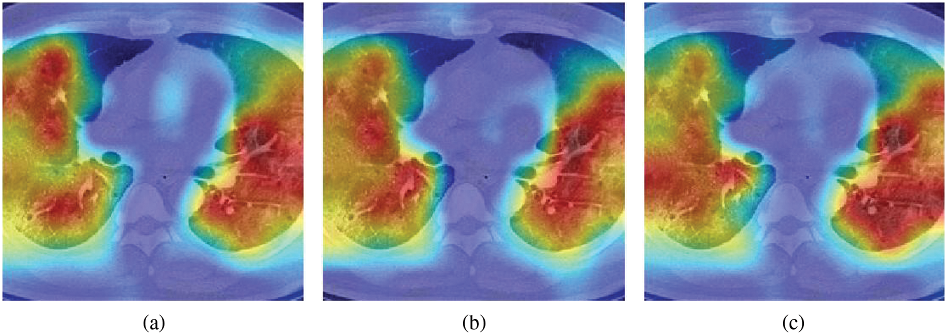
Figure 5: Heatmap examples generated by Grad-CAM.

Receiver operating characteristic curve & area under curve

Fig. 6 illustrates the ROC curve and AUC of PSTCNN. Each of the points in the figure corresponds to a threshold value. The value of the AUC can be obtained by calculating the area under the curve formed by connecting these points. The figure shows that the PSTCNN can achieve a high TPR with a low FPR and an AUC close to 0.96. These results indicate a very promising performance of the model.

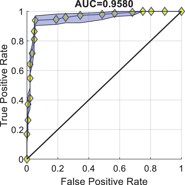
Figure 6: Receiver operating characteristic curve of particle swarm optimisation-guided self-tuning CNN.

Comparison to the state-of-the-art (SOTA)

Fig. 7 illustrates the performance comparison between our method (PSTCNN) and the deep learning-based SOTA COVID-19 diagnostic methods, where the height of the bars represents the model performance; the higher bar, the better performance. PSTCNN shows superior performance in all metrics compared to deep learning-based SOTA COVID-19 diagnostic methods. The detailed comparison is shown in Table 4. This demonstrates the feasibility of the optimisation algorithm for hyperparameter tuning. Compared to other methods, the proposed method’s comprehensive hyperparameter tuning can cover more possible combinations of hyperparameters. Furthermore, its purposeful search ensures that the global-optimal solution is approached step by step. Therefore, it can achieve better performance than manual hyperparameter tuning while automating hyperparameter tuning.

Figure 7: Comparison with state-of-the-art methods.

Conclusion

Since 2019, the global economy and human health have continuously received threats from COVID-19. In addition, the COVID-19 pandemic has highlighted the global shortage of healthcare resources. AI technologies to aid diagnosis are one of the vital viable options to alleviate this problem. This paper explores the possibility of further automation based on traditional AI techniques. It confirms this possibility by automating hyperparameter tuning using an optimisation algorithm and the excellent performance achieved by this method.

However, our method was only experimentally tested for three hyperparameters of the neural network training process, i.e., the learning rate, the coefficient that controls the exponential decay rates of the past gradient, and the coefficient that controls the exponential decay rates of the square of the past gradient. A few more hyperparameters can be tuned that we did not cover in this report, e.g., the number of network layers and the type of network layers. It means that the proposed method is insufficient as a final solution for self-tuning neural networks. In addition, the proposed method takes advantage of the purposeful movement of particles in the particle swarm optimisation algorithm for the hyperparameters to approach the optimal solution in each iteration. However, the movement of particles in each iteration is updated according to the direction of the best solution in the previous iteration, which may deviate from the global optimal solution and fall into the local optimal solution if the best solution is not in the path between the particles and the global optimal solution.

In future research, we will further explore the applicability of other optimisation algorithms to this task and attempt to avoid locally optimal solutions when obtaining combinations of hyperparameters while covering more hyperparameters in the experiment. We believe that reducing the dependence of model training on machine learning experts can effectively accelerate the generalisation of AI technologies across different domains. AI techniques will therefore become an essential tool in human life and industries in the near future.

Availability of Data and Materials: Raw data were generated at Huai’an Tongji Hospital. Derived data supporting the findings of this study are available from the corresponding author on request.

Author Contribution: Conceptualization: Wei Wang, Yanrong Pei, Shui-Hua Wang; Methodology: Wei Wang, Yu-Dong Zhang; Software: Wei Wang, Yanrong Pei, Juan Manuel Gorriz; Validation: Wei Wang, Yanrong Pei, Shui-Hua Wang, Juan Manuel Gorriz, Yu-Dong Zhang; Investigation: Wei Wan, Shui-Hua Wang, Juan Manuel Gorriz; Writing–Original Draft: Wei Wang, Yanrong Pei, Yu-Dong Zhang; Writing–Review & Editing: Wei Wang, Yanrong Pei, Yu-Dong Zhang; Visualisation: Wei Wang, Yanrong Pei, Yu-Dong Zhang; Formal analysis: Shui-Hua Wang; Resources: Shui-Hua Wang, Juan Manuel Gorriz, Yu-Dong Zhang; Supervision: Shui-Hua Wang, Juan Manuel Gorriz, Yu-Dong Zhang; Project administration: Shui-Hua Wang, Juan Manuel Gorriz, Yu-Dong Zhang; Funding acquisition: Shui-Hua Wang, Juan Manuel Gorriz, Yu-Dong Zhang.

Ethics Approval: Not applicable.

Funding Statement: This paper is partially supported by the Medical Research Council Confidence in Concept Award, UK (MC_PC_17171); Royal Society International Exchanges Cost Share Award, UK (RP202G0230); British Heart Foundation Accelerator Award, UK (AA\18\3\34220); Hope Foundation for Cancer Research, UK (RM60G0680); Global Challenges Research Fund (GCRF), UK (P202PF11); Sino-UK Industrial Fund, UK (RP202G0289); LIAS Pioneering Partnerships Award, UK (P202ED10); Data Science Enhancement Fund, UK (P202RE237); Guangxi Key Laboratory of Trusted Software, CN (kx201901).

Conflicts of Interest: The authors declare that they have no conflicts of interest to report regarding the present study.

References

Arevalo-Rodriguez I, Buitrago-Garcia D, Simancas-Racines D, Zambrano-Achig P, Campo RD et al. (2020). False-negative results of initial RT-PCR assays for COVID-19: A systematic review. PLoS One 15: 1–19. DOI 10.1371/journal.pone.0242958. [Google Scholar] [CrossRef]
Berrimi M, Hamdi S, Cherif RY, Moussaoui A, Oussalah M, Chabane M (2021). COVID-19 detection from Xray and CT scans using transfer learning. 2021 International Conference of Women in Data Science, Taif University (WiDSTaif). Taif, Saudi Arabia. [Google Scholar]
Bobermin LD, Medeiros LS, Weber F, Oliveira GTD, Santi L, Beys-da-Silva WO, GonçalveS CA, Quincozes-Santos A (2022). Impact of SARS-CoV-2 infection during pregnancy on postnatal brain development: The potential role of glial cells. BIOCELL 46: 2517–2523. DOI 10.32604/biocell.2022.021566. [Google Scholar] [CrossRef]
Carretta DM, Domenico MD, Lovero R, ArrigonI R, Wegierska AE, Boccellino M, Ballini A, Charitos IA, Santacroce L (2022). SARS-CoV-2 induced myocarditis: Current knowledge about its molecular and pathophysiological mechanisms. BIOCELL 46: 1779–1788. DOI 10.32604/biocell.2022.020009. [Google Scholar] [CrossRef]
Chakraborty I, Maity P (2020). COVID-19 outbreak: Migration, effects on society, global environment and prevention. Science of the Total Environment 728: 1–6. DOI 10.1016/j.scitotenv.2020.138882. [Google Scholar] [CrossRef]
Chen Y (2021). COVID-19 classification based on gray-level co-occurrence matrix and support vector machine. In: COVID-19: Prediction, Decision-Making, and Its Impacts, vol. 60, pp. 47–55. [Google Scholar]
Chen Y, Yang XH, Wei Z, Heidari AA, Zheng N, Li Z, Chen H, Hu H, Zhou Q, Guan Q (2022). Generative adversarial networks in medical image augmentation: A review. Computers in Biology and Medicine 144: 1–22. DOI 10.1016/j.compbiomed.2022.105382. [Google Scholar] [CrossRef]
Dogo EM, Afolabi OJ, Nwulu NI, Twala B, Aigbavboa CO (2018). A comparative analysis of gradient descent-based optimization algorithms on convolutional neural networks. In: 2018 International Conference on Computational Techniques, Electronics and Mechanical Systems (CTEMS), Belgaum, India. [Google Scholar]
Ezzat D, Hassanien AE, Ella HA (2021). An optimized deep learning architecture for the diagnosis of COVID-19 disease based on gravitational search optimization. Applied Soft Computing 98: 1–13. DOI 10.1016/j.asoc.2020.106742. [Google Scholar] [CrossRef]
Gu J, Wang Z, Kuen J, Ma L, Shahroudy A et al. (2018). Recent advances in convolutional neural networks. Pattern Recognition 77: 354–377. DOI 10.1016/j.patcog.2017.10.013. [Google Scholar] [CrossRef]
Guan Q, Chen Y, Wei Z, Heidari AA, Hu H, Yang XH, Zheng J, Zhou Q, Chen H, Chen F (2022). Medical image augmentation for lesion detection using a texture-constrained multichannel progressive GAN. Computers in Biology and Medicine 145: 1–14. DOI 10.1016/j.compbiomed.2022.105444. [Google Scholar] [CrossRef]
Han K, Liu L, Song Y, Liu Y, Qiu C, Tang Y, Teng Q, Liu Z (2022). An effective semi-supervised approach for liver CT image segmentation. IEEE Journal of Biomedical and Health Informatics 26: 1–8. DOI 10.1109/JBHI.2022.3167384. [Google Scholar] [CrossRef]
Hasöksüz M, Kiliç S, Saraç F (2020). Coronaviruses and SARS-COV-2. Turkish Journal of Medical Sciences 50: 549–556. DOI 10.3906/sag-2004-127. [Google Scholar] [CrossRef]
Horry MJ, Chakraborty S, Paul M, Ulhaq A, Pradhan B, Saha M, Shukla N (2020). COVID-19 detection through transfer learning using multimodal imaging data. IEEE Access 8: 149808–149824. DOI 10.1109/ACCESS.2020.3016780. [Google Scholar] [CrossRef]
Hou S, Han J (2022). COVID-19 detection via a 6-layer deep convolutional neural network. Computer Modeling in Engineering & Sciences 130: 855–869. DOI 10.32604/cmes.2022.016621. [Google Scholar] [CrossRef]
Ismael AM, Şengür A (2021). Deep learning approaches for COVID-19 detection based on chest X-ray images. Expert Systems with Applications 164: 1–11. DOI 10.1016/j.eswa.2020.114054. [Google Scholar] [CrossRef]
Jackson CB, Farzan M, Chen B, Choe H (2022). Mechanisms of SARS-CoV-2 entry into cells. Nature Reviews Molecular Cell Biology 23: 3–20. DOI 10.1038/s41580-021-00418-x. [Google Scholar] [CrossRef]
Kennedy J, Eberhart R (1995). Particle swarm optimization. Proceedings of ICNN’95-International Conference on Neural Networks, Perth, WA, Australia. [Google Scholar]
Khan MA (2021). Pseudo zernike moment and deep stacked sparse autoencoder for COVID-19 diagnosis. Computers, Materials & Continua 69: 3145–3162. DOI 10.32604/cmc.2021.018040. [Google Scholar] [CrossRef]
Kingma DP, Ba J (2014). Adam: A method for stochastic optimization. arXiv preprint arXiv:1412.6980. [Google Scholar]
Kiziloluk S, Sert E (2022). COVID-CCD-Net: COVID-19 and colon cancer diagnosis system with optimized CNN hyperparameters using gradient-based optimizer. Medical & Biological Engineering & Computing 60: 1595–1612. DOI 10.1007/s11517-022-02553-9. [Google Scholar] [CrossRef]
Kronbichler A, Kresse D, Yoon S, Lee KH, Effenberger M, Shin JI (2020). Asymptomatic patients as a source of COVID-19 infections: A systematic review and meta-analysis. International Journal of Infectious Diseases 98: 180–186. DOI 10.1016/j.ijid.2020.06.052. [Google Scholar] [CrossRef]
Liang G, On BW, Jeong D, Heidari AA, Kim HC, Choi GS, Shi Y, Chen Q, Chen H (2021). A text GAN framework for creative essay recommendation. Knowledge-Based Systems 232: 1–11. DOI 10.1016/j.knosys.2021.107501. [Google Scholar] [CrossRef]
Miller A, Panneerselvam J, Liu L (2022). A review of regression and classification techniques for analysis of common and rare variants and gene-environmental factors. Neurocomputing 489: 466–485. DOI 10.1016/j.neucom.2021.08.150. [Google Scholar] [CrossRef]
Monshi MMA, Poon J, Chung V, Monshi FM (2021). CovidXrayNet: Optimizing data augmentation and CNN hyperparameters for improved COVID-19 detection from CXR. Computers in Biology and Medicine 133: 1–13. DOI 10.1016/j.compbiomed.2021.104375. [Google Scholar] [CrossRef]
Najafabadi MM, Villanustre F, Khoshgoftaar TM, Seliya N, Wald R, Muharemagic E (2015). Deep learning applications and challenges in big data analytics. Journal of Big Data 2: 1–21. DOI 10.1186/s40537-014-0007-7. [Google Scholar] [CrossRef]
Ning H, Li R, Ye X, Zhang Y, Liu L (2020). A review on serious games for dementia care in ageing societies. IEEE Journal of Translational Engineering in Health and Medicine 8: 1–11. DOI 10.1109/JTEHM.2020.2998055. [Google Scholar] [CrossRef]
Organization WH (2022). WHO Coronavirus (COVID-19) Dashboard. https://covid19.who.int. [Google Scholar]
Ozturk A, Kara M (2022). Diagnostic and prognostic significance of the lymphocyte/C-reactive protein ratio, neutrophil/lymphocyte ratio, and D-dimer values in patients with COVID-19. BIOCELL 46: 2625–2635. DOI 10.32604/biocell.2022.023124. [Google Scholar] [CrossRef]
Pi P (2021). Gray level co-occurrence matrix and Schmitt neural network for COVID-19 diagnosis. EAI Endorsed Transactions on e-Learning 7: 1–13. DOI 10.4108/eai.11-8-2021.170668. [Google Scholar] [CrossRef]
Pi P, Lima D (2021). Gray level co-occurrence matrix and extreme learning machine for COVID-19 diagnosis. International Journal of Cognitive Computing in Engineering 2: 93–103. DOI 10.1016/j.ijcce.2021.05.001. [Google Scholar] [CrossRef]
Polsinelli M, Cinque L, Placidi G (2020). A light CNN for detecting COVID-19 from CT scans of the chest. Pattern Recognition Letters 140: 95–100. DOI 10.1016/j.patrec.2020.10.001. [Google Scholar] [CrossRef]
Saad Hikmat H, Adnan Mohsin A (2021). Comparison of optimization techniques based on gradient descent algorithm: A review. PalArch’s Journal of Archaeology of Egypt/Egyptology 18: 2715–2743. [Google Scholar]
van Kasteren PB, van der Veer B, van den Brink S, Wijsman L, de Jonge J, van den Brandt A, Molenkamp R, Reusken CBEM, Meijer A (2020). Comparison of seven commercial RT-PCR diagnostic kits for COVID-19. Journal of Clinical Virology 128: 1–4. DOI 10.1016/j.jcv.2020.104412. [Google Scholar] [CrossRef]
Wang W (2021). COVID-19 detection by wavelet entropy and jaya. In: International Conference on Intelligent Computing, Shenzhen, China. [Google Scholar]
Wang W, Zhang X, Wang SH, Zhang YD (2022). COVID-19 diagnosis by WE-SAJ. Systems Science and Control Engineering 10: 325–335. DOI 10.1080/21642583.2022.2045645. [Google Scholar] [CrossRef]
Wu X (2020). Diagnosis of COVID-19 by wavelet renyi entropy and three-segment biogeography-based optimization. International Journal of Computational Intelligence Systems 13: 1332–1344. DOI 10.2991/ijcis.d.200828.001. [Google Scholar] [CrossRef]
Yu H, Liu J, Chen C, Heidari AA, Zhang Q, Chen H (2022a). Optimized deep residual network system for diagnosing tomato pests. Computers and Electronics in Agriculture 195: 1–18. DOI 10.1016/j.compag.2022.106805. [Google Scholar] [CrossRef]
Yu M, Han M, Li X, Wei X, Jiang H, Chen H, Yu R (2022b). Adaptive soft erasure with edge self-attention for weakly supervised semantic segmentation: Thyroid ultrasound image case study. Computers in Biology and Medicine 144: 1–11. DOI 10.1016/j.compbiomed.2022.105347. [Google Scholar] [CrossRef]
Yu X, Wang SH, Zhang X, Zhang YD (2020). Detection of COVID-19 by GoogLeNet-COD. In: Huang DS, Bevilacqua V, Hussain A (eds.Intelligent Computing Theories and Application 2020 Sixteenth International Conference on Intelligent Computing, pp. 499–509. Bari, Italy, Springer. [Google Scholar]
Zhang X, Lu S, Wang SH, Yu X, Wang SJ, Yao L, Pan Y, Zhang YD (2022). Diagnosis of COVID-19 pneumonia via a novel deep learning architecture. Journal of Computer Science and Technology 37: 330–343. DOI 10.1007/s11390-020-0679-8. [Google Scholar] [CrossRef]
Zhang YD, Zhang Z, Zhang X, Wang SH (2021). MIDCAN: A multiple input deep convolutional attention network for COVID-19 diagnosis based on chest CT and chest X-ray. Pattern Recognition Letters 150: 8–16. DOI 10.1016/j.patrec.2021.06.021. [Google Scholar] [CrossRef]
Cite This Article
Copyright © 2023 The Author(s). Published by Tech Science Press.
This work is licensed under a Creative Commons Attribution 4.0 International License , which permits unrestricted use, distribution, and reproduction in any medium, provided the original work is properly cited.
Downloads
Citation Tools