Developing Different Models in QGIS for Determining Tourism Climate Comfort Using Remote Sensing and GIS

1  Introduction

While climate change has negative impacts that require global attention, it also causes significant losses in terms of tourism in countries in different regions. In order to reduce these losses, effective tourism planning is required. For this reason, the effect of climate on outdoor spaces must be determined. Climate change does not only have negative impacts on the tourism sector. A different understanding of tourism can emerge after all kinds of disasters suddenly occur worldwide. Mainly, the COVID-19 pandemic has caused tourism activities to change in all countries of the world [1–4].

According to the United Nations Framework Convention on Climate Change, climate change refers to alterations in the climate caused by human activities that disrupt the global atmosphere’s composition, along with natural climate variations over similar timeframes. The World Meteorological Organization’s 2023 report reveals that between 1970 and 2021, 11,778 disasters attributed to climate change led to over 2 million global deaths and USD 4.3 trillion in economic losses due to extreme events like floods, droughts, and storms [5]. The World Health Organization highlights that 3.6 billion individuals reside in the most affected regions by climate change. Between 2030 and 2050, about 250,000 people annually face the threat of malnutrition, malaria, diarrhea, and heat stroke due to climate change alone [6,7].

Turkiye is one of the rare countries in the world where four seasons are experienced together due to its location. With this feature, it will become a much more critical country regarding tourism in the coming years. In addition to the four distinct seasons that Turkiye experiences, diverse climatic conditions also reveal regional variations. Every region can realize different tourism activities during every season. The most crucial factor in the uninterrupted realization of tourism activities at any time according to the seasons. Tourism climate indices (TCI) developed to reveal the positive impact of these environmental conditions on tourism in a planned manner can be used. TCI enables the daily or even hourly planning of tourism activities in a region based on the weather conditions. Calculating TCI based on changing climatic conditions ensures planned continuity in tourism activities. This continuity leads to an increase in the number of tourists visiting countries while also contributing economically. TCI, HI, and SSI are among the most important indices used in the planning of tourism activities worldwide [8–11]. These indices enable the sustainable planning of tourism activities based on environmental conditions. Given that not all parts of the world experience the same climatic conditions, we can use these indices to plan tourism activities that can withstand temperature, humidity, and wind speed variations. These indices enable practical and sustainable tourism planning by evaluating the environmental conditions in outdoor areas [9].

As a result of the developments in information technologies, the use of geographical information has diversified. This situation has led to the emergence of Geographic Information Systems (GIS) as an actor [12,13]. Many fields use GIS, including forestry, health, urban climate, air pollution, and climate modeling. The software serves as a tool for creating GIS projects. Examples include ArcGIS, MapInfo, Global Mapper, QGIS, and GRASS. License fees are required to use most GIS software (ArcGIS, MapInfo, Global Mapper, etc.). License fees create financially challenging situations for many institutions and organizations. Conversely, individuals can utilize open-source software without incurring a license fee. Different users are constantly developing new aspects of QGIS due to its simplicity and the ability to develop models with different programming languages. For this reason, it differs from other open-source software. Open-source QGIS software’s license fee-free nature and the ease with which scientific studies can implement various add-ons and models lead to a daily surge in its user base. Researchers from various professional disciplines have developed code scripts, plugins, and models for use in their studies. The tourism sector is shrinking during pandemic periods. A study conducted to investigate the impact of air quality in Kocaeli Province during the COVID-19 pandemic observed a decrease in air pollution levels. The study emphasizes the need to develop plans to reduce air pollution when red alerts are issued [14]. A study was conducted in Rize Province using ArcGIS software, elevation, aspect, slope, etc., map from GIS to identify potential avalanche areas [15]. The Gaussian model in QGIS software analyzed the effect of plant emissions on land cover in the Kirkuk region of Iraq after examining the models developed in the literature. Plant emission values were divided into four classes, and pollution on land cover was classified [16]. Nielsen et al. (2017) presented a tool in their study that pertains to the aquatic ecosystem in QGIS [17]. The goal of this tool is to evaluate aquatic ecosystem models. This tool was created as a graphical interface. The interface performs 2D and 3D hydro-dynamic ecosystem modeling. With another extension made with QGIS, a numerical weather forecasting model can be developed. Numerical weather prediction models use different data sets. Instead of recalculating each time with these data sets, a model called GIS4WRF was developed. After the model’s input parameters are defined, numerical weather forecasts can be made. GIS4WRF combines new and existing tools for data processing, configuration, simulation, and visualization in a single graphical environment and offers WRF-CMake binary distributions for Windows, macOS, and Linux [18]. Molina-Navarro et al. (2018) developed the SWAT plugin to control wetlands in watersheds, enabling the simulation of land use’s impact on water resources and the prediction of their future state [19]. With the THYRSIS model developed for hydrogeological modeling that combines water and geological data, it is possible to model flow and transport from local to regional areas at different scales [20]. Rainmondi et al. (2023) presented a physically based model for predicting the spatial location of rain-induced shallow landslides using QGIS software [21]. A DEWS package (Distance, Elevation, Watershed, and Slope Unit) was developed to automatically select reference rainfall indicators for rainfall thresholds triggering landslides [22]. The Python programming language is used to develop a FSLAM plugin within the QGIS software for rapid landslide susceptibility assessment in a region. This plugin utilizes hydrological and geotechnical parameters to quickly evaluate landslide susceptibility in the desired area within a short timeframe, such as a few minutes [23]. Evapotranspiration calculation using energy balance models is complex. To overcome this complexity, a QGIS plugin called “QWaterModel” has been developed. This model is based on the deriving atmosphere turbulent transport useful to dummies using temperature (DATTUTDUT) energy balance model and uses land surface temperature. The developed plugin can be easily used to calculate evapotranspiration thanks to its simple interface [24]. Another plugin developed for the purpose of detecting human flow is the “MLIT People Flow Visualization Tool”. The “MLIT People Flow Visualization Tool” was developed as a prototype in the 2022 People Flow Data Visualization Study conducted by the Information Promotion Division, Real Estate and Construction Economy Bureau, Ministry of Land, Infrastructure, Transport and Tourism. This tool was developed as a prototype to promote the utilization of people flow data, aiming to provide an opportunity for users who have never handled people flow data with GIS or BI tools to start utilizing people flow data. For this reason, they have packaged this tool by focusing on expressions that are often used in visualizing people flow data to make it as easy as possible to visualize [25]. Wilkinson et al. (2021) developed the Mapping Opportunity & Pressures for Sustainable Tourism (MOPST) plugin. This plugin allows users to run multiple scenarios quickly and easily to understand current and proposed tourism pressures and opportunities using a variety of data. It was created as part of the BioCultural Heritage Tourism Project by the University of Exeter, Geospatial Training Solutions and Devon County Council [26]. These packages are used to select representative rain gauges, an essential step in defining empirical rainfall threshold models. Different researchers can download and use these models within the software. QGIS has no package, module, or model for bioclimatic comfort indices to evaluate tourism activities. This study has filled this gap in the literature.

In this study developed separate models that automatically calculate TCI, HI, and SSI in open-source QGIS software. Because these indices are re-formulated every time they are calculated. To avoid re-formulation, the models have been developed within the open-source QGIS software for use by everyone. Due to these models, GIS software no longer requires formula calculations. Previous studies used GIS software’s raster calculator tools to calculate the index maps. The desired bioclimatic comfort index is calculated by typing the index formula into this tool. Examining the models’ formulas reveals that the HI formula (Eq. (2)) primarily contains float-type coefficients. These coefficients can cause misspellings when formulated within the raster calculator tool. This can lead to multiple repetitions of operations and significant time and data loss. These models aim to prevent such errors. This study has prevented these errors and repetitions. These coefficients can cause misspellings when formulated within the raster calculator tool. This can lead to multiple repetitions of operations and significant time and data loss. These models aim to prevent such errors. This study has prevented these errors and repetitions. The raster calculator tool has the potential to miswrite these coefficients during formulation. These models effectively prevent such mistakes. This study eliminates the need for repetition. Furthermore, the open-source and free QGIS software allows for the integration and repeated use of the models. The fact that there is no difference between the three different models and the raster-based maps produced due to the formulas written in ArcGIS confirms the models’ reliability. This study enriched the literature by developing models for evaluating tourism activities.

This study requires raster-based maps to calculate the indices. Different inverse distance-weighted interpolation methods converted the monthly averages of meteorological observation stations into raster-based maps for the TCI calculation. The model selected these raster-formatted maps and automatically generated the TCI map. The model developed to calculate HI and SSI values uses raster-based monthly average temperature and monthly average humidity maps. Climate data provided to users by WorldClim was used to calculate these indices. The model automatically generates HI and SSI maps by entering the relevant parameters in the required places.

2  Materials and Methods

2.1 Study Area

Mersin Province was selected as the study area. Mersin is located in the south of Turkiye, between 32°56′ and 35°11′ north latitude and 37°26′ and 36°01′ east longitude, covering a large part of the Eastern Mediterranean Basin, geographically located in the south of Turkiye. The study area is surrounded by Antalya Province, one of the most important tourism destinations in the world, to the west; Adana Province to the east; Karaman, Konya, and Niğde Provinces to the north; and the Mediterranean Sea to the south [27] (Fig. 1).

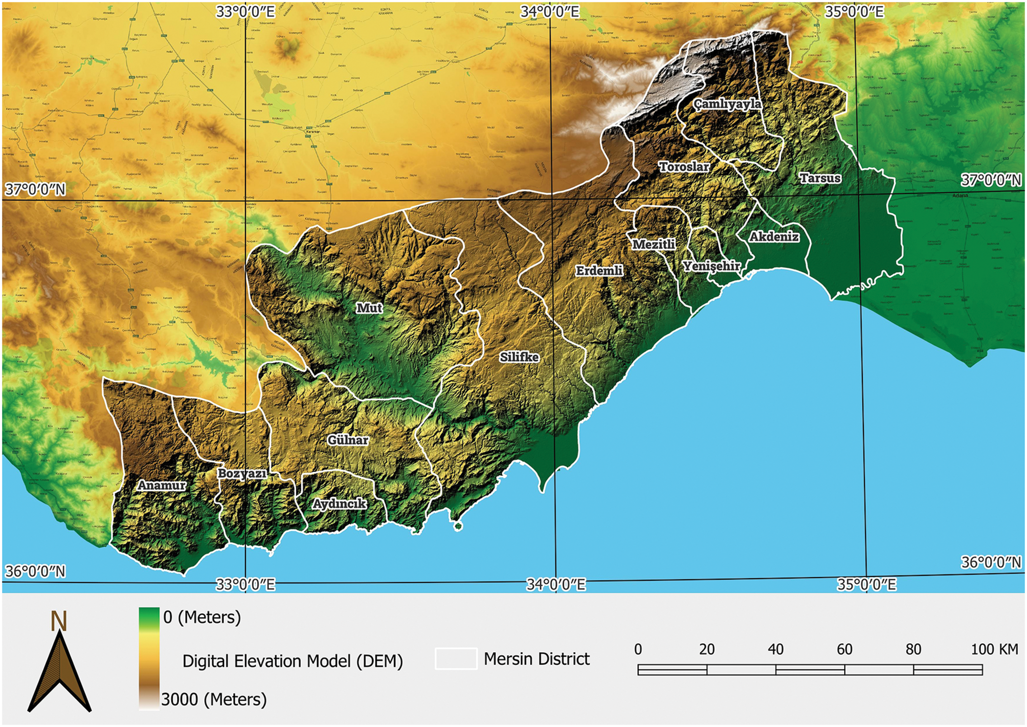
Figure 1: Location of study area

Mersin has a Mediterranean climate with hot and dry summers and mild and rainy winters. The Mediterranean climate classification places Mersin in the arid climate type with an aridity coefficient of 1.02, while the DeMartonne climate classification places it in the semi-arid to humid climate type class with an aridity index value of 10.71 [28]. The average annual precipitation is 615.5 mm, according to the average value of the General Directorate of Meteorology (GDM) between 1940 and 2020. The majority of precipitation occurs in the winter in the form of rain. The average annual temperature is 19.2°C. The highest temperature is 23.4°C, and the lowest is 14.8°C. However, these values change as you move from the coast to higher elevations [29,30]. The average duration of sunshine is 7.5 h, and the average number of rainy days is 79. On 13 January 1950, researchers measured the highest snow thickness at 2 cm. The highest daily precipitation was 199.5 mm on 26 December 1968 [31].

2.2 WorldClim Data

Between 1970 and 2000, high-resolution spatial data was produced worldwide using data from 9000 to 60,000 stations. The project’s scope produced maximum, average, and minimum temperature maps within this data set every month. The data from the stations was processed using interpolation techniques and converted into a raster format [32].

2.3 Calculation of Tourism Climate Index

The tourism climate index (TCI) is used to assess whether climate conditions are favorable for tourism. TCI is calculated by combining two bioclimatic conditions and three climatic elements. The bioclimatic elements are daylight comfort index and daily comfort index. The daylight comfort index is calculated by dividing the temperature values in Fig. 2 by the relative humidity values. The daily comfort index is calculated by dividing the temperature humidity values in Fig. 2. These calculations are applied to each meteorological observation station used in the study. The values calculated at the stations are then generalized for the entire study area using any interpolation technique. Interpolation, shortly, can be defined as the process of estimating the measurement data at any location without actually taking measurements at that location, using a developed mathematical model [33]. The Inverse Distance Weighted (IDW) interpolation method is based on weighting the inverse of the distance between the support points and the point to be predicted. In the IDW method, the aim is to reduce the influence of the distant point on the predicted value as the distance to the support points increases. The formula used today to calculate the tourism climate index was first developed in 1985 to assess climate impact on general tourism activities [10,34]. The TCI’s calculation theory is based on the human body’s physiological response to climate. The TCI incorporates climate variables like effective temperature, rainfall, wind, and solar radiation, all of which are crucial for tourists’ activities [34–37]. This study calculated the TCI to assess the climatic impact of tourism in Mersin Province on human health. Mieczkowski (1985) developed the formula (Eq. (1)) to calculate the TCI [31].

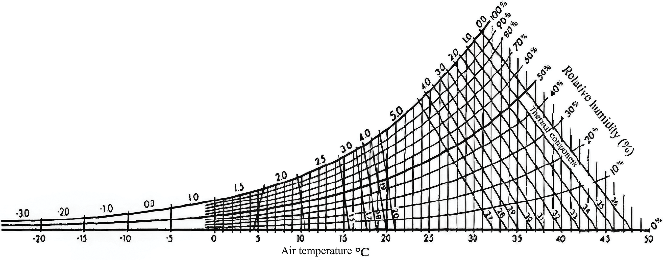
Figure 2: Thermal comfort rating system for TCI [31], Copyright © 1985, Canadian Geographer

(1)

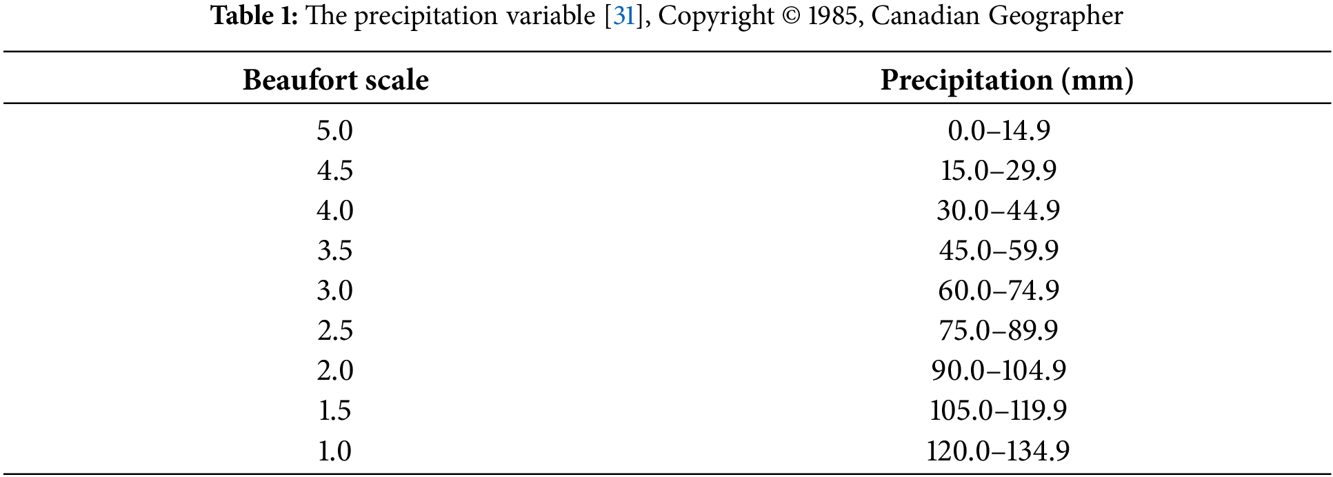
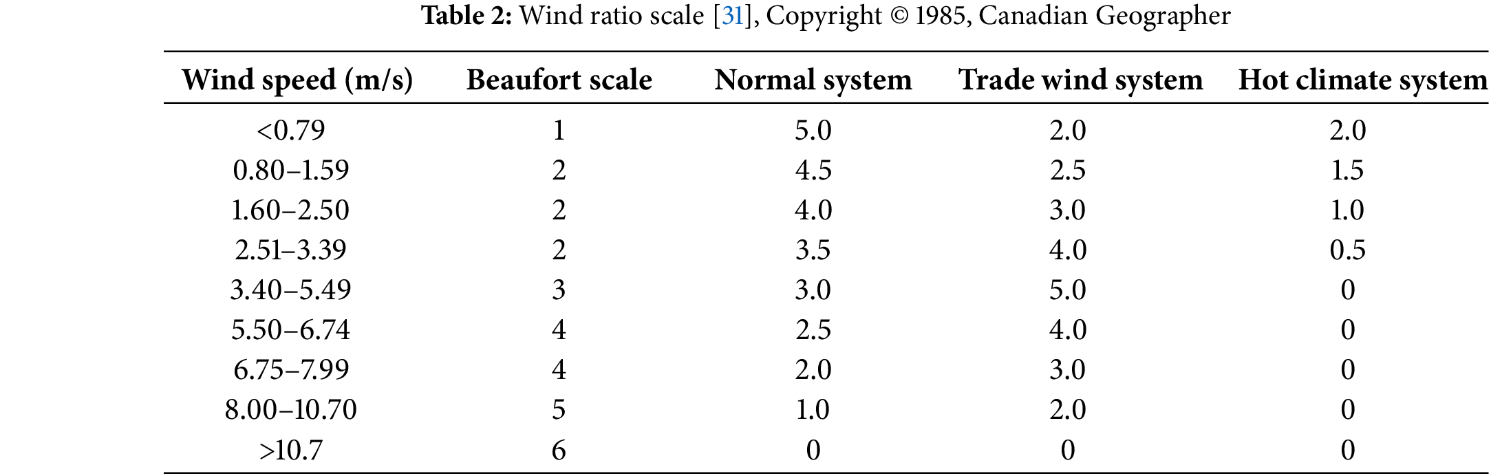
where TCI is tourism climate index, CID is daytime comfort index (determined by maximum daily air temperature in °C and minimum relative humidity in %), CIA is daily comfort index (average daily air temperature in °C and average daily relative humidity in % are used), CID and CIA are calculated based on Fig. 2. R is average monthly rainfall in mm (Table 1). Q is average daily insolation in hours (Table 2). W is average wind speed in m/s or km/h (Table 3).

The formula in Eq. (1) produces the TCI map by multiplying the raster-based maps with the coefficients. The graph in Fig. 2 is utilized to calculate CID and CIA. For each observation, the new value in the bioclimatic comfort rating system is found after the maximum daily air temperature is proportioned to the minimum relative humidity. Interpolation techniques transform these values into a raster-based map, resulting in the production of the CID map. For CIA, average air temperature and relative humidity are proportioned using Fig. 2, and new bioclimatic comfort rating system values are found. The CIA map is then converted into a raster-based map with interpolation techniques, and the CIA map is produced. Tables 1–3 are used during the production of R, S and W maps.

The rainfall values obtained from meteorological observation stations are converted into a new value corresponding to the precipitation value in Table 1. Interpolation techniques transform this value into a raster-based map. This map is substituted in the formula and used to calculate TCI. Examining Table 1 reveals that areas with low rainfall have a high score value, while those with high rainfall have a low score value.

The wind speed values of the meteorological observation stations are converted into the new normal system value corresponding to the wind speed value in Table 2. Interpolation techniques convert these values into a raster-based map. This map is substituted in the formula and used to calculate TCI. Examining Table 2 reveals that the coefficient is low in high wind speed areas and high in low wind speed areas.

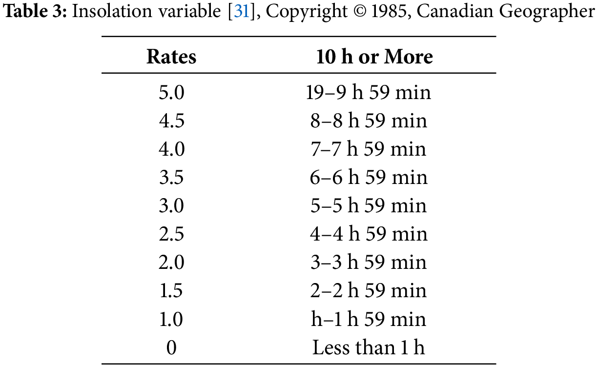
The sunshine duration value obtained from meteorological observation stations is converted into rates corresponding to the 10 H or more value in Table 3. Interpolation techniques transform these values into a raster-based map, which we then substitute in Eq. (1) to calculate TCI. Analysis of Table 3 reveals a linear relationship between the insolation time and the coefficient. If the duration of sunshine is high, the coefficient is high, while if the duration of sunshine is low, the coefficient is low. More sunshine will lead to more daytime tourism activities in the region.

Eq. (1) substitutes the raster-based maps created for TCI calculation, transforms the numerical values into thematic maps based on the code column values in Table 4, and interprets the results according to the climate category for tourism.

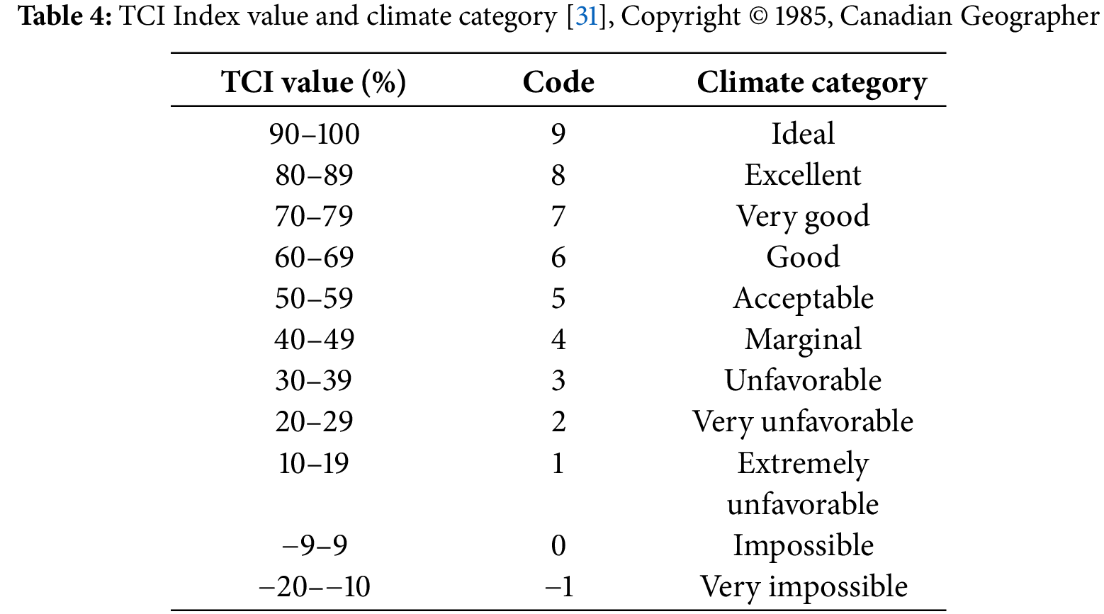
According to the index values, Table 4 analyzes destinations between 60% and 69% as “good” destinations with a climate suitable for tourism.

2.4 Calculation of Heat Index (HI)

In July 1995, more than 700 deaths occurred in Chicago, USA, in an attempt to investigate the relationship between air temperatures and the bioclimatic comfort index [34]. This index examines the relationship between ambient temperature and relative humidity. Studies on the heat index have observed that variations in temperature and relative humidity can influence the felt temperature [35–37]. Eq. (2) [38] provides the formula to calculate the heat index.

(2)

where HI is heat index, T is air temperature (°F), R is relative humidty (%).

A classification is used to evaluate the results of the applied formulas. The classification used in the results evaluation is given below. In evaluating the results obtained from the calculation, the classes given in Table 5 were used for the classes of HI values.

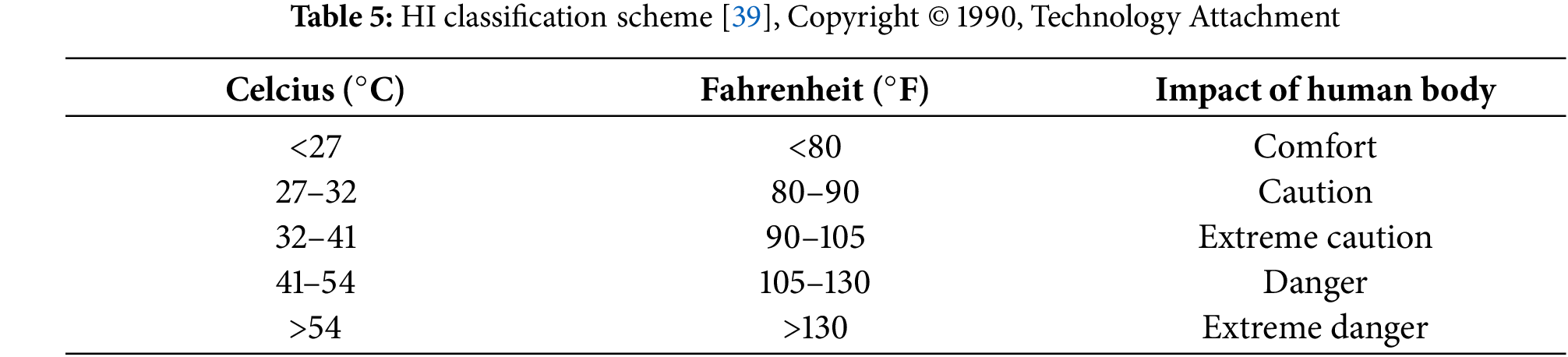
Table 5 reveals that individuals should exercise caution when venturing outdoors at temperatures exceeding 27°C. Hazardous situations may occur, especially when the felt ambient temperature is higher than 54°C. Heat stroke, in particular, may occur in the human body [40].

2.5 New Summer Simmer Index (NSSI) Calculation

The Summer summer index, initially developed by Pepi in 1987 [40] and then developed by different researchers in the following years, is an index that calculates the felt temperature using temperature and humidity based maps. In general, this index is based on scientific principles, verified by independent physiological models, and supported by hundreds of tests on human individuals [41–43]. The most important feature of this index is that the effect of temperature and humidity on the human body is proved by testing. The concerns and discomfort caused by thermal stress on the human body are converted into meaningful equivalent temperature values. During the creation of this index, the existing literature of the past 75 years was analyzed and the deficiencies were removed. The Summer Temperature Index is based on scientific principles, validated by independent physiological models, and supported by hundreds of tests on human subjects. This index translated thermal stress and discomfort concerns into meaningful equivalent temperature values. Existing literature from the past 75 years was reviewed, and gaps were identified. The new summer simmer index (NSSI) was then created. Kansas State University tested and analyzed the results from the work of the American Society of Heating and Refrigerating Engineers (ASHRAE). The SSI is the only temperature-humidity index that uses proven physiological models and human testing results. It can fulfill all subjective and objective requirements for a dry environment. Therefore, people can use it not only as an indicator of their body temperature but also as a clear warning for those at risk of the physiological hazards of heat exposure. Eq. (3) [40] calculates the index.

(3)

where NSSI is new summer simmer index, Ta is air temperature (°F), Ur is relative humidity (%). Table 6 displays the classes of SSI values after the calculation.

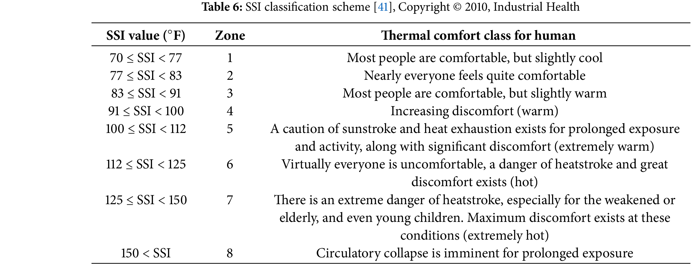
Table 6 shows people’s thermal comfort classes according to the calculated SSI value.

2.6 Model Development in QGIS for Tourism Climate Index

The ModelBuilder tool in QGIS software enables the design of numerous models for various purposes. This tool enables the models to incorporate functions from the plug-ins downloaded into QGIS. This tool enabled the realization of the model design.

Our main input parameters in the model produced for TCI calculation are CID, CIA, P, S, and W in raster format. The values obtained from the ratio of CID and CIA values to the temperature and humidity values in Fig. 2 should be converted into raster format using interpolation techniques. In the exact figure, the parameters P, S, and W should be converted to the class values in Tables 1–3, respectively. Raster maps of these class values should be given as input parameters. In order to output the resulting map of the study area in raster format, it is optional for the user to enter the pixel size and coordinate system information of the raster. The model requests an output area within the polygon structure to obtain the desired area. This way, the user can get the output at the desired pixel size and coordinate system information for the desired area (Fig. 3).

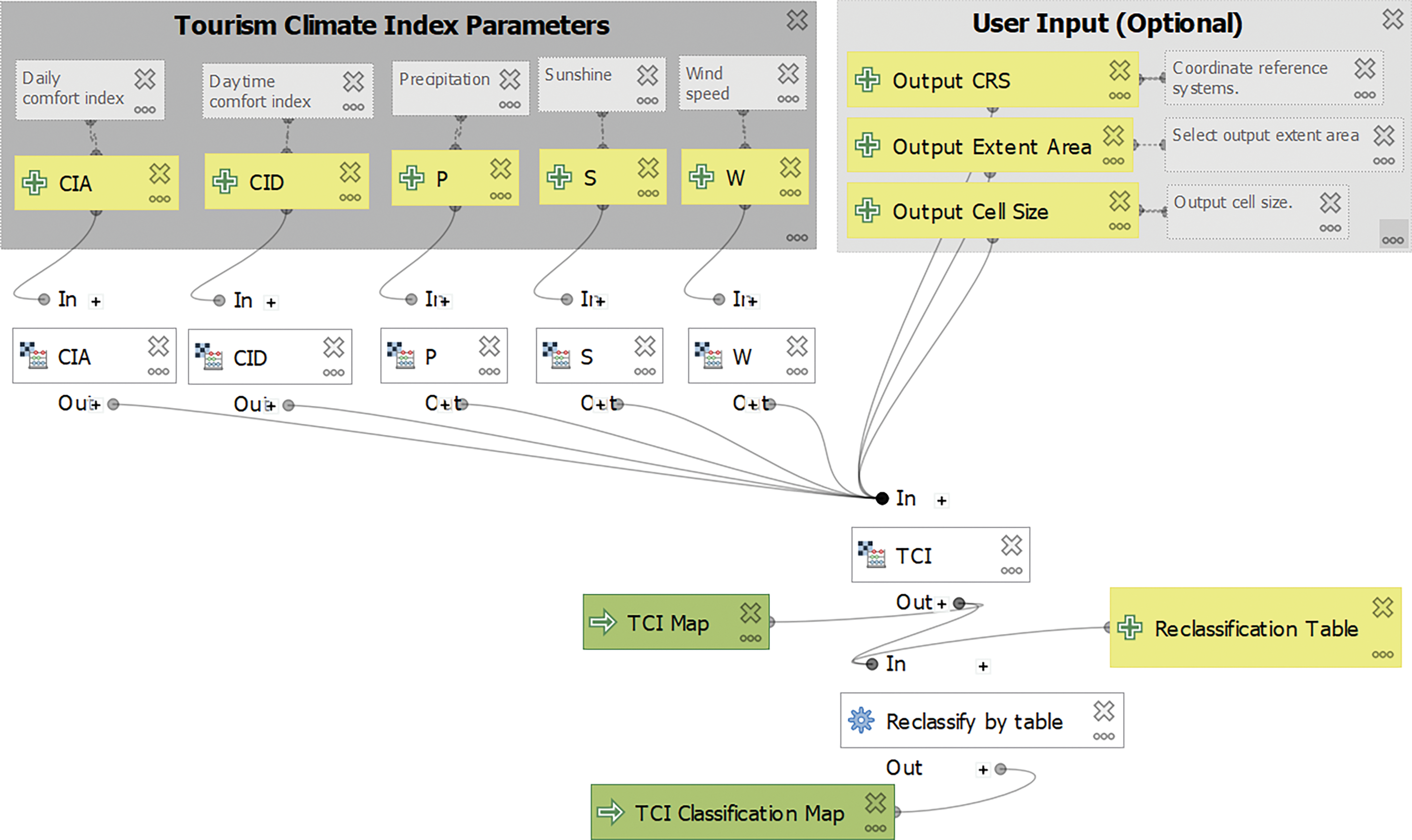
Figure 3: TCI model design

2.7 Model Development in QGIS for Heat Index (HI)

The primary input parameters for HI calculations are raster-format air temperature and relative humidity maps. It is optional to input the raster’s pixel size and coordinate system information to shape the output. However, the output area must be entered as a polygon to produce a map according to an area. Upon completion of the entered information, running the model activates the dialog window. This dialog displays the model’s input parameters, after which the model generates the maps (Fig. 4). Tables 4 and 5 automatically classify the generated maps based on the class values. Users can manipulate these class maps if they wish.

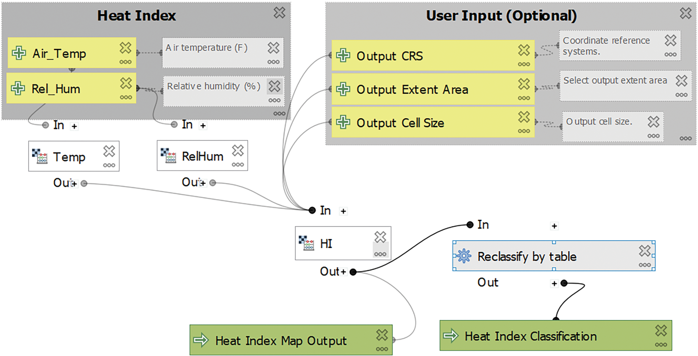
Figure 4: HI model design

2.8 Model Development in QGIS for the New Summer Simmer Index (NSSI)

The American Meteorological Society introduced the SSI, a much more advanced form of comfort indices used to determine bioclimatic comfort conditions for summer tourism, as the “New Millennium Index” at its meeting in Long Beach, California, in July 2000. This index is based on the simultaneous effect of temperature and relative humidity, which was revealed by studies conducted by ASHRAE and confirmed by tests and analyses performed by Kansas State University using the results of physiological models that have been validated for more than 75 years [40–43].

The primary input parameters for the SSI calculation are the air temperature and relative humidity maps in raster format. It is optional to input the raster’s pixel size and coordinate system information to shape the output. However, the output area must be entered as a polygon to produce a map according to an area. After completing the entered information, running both models activates the dialog window. This dialog displays the model’s input parameters, after which the model generates the maps (Fig. 5). Tables 4 and 5 automatically classify the generated maps based on the class values. Users can manipulate these class maps if they wish.

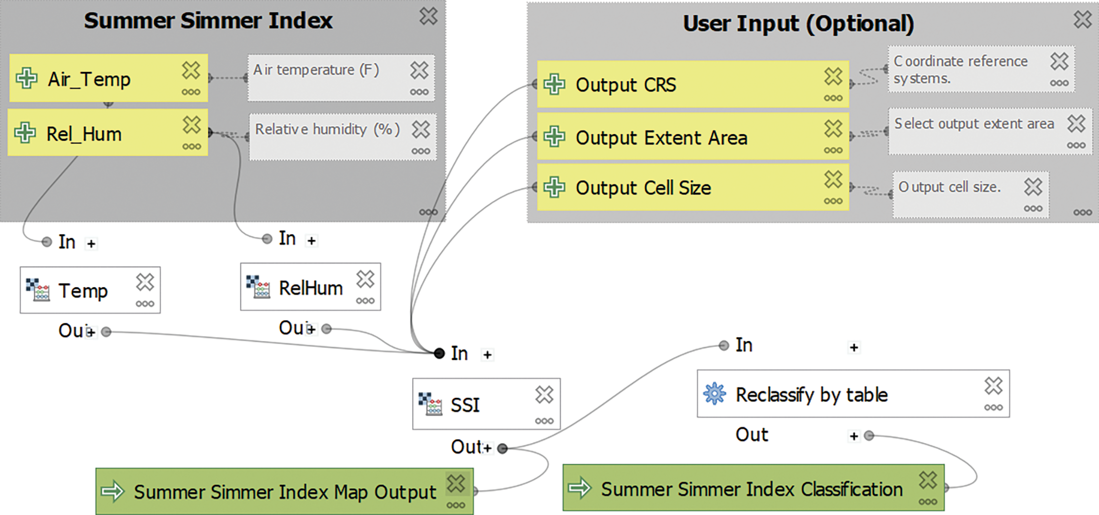
Figure 5: SSI model design

There are two ways to run the created models. The first way is to call the model using the Model Builder tool in QGIS. The algorithm is run with the run model command. The second method involves locating the directory where QGIS stores the production models. The name of this directory is “C:\Users\username\AppData\Roaming\QGIS\QGIS3\profiles\default\processing\models”.

The generated models can be run automatically if placed in this directory. Detailed information about the models and installation is available at https://github.com/efdalkaya/QGIS_Model (accessed on 16 January 2025). Users who want to use the models can download them from GitHub and run them using one of the two methods mentioned above. The Model Builder tool allows users to open models and add desired features.

3  Results

The expectations of scientists conducting research in earth science are evolving due to advancements in computer technology. They are looking for the answer to how to analyze the data obtained most recently. The development of computer technology, especially in recent years, has positively impacted GIS technology. Writers in various programming languages develop new scientific analysis techniques using open-source software. The QGIS software continuously adds new analysis features and numerous add-ons. This study has gained essential features for geoscientists and researchers working on tourism through the design of models. Presenting the developed models to the users also allows different scientists to develop new models by making edits to the plug-in.

Today, one can carry out tourism activities regardless of the time of day. This study modeled three models for evaluating tourism activities in QGIS, making calculations possible without the need to write formulas repeatedly (Fig. 6).

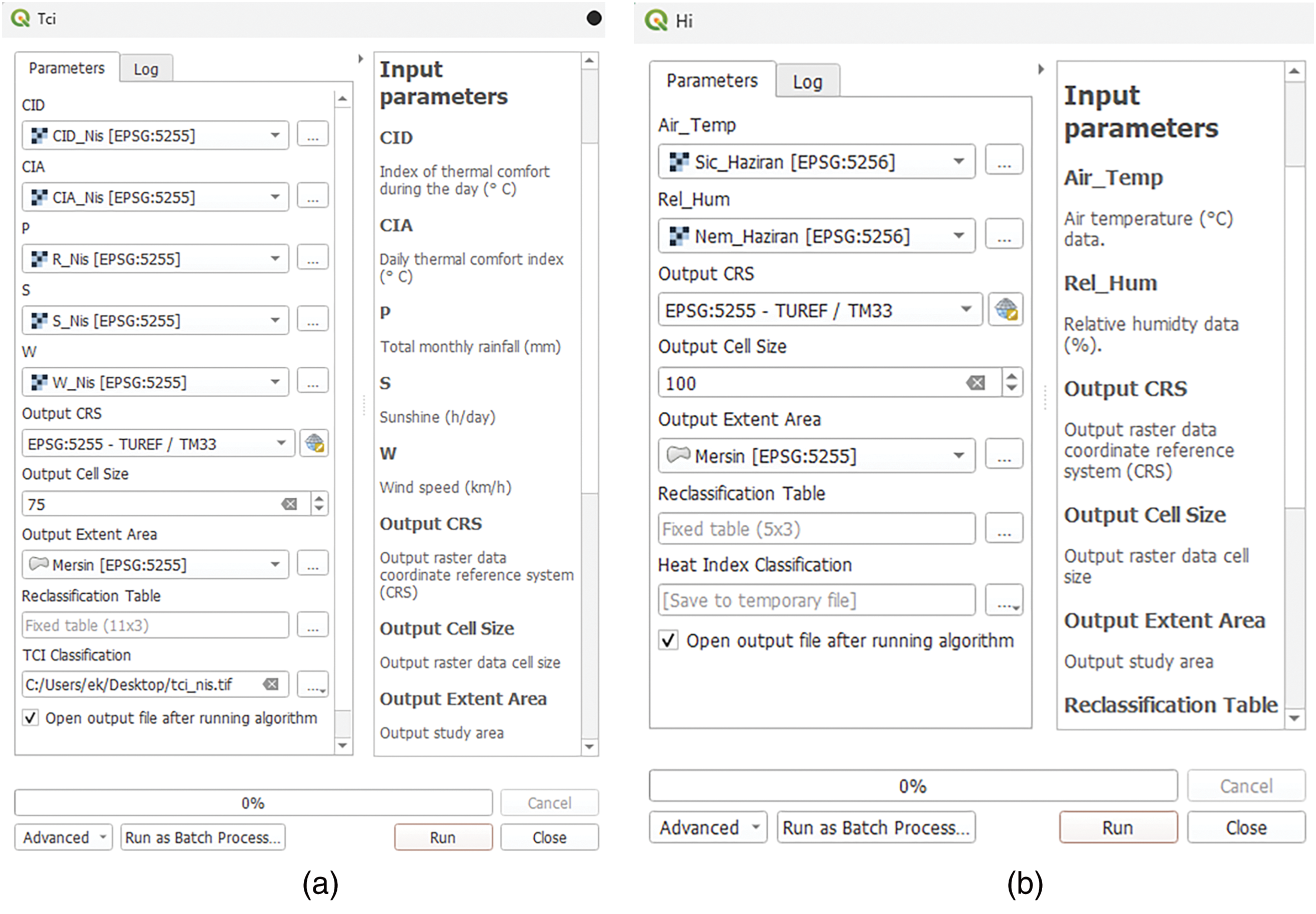
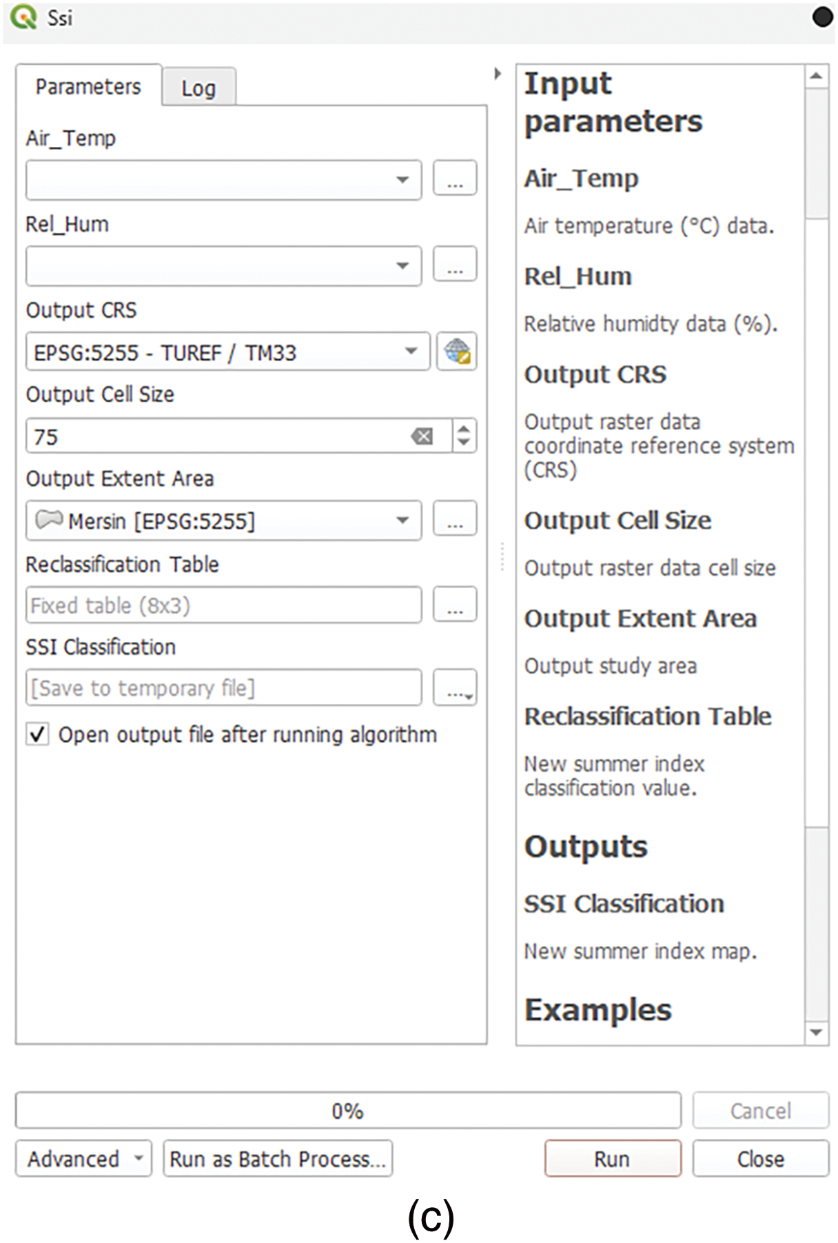
Figure 6: Dialog windows obtained by running (a) TCI, (b) HI and (c) SSI models

4  Discussion

The literature uses licensed and open-source software to calculate bioclimatic comfort indices. Licensed and open-source software cannot directly calculate all bioclimatic comfort indices. Most studies [42–45] have used the Raster Calculator tool in ArcGIS software to calculate TCI, HI, and SSI. Kaya (2023) used QGIS to create a heat index map for Kocaeli Province [46]. He calculated the heat index using the Raster Calculator tool in QGIS. Studies conducted in the literature using licensed software reveal its limitations. One cannot conduct a study using licensed software without purchasing modules. This situation limits scientific studies. However, open-source QGIS software has led to developing unique models and plug-ins for various fields. Nowak et al. (2023) developed a plug-in that supports ecosystem services for agricultural landscapes [47]. With this model’s help, drought’s impact on biodiversity in agricultural areas can be analyzed. Celik (2023) developed an open-source linear spectral separation tool for hyperspectral and multispectral images in the model [48]. For each model developed, there are essential formulas. In the models developed in this study, the formulas used to calculate TCI, HI, and SSI must be carefully written into the Raster Calculator tool in the software each time. A mistake in the formulas can produce different class maps. These models, developed in QGIS, have eliminated this scenario. Open-source software has made an essential contribution by enabling the automatic calculation of climatic models for the first time in the literature. No software can directly calculate these three models, but open-source QGIS software can quickly produce TCI, HI, and SSI maps.

Therefore, three indices developed for evaluating bioclimatic climate conditions for tourism were modeled in QGIS software. Linear regression analysis was performed to investigate the accuracy of the models. The information about the regression produced as a result of the analysis is shown in Fig. 7.

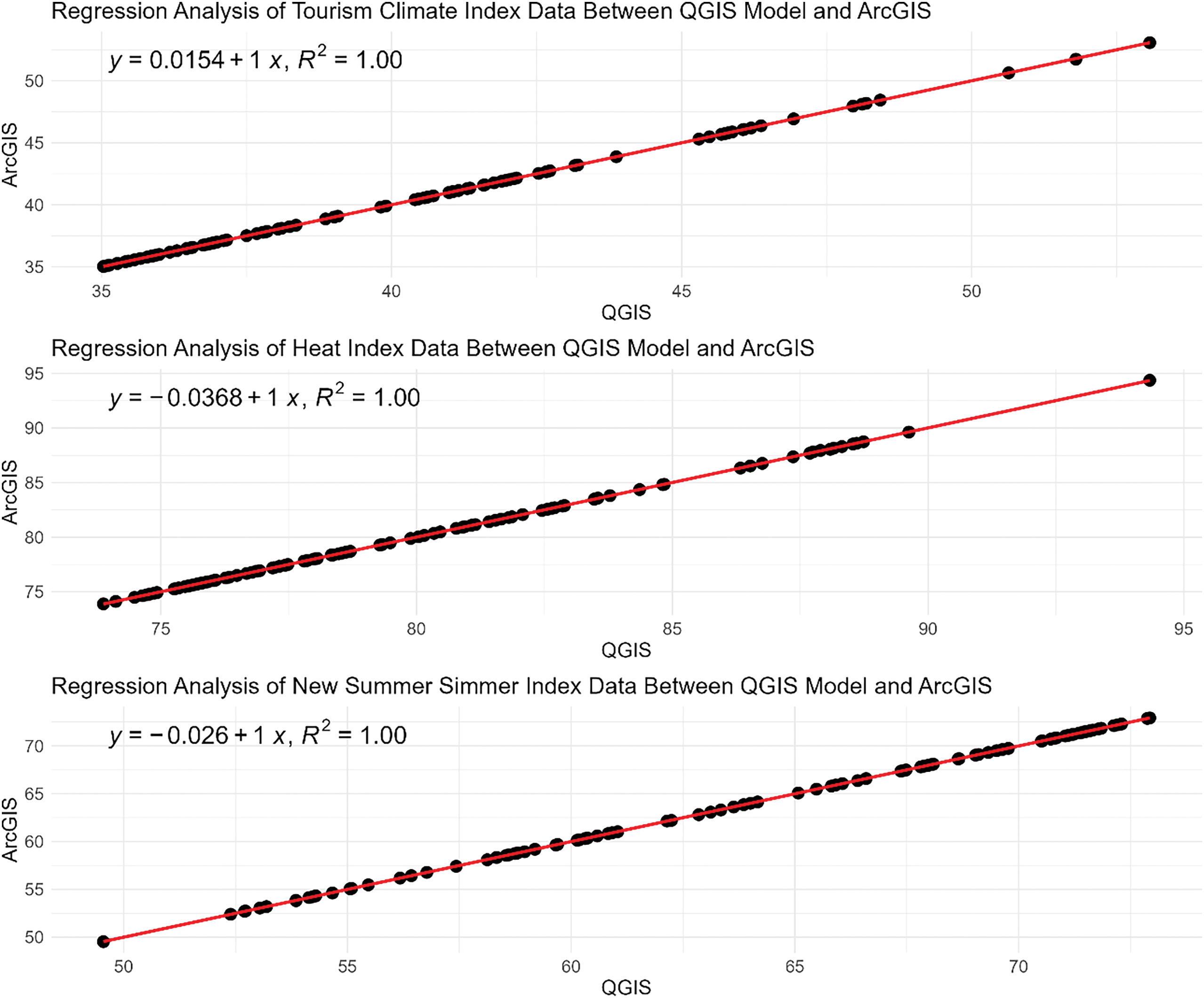
Figure 7: Regression analysis results of different models

Fig. 7 shows the results of the regression analysis between the models produced in QGIS and the models produced in ArcGIS software. As a result of the analyses performed for TCI, HI and SSI, R2 value is 1. The fact that the R2 values of the models produced are 1 directly reveals that the models produced from QGIS software can be used. In order to compare the maps produced as a result of the model, the Raster Calculator tool in ArcGIS was used. Figs. 8–10 show the maps produced in both ways.

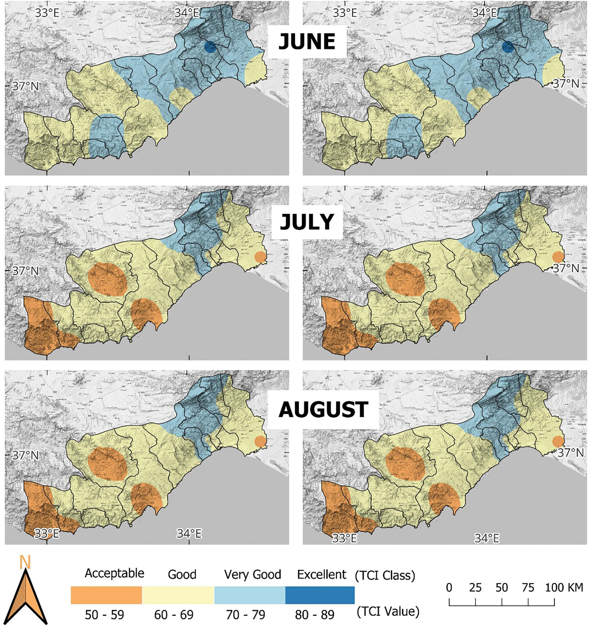
Figure 8: The maps in the left section are the TCI maps produced using ArcGIS, and the maps in the right section are the TCI maps produced by running the model in the QGIS environment

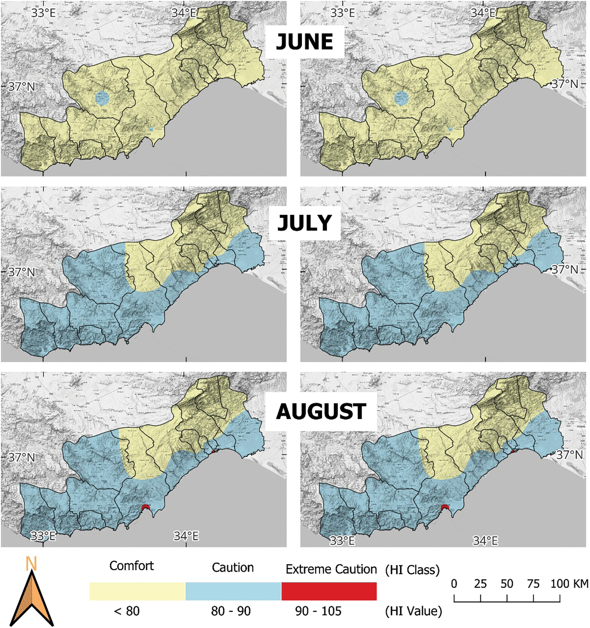
Figure 9: The maps in the left section are the HI maps produced using ArcGIS, and the maps in the right section are the HI maps produced by running the model in the QGIS environment

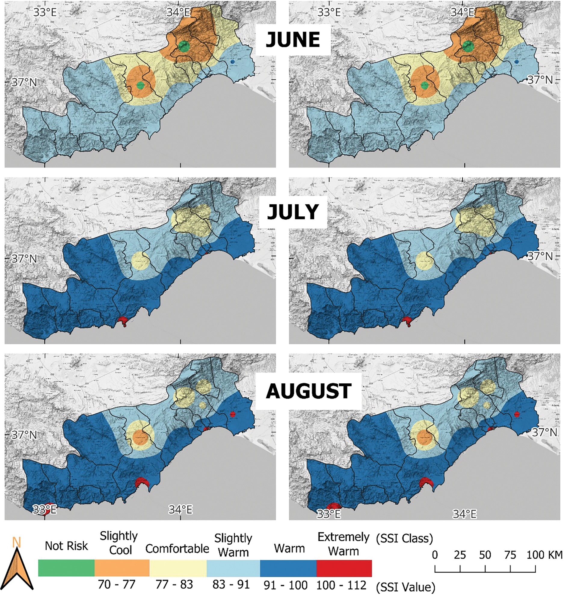
Figure 10: The maps on the left are SSI maps produced using ArcGIS, and the maps on the right are SSI maps produced by running the model in the QGIS environment

Fig. 8 shows the TCI map for Mersin Province. When the TCI classes for June are analyzed, perfect classes are observed in Akdeniz, Çamlıyayla, Tarsus, Toroslar, Yenişehir districts, and the higher parts of Silifke and Mezitli districts. Anamur, Aydıncık, Bozyazı, Gülnar, Mut, and Silifke districts have good environmental conditions for wet tourism activities. Mersin province can efficiently plan outdoor tourism activities in June. Analyzing the TCI class map for July reveals that the outdoor sensible temperature values in Gülnar, Mut, Erdemli, Mezitli, and Yenişehir districts are acceptable. Anamur, Akdeniz, Aydıncık, Bozyazı, Erdemli, Tarsus, and Silifke districts have a suitable outdoor temperature. During the hottest summer months, perfect and excellent weather conditions are observed in Çamlıyayla and the higher parts of Toroslar districts. This month, Taurus and Çamlıyayla districts can plan nature sports tourism activities. In general, all kinds of tourism activities can be planned except for the places where acceptable temperature values are observed. Analyzing the TCI class map for August reveals that only a few parts of Mut and Silifke experience acceptable weather conditions, whereas most districts enjoy excellent outdoor temperatures. Activities for nature tourism can be organized, especially in the higher parts of the Taurus region.

TCI maps determine in which periods of the year the climatic conditions are ideal for touristic activities, and different activities can be organized for tourists in periods with high TCI values. In addition, new tourism destinations can be created for areas with high TCI values, and indoor activities can be created for areas with low TCI values. While indoor activities can be organized in almost all of Mersin Province for June, indoor activities can be organized especially in Mut, Silifke and Taşucu districts for July and August.

Fig. 9 shows the HI map for Mersin Province. Examining the HI classes for June reveals that all districts are climatically comfortable, except a tiny area in Mut district that requires attention to temperature. When the HI classes map for July and August is examined, the areas higher than the sea, especially Çamlıyayla, Erdemli, Mezitli, and Toroslar districts towards the Taurus Mountains, are in the comfortable class, while the temperature should be considered in other districts. One should not stay outdoors too much in these districts when planning tourism activities.

Fig. 10 shows the SSI map for Mersin Province. Examining the SSI class map for June and July reveals that all districts have excellent climatic conditions, except a small area in Mut district in July that falls into the slightly excellent category. When the SSI class map for August is examined, it is seen that Çamlıyayla, Erdemli, Mezitli, and Toroslar districts, which are higher than the sea, especially towards the Taurus Mountains, have slightly cool areas, while almost all other districts are in the comfortable area class. Mut District and parts of Anamur and Silifke districts near the sea have noticeably hot weather. Planning tourism activities should consider these situations.

In addition, SSI maps for tourism facilities also enable the utilization of solar energy systems. The utilization of solar energy systems by tourism facilities will also reduce the carbon footprint of the region. SSI maps allow the establishment of outdoor activities, nature walks and camping areas due to the high sunlight potential. Examining Figs. 8–10 reveals no difference between the maps produced by building the model and those produced using ArcGIS software. It was revealed that the maps produced by running the model can be easily used for various studies. In most of the study area, tourism activities can be carried out without interruption. Only in certain periods, it is necessary to pay attention to the temperature, which is one of the climate parameters, and not to stay too long under the sun.

5  Conclusion and Recommendation

Tourism is one of the most critical sectors that provides economic returns to constantly and rapidly growing countries. Climatic conditions are one of the most important factors affecting tourism activities. Climatic conditions directly affect the bioclimatic comfort of tourists participating in tourism activities according to their activity types. Effective tourism planning relies on determining bioclimatic comfort conditions. The world is facing almost irreversible climate change. This situation will affect every country on the planet. These negative impacts on countries’ climates will cause a decrease in tourism activities in the coming years. Mersin is one of the most critical provinces in Turkiye in terms of tourism. Mersin has a variety of tourism activities in every season. Tourism plans should be created according to the climate change scenarios experienced in this province. Tourism activities should be reorganized by considering bioclimatic climate conditions, and plans should be prepared for the future.

In this study, TCI, HI, and SSI, which are used to assess tourism-oriented climatic conditions, were designed as models in QGIS software. Temperature, humidity, precipitation, wind speed, and sunshine duration were used to calculate TCI. When the maps produced using both the model and ArcGIS software are examined, the TCI classes for Mersin Province in June, July, and August are “acceptable,” “good,” “perfect,” and “excellent.” Temperature and humidity parameters were used for HI. When the HI maps were classified in terms of bioclimatic conditions, “comfort,” “caution,” and “extreme caution” were found. Especially in July and August, it is essential for people’s health not to do outdoor activities during the daytime in the center of Mersin and Taşucu districts. Temperature and humidity parameters were used for SSI. Bioclimatic conditions classified the SSI maps into “slightly cool,” “comfortable,” “slightly warm,” “warm,” and “extremely warm.” According to the class map, people should not stay outside for too long in July and August for outdoor tourism activities in Anamur Center, Mersin Center, Tarsus Center, and Taşucu Center. Climatic conditions may cause health problems. June has favorable climatic conditions for tourism activities in Mersin. Plan tourism activities in mountainous areas away from city centers in July and August. Overall evaluation of the study results reveals that Mersin Province can plan various outdoor activities for the summer season. However, some city centers should plan long-stay outdoor tourism activities in July and August. It is more climatically appropriate to plan tourism activities at higher elevations. Mersin Province can enhance its tourism potential by offering various activities throughout the summer.

This study not only designed a model to evaluate tourism activities in Mersin but also went beyond that. These models, developed in QGIS to predict tourism demand changes due to climate change, can be applied to various regions for effective planning. Climate change can cause extreme weather events, changing temperature conditions and local microclimatic changes. In this context, bioclimatic maps produced with QGIS support the adaptation of the site to climate change. In addition, with QGIS, risk mapping in the context of bioclimatic comfort and accurate resource management can be carried out through decision support tools. Risk analyses can be conducted based on tourism climate indices by utilizing various datasets in the tourism sector. According to the results of these analyses, forecasts and predictions can be made to determine future tourism activities. Due to the software’s open-source nature, QGIS software allows for rapidly developing versatile models, facilitating accurate predictions and forecasts. The study aims to develop new models and plug-ins in later stages to precisely calculate additional bioclimatic comfort indices. These models and plug-ins are anticipated to support various studies across professional fields by offering accessibility to diverse disciplines. In this manner, researchers from various backgrounds can collectively contribute to the scientific community by adapting the models to their research. The results of this article will aid in advancing new research focused on assessing the impacts of climate change on tourism through the utilization of QGIS software. Using web-based applications to present analysis results can serve as a valuable guide for users and stakeholders in the tourism sector. In addition, this study is planned to be converted into an extension that allows more climate models to be calculated in the future.

Acknowledgement: The author would like to thank the editors and reviewers for their review and recommendations.

Funding Statement: The author received no specific funding for this study.

Availability of Data and Materials: The author confirms that the data supporting the findings of this study are available within the article.

Ethics Approval: Not applicable.

Conflicts of Interest: The author declares no conflicts of interest to report regarding the present study.

References

1. Arıca F, Kaya B. COVID-19 Pandemisi ve Türk Turizm Sektörü Üzerindeki Etkisi. Polit Ekon Kuram. 2022;6(1):102–18 (In Turkish). doi:10.30586/pek.1079267. [Google Scholar] [CrossRef]

2. Curtale R, e Silva FB, Proietti P, Barranco R. Impact of COVID-19 on tourism demand in European regions—an analysis of the factors affecting loss in number of guest nights. Ann Tour Res Empir Insights. 2023;4(2):100112. doi:10.1016/j.annale.2023.100112. [Google Scholar] [CrossRef]

3. Henseler M, Maisonnave H, Maskaeva A. Economic impacts of COVID-19 on the tourism sector in Tanzania. Ann Tour Res Empir Insights. 2022;3(1):100042. doi:10.1016/j.annale.2022.100042. [Google Scholar] [CrossRef]

4. Hu Y, Lang C, Corbet S, Wang J. The impact of COVID-19 on the volatility connectedness of the Chinese tourism sector. Res Int Bus Financ. 2024;68:102192. doi:10.1016/j.ribaf.2023.102192. [Google Scholar] [CrossRef]

5. WMO. Economic costs of weather-related disasters soars but early warnings save lives; 2023 [cited 2023 Oct 15]. Available from: https://wmo.int/media/news/economic-costs-of-weather-related-disasters-soars-early-warnings-save-lives. [Google Scholar]

6. World Health Organizations. Climate change; 2023 [cited 2023 Oct 20]. Available from: https://www.who.int/health-topics/climate-change#tab=tab_1. [Google Scholar]

7. Gökalp Kutlu A. Incorporating climate change into the women, peace, and security Agenda. Altern Polit. 2024;16(1):31–61. doi:10.53376/ap.2024.02. [Google Scholar] [CrossRef]

8. Ghalhari GF, Heidari H, Dehghan SF, Asghari M. Consistency assessment between summer simmer index and other heat stress indices (WBGT and Humidex) in Iran’s climates. Urban Clim. 2022;43:101178. doi:10.1016/j.uclim.2022.101178. [Google Scholar] [CrossRef]

9. Rosselló-Nadal J. How to evaluate the effects of climate change on tourism. Tour Manage. 2014;42:334–40. doi:10.1016/j.tourman.2013.11.006. [Google Scholar] [CrossRef]

10. Wang H, You Q, Liu G, Wu F. Climatology and trend of tourism climate index over China during 1979–2020. Atmos Res. 2022;277:106321. doi:10.1016/j.atmosres.2022.106321. [Google Scholar] [CrossRef]

11. Olya HGT, Alipour H. Risk assessment of precipitation and the tourism climate index. Tour Manage. 2015;50:73–80. doi:10.1016/j.tourman.2015.01.010. [Google Scholar] [CrossRef]

12. Tecim V. Coğrafi Bilgi Sistemleri: Harita Tabanlı Bilgi Yönetimi. Ankara, Turkyie: Renk Form Ofset Matbaacılık Ltd. Şti; 2008. 363 p (In Turkish). [Google Scholar]

13. Önder YE, Kavzoğlu T. Açık Kaynak Kodlu CBS Yazılımları ile Trafik Kaza Yoğunluk Analizleri: İstanbul Örneği. Türkiye Coğrafi Bilgi Sist Derg. 2020;2(1):1–9 (In Turkish). [Google Scholar]

14. Kotan B, Erener A. Seasonal analysis and mapping of air pollution (PM10 and SO2) during COVID-19 lockdown in Kocaeli (Türkiye). Int J Eng Geosci. 2023;8(2):173–87. doi:10.26833/ijeg.1111699. [Google Scholar] [CrossRef]

15. Çolak E, Bediroğlu G, Memişoğlu Baykal T. GIS-based determination of potential snow avalanche areas: a case study of rize province of Türkiye. Int J Eng Geosci. 2024;9(2):199–210. doi:10.26833/ijeg.1367334. [Google Scholar] [CrossRef]

16. Ajaj QM, Shafri HZM, Wayayok A, Ramli MF. Assessing the impact of Kirkuk cement plant emissions on land cover by modelling Gaussian plume with Python and QGIS. Egypt J Remote Sens Space Sci. 2023;26:1–16. doi:10.1016/j.ejrs.2022.12.001. [Google Scholar] [CrossRef]

17. Nielsen A, Bolding K, Hu F, Trolle D. An open source QGIS-based workflow for model application and experimentation with aquatic ecosystems. Environ Model Softw. 2017;95:358–64. doi:10.1016/j.envsoft.2017.06.032. [Google Scholar] [CrossRef]

18. Meyer D, Riechert R. Open source QGIS toolkit for the advanced research WRF modelling system. Environ Model Softw. 2019;112:166–78. doi:10.1016/j.envsoft.2018.10.018. [Google Scholar] [CrossRef]

19. Molina-Navarro E, Nielsen A, Trolle D. A QGIS plugin to tailor SWAT watershed delineations to lake and reservoir waterbodies. Environ Model Softw. 2018;108:67–71. doi:10.1016/j.envsoft.2018.07.003. [Google Scholar] [CrossRef]

20. Renard F, Mora V, Horgue P, Kerloch JM. THYRSIS: a QGIS plugin for hydrogeological modelling. Comput Geosci. 2024;187:105580. doi:10.1016/j.cageo.2024.105580. [Google Scholar] [CrossRef]

21. Raimondi L, Pepe G, Firpo M, Calcaterra D, Cevasco A. An open-source and QGIS-integrated physically based model for Spatial Prediction of Rainfall-Induced Shallow Landslides (SPRIn-SL). Environ Model Softw. 2023;160:105587. doi:10.1016/j.envsoft.2022.105587. [Google Scholar] [CrossRef]

22. Al-Thuwaynee OF, Melillo M, Gariano SL, Park HJ, Kim S, Lombardo L, et al. DEWS: a QGIS tool pack for the automatic selection of reference rain gauges for landslide-triggering rainfall thresholds. Environ Model Softw. 2023;162:105657. doi:10.1016/j.envsoft.2023.105657. [Google Scholar] [CrossRef]

23. Adiguzel F. Calculating the tourism climate index for urban planning: a case study of Mersin Province. J Gastron Hosp Travel. 2023;6(3):1253–66. doi:10.33083/joghat.2023.334. [Google Scholar] [CrossRef]

24. Topuz M, Karabulut M. İçel’in iklimi değişiyor mu? Genel bir değerlendirme. İçel Derg. 2022;2(1):18–26. [Google Scholar]

25. The information promotion division, real estate and construction economy Bureau. Ministry of Land, Infrastructure, Transport and Tourism; 2022 [cited 2025 Jan 10]. Available from: https://github.com/jinryuhudojyouhoukatsuyou/people_flow_visualization. [Google Scholar]

26. Wilkinson T, Petersen C, Bell A, Bearman N, Barbier L. GIS mapping and modelling of tourism pressure and opportunities for sustainable tourism in four UNESCO biosphere reserves (UK and Francea decision-support tool to guide strategic tourism decision-making. Centre for Rural Policy Research (CRPRUniversity of Exeter: BioCultural Heritage Tourism Project Report; 2021 [cited 2025 Jan 10]. Available from: https://github.com/mopst/reports. [Google Scholar]

27. Bilici ÖE, Everest A. 29 Aralık 2016 Mersin selinin meteorolojik analizi ve iklim değişikliği bağlantısı. Doğu Coğrafya Derg. 2017;22(38):227–50 (In Turkish). doi:10.17295/ataunidcd.294027. [Google Scholar] [CrossRef]

28. Karabulut M, Sandal EK, Gürbüz M. 20 Kasım-9 Aralık 2001 Mersin Sel Felaketleri: meteorolojik ve Hidrolojik Açıdan Bir İnceleme. KSU J Sci Eng. 2007;10(1):13–24. [Google Scholar]

29. MGM. Climate Classification: Mersin City. 2024 [cited 2024 May 04]. Available from: https://www.mgm.gov.tr/iklim/iklim-siniflandirmalari.aspx?m=MERSIN. [Google Scholar]

30. Fick SE, Hijmans RJ. WorldClim 2: new 1 km spatial resolution climate surfaces for global land areas. Int J Climatol. 2017;37(12):4302–15. doi:10.1002/joc.5086. [Google Scholar] [CrossRef]

31. Mieczkowski Z. The tourism climatic index: a method of evaluating world climates for tourism. Can Geogr/Le Géographe Can. 1985;29(3):220–33. doi:10.1111/j.1541-0064.1985.tb00365.x. [Google Scholar] [CrossRef]

32. Gao C, Liu J, Zhang S, Zhu H, Zhang X. The Coastal Tourism Climate Index (CTCIdevelopment, validation, and application for chinese coastal cities. Sustainability. 2022;14(3):1425. doi:10.3390/su14031425. [Google Scholar] [CrossRef]

33. Yu D, Li S, Zhang L. Evaluate tourism climate using modified holiday climate index in China. Tour Tribune. 2021;36(5):14–28 (In Chinese). doi:10.3390/atmos6020183. [Google Scholar] [CrossRef]

34. Zhong LS, Yu H, Zeng Y. Impact of climate change on Tibet tourism based on tourism climate index. J Geogr Sci. 2019;29(12):2085–100. doi:10.1007/s11442-019-1706-y. [Google Scholar] [CrossRef]

35. Semenza JC, Rubin CH, Falter KH, Selanikio JD, Flanders WD, Howe HL, et al. Related deaths during the, heat wave in Chicago. N Engl J Med. 1996;335:89–90. doi:10.1056/NEJM199607113350203. [Google Scholar] [CrossRef]

36. Steadman RG. The assessment of sultriness. Part I. A temperature-humidity index based on human phys-iology and clothing science. J Appl Meteorol. 1979;18(7):861–73. doi:10.1175/1520-0450(1979)018<0861:TAOSPI>2.0.CO;2. [Google Scholar] [CrossRef]

37. Steadman RG. A universal scale of apparent temperature. J Clim Appl Meteorol. 1984;23(12):1674–87. doi:10.1175/1520-0450(1984)023<1674:AUSOAT>2.0.CO;2. [Google Scholar] [CrossRef]

38. Zahid M, Rasul G. Rise in summer heat index over Pakistan. Pak J Meteorol. 2010;6(12):85–96. doi:10.4236/jamp.2017.58127. [Google Scholar] [CrossRef]

39. Rothfusz LP. The heat index equation (or, more than you ever wanted to know about heat index). Technology Attachment, SR/SSD 90–23. Forth Worth, TX, USA: NWS Southern Region Headquarters; 1990. [Google Scholar]

40. Pepi JW. New Summer Simmer Index—A Comfort Index for the New Millennium. 1999 [cited 2024 Apr 21]. Available from: http://summersimmer.com/ssi_page5.htm. [Google Scholar]

41. Tzenkova A, Ivancheva J, Koleva E, Videnov P. The human comfort conditions at Bulgarian Black Sea side. Dev Tour Climatol. 2007;150:157. [Google Scholar]

42. Alfano FRDA, Palella BI, Riccio G. Thermal environment assessment reliability using temperature—humidity indices. Ind Health. 2011;49(1):95–106. doi:10.2486/indhealth.MS1097. [Google Scholar] [PubMed] [CrossRef]

43. Morcotet D. The thermal comfort in the surface public transport from bucharest during the summer period. Aerul Si Apa Compon Ale Mediu. 2012;2012:367–74. doi:10.1016/j.scitotenv.2016.05.047. [Google Scholar] [CrossRef]

44. Asghari M, Fallah Ghalhari GA, Heidari H. Investigation of thermal comfort changes using Summer Simmer Index (SSIa case study in different climates of Iran. Open Environ Res J. 2021;14(1):13–23. doi:10.2174/2590277602114010013. [Google Scholar] [CrossRef]

45. Adiguzel F. Effects of green spaces on microclimate in sustainable urban planning. Int J Environ Geoinform. 2023;10(3):124–31. doi:10.30897/ijegeo.1342287. [Google Scholar] [CrossRef]

46. Kaya E. Evaluation of bioclimatic comfort area with heat index: a case study of Kocaeli. Int J Eng Geosci. 2023;8(1):19–25. doi:10.26833/ijeg.988452. [Google Scholar] [CrossRef]

47. Nowak MM, Skowroński J, Słupecka K, Nowosad J. Introducing tree belt designer—a QGIS plugin for designing agroforestry systems in terms of potential insolation. Ecol Inform. 2023;75:102012. doi:10.1016/j.ecoinf.2023.102012. [Google Scholar] [CrossRef]

48. Celik B. QLSU (QGIS Linear Spectral Unmixing) Plugin: an open source linear spectral unmixing tool for hyperspectral & multispectral remote sensing imagery. Environ Model Softw. 2023;168:105782. doi:10.1016/j.envsoft.2023.105782. [Google Scholar] [CrossRef]