Fuzzy Machine Learning-Based Algorithms for Mapping Cumin and Fennel Spices Crop Fields Using Sentinel-2 Satellite Data

1  Introduction

The herb Cuminum cyminum, a member of the parsley family, produces dry seeds known as cumin. An important Rabi crop is cumin, which is generally sown from September to November and harvested from February to April [1]. It has a 100–120-day growth season. The temperature ranges between 25°C and 30°C are ideal for growth. The cumin plant is hand-harvested when it reaches a height of 30–50 cm (12–20 in). Approximately 70% of the world’s cumin production comes from India. In the fiscal year 2020–2021, India produced 856,000 tons of cumin seeds. They are frequently employed in conventional medicine to treat a wide range of illnesses. It is primarily farmed in Rajasthan and Gujarat in India, with 66% and 18% of the country’s total production, respectively [2,3]. Fennel (Foeniculum vulgare L.) is a plant farmed mostly as a herb or for its fruits and admired for its pleasant aroma, multiplicity of nutritional and health characteristics [4]. An important Rabi crop is fennel, which is generally sown from September to November and harvested from February to April. In 180 days, the crop will be ready for harvest [5]. India is the world’s leading producer of fennel. Rajasthan, Andhra Pradesh, Punjab, Uttar Pradesh, Gujarat, Madhya Pradesh, Karnataka, and Haryana are major fennel-growing states.

Remote sensing (RS) data and methods, with the combination of GIS and landscape measures, are essential for the characterization and analysis of Land Cover (LC) spatial and temporal changes [6–8]. Multi-temporal RS datasets allow for the mapping and identification of landscape changes, helping in better landscape management and planning. High and medium-resolution satellite data that are multispectral and multitemporal have become essential resources for quantifying factors like vegetation cover, forest degradation, and urban growth [9]. Information on the dynamics of land cover is analyzed using temporal satellite data. This information can be extracted at a different class level using high-resolution data. Temporal data is helpful to determine the seasonal trend in a particular plant class in addition to spectral data with other classes [10] mentioned that technology for remote sensing and geographic information systems (GIS) offers a platform for investigating from which the Earth’s surface landscapes are covered.

Temporal remote sensing data was applied to map individual crops and collect agricultural growth information [11–13] mentioned that our world’s ecosystem primarily relies on vegetation, which controls the dynamics and productivity of the land cover. Cropping patterns, typical vegetable varieties, and phenology of the target plant can all be determined using time-series vegetation indices suggested by [14].

Mainly three types of classification techniques occurred: supervised, unsupervised, and hybrid classification. In several classifications, the terms ‘hard’ and ‘soft’ are applied. Satellite images are composed of mixed pixels, making classification techniques difficult to apply and producing incorrect results [15]. To address the mixed pixel problem, fuzzy-based classifications were developed, allowing pixels to belong to multiple classes with varying degrees of membership. In addition to this, other techniques such as spectral unmixing and Subpixel Inference Algorithms (SPIA) [16] have been employed. Spectral unmixing decomposes a pixel’s spectral signature into constituent endmember spectra and their abundances, while SPIA uses statistical and machine learning methods to infer the subpixel compositions [17]. These methods, along with fuzzy-based classifications [18], provide robust solutions for handling the complexities of mixed pixels in remote sensing. To deal with the mixed pixel, in this work fuzzy-based classifications were used. In the case of a mixed pixel situation, when it permits membership value to any pixel consisting of the available class, the fuzzy logic technique produces a better outcome. The most extensively used basic fuzzy algorithms in soft classification are FCM [19], PCM [20], and NC [21]. The FCM clustering technique allocates a sample’s membership degree to two or more clusters. PCM uses “degree of belongings” instead of “degree of sharing” to eliminate and smooth out the noise caused by outliers which gives a better result compared to the FCM classifier. To minimize the effect of outliers, the noise clustering technique introduced a distinct class that comprises all of the noisy points. Individual sample as mean is a strategy in fuzzy-based classification that improves classification accuracy while utilizing heterogeneity within the class [22,23].

This research used an innovative approach called “Individual Sample as Mean”, where each training sample is used as the mean parameter for the fuzzy PCM, NC classifier, instead of the conventional statistical mean derived from the training data [24]. The statistical parameters from the training data often fail to represent the variations within a field accurately. Factors such as uneven application of water, fertilizers, and pesticides can cause local variations within a crop field. This heterogeneity negatively impacts classification accuracy and hinders precise crop mapping [23]. So, this study focused on providing the best training sample selection technique to get the best-classified result.

In this study, the cumin and fennel crops were mapped and classified using two methods: the NC and PCM classifiers. There are two distinct ways to choose training samples: “individual training sample as mean” and training sample as “mean”. Individual training samples applied as the mean are a novel methodology, but training samples applied as the “mean” are a traditional method. In this study, the two training sample techniques, “mean” and “individual sample as mean”, applied to NC and PCM classifiers on two temporal indices databases have been compared to see which is more efficient. To reduce the spectral dimensionality of temporal images, the Class-Based Sensor Independent-Modified Soil Adjusted Vegetation Index 2 (CBSI-MSAVI-2) [24] and Modified Soil Adjusted Vegetation Index 2 (MSAVI-2) [25] temporal database indices were used. The temporal vegetation indices were used to consider the various phases of the plant’s crop cycle. By providing details on temporal stage differences from other crops, these indices enhance biophysical quality and provide the target crop with a unique signature. The indices also reduced the albedo/shadow effect in images. The overall objective was to compare the “mean” approach with the “individual sample as mean” training parameter strategy in PCM and NC classifiers, handle heterogeneity within the class, and finally map the cumin and fennel crop. To compare the outcomes, Root Mean Square Error (RMSE), Mean Membership Difference (MMD), Variance, and (Sum of Square Error) SSE were computed. Here, MMD uses two separate approaches to computing. The initial technique uses identical cumin and fennel training and testing samples. The first approach uses the same crop sample as the training and testing samples to determine proximity. The second approach uses the different crop samples as the training and testing samples to determine departure.

2  Detailed Mathematical Explanations of Fuzzy Classifiers

This section discusses the mathematical definitions for the fuzzy machine learning models used in this research work. The fuzzy machine learning Possibilistic c-Mean (PCM) and Noise Clustering (NC) models were used in this analysis. Due to their ability to map just one class of interest, Possibilistic c-Mean (PCM) and Noise Clustering (NC) fuzzy classifiers were chosen.

2.1 Possibilistic c-Means (PCM)

The Possibilistic c-Mean (PCM) algorithm minimizes the constraint of the FCM clustering technique [26]. The hyper-line constraint of the FCM algorithm is simplified by this PCM approach. In contrast to low membership values, which are unrepresentative, the PCM method assigns high membership values to representative factor points. The objective function of the PCM classifier is stated in Eq. (1).

Jm=∑i=1C∑j=1Nujim‖xj−ci‖2+∑i=1Cηi∑j=1N(1−uji)m(1)

ηi=∑j=1Nujim‖xj−ci‖2∑i=1Nuijm(2)

uji=[∑i=1c{‖xj−ci‖ηi}2m−1]−1(3)

Here, ηi = parameter that depends on the distribution of pixels in the cluster in Eq. (2), m = Fuzziness factor (it contains any real value greater than 1), uji = Degree of membership represents of ith pixel for cluster j, xj = jth d-dimensional measured data, ci = mean value (cluster center) of the ith class, ci = mean value (cluster center) of the ith class, N = total no of a pixel in the image, c = Number of classes, and ‖xj−ci‖ = distance between xj and ci.

2.2 Noise Clustering

To deal with the noise, Reference [21] recommended a noise clustering classifier. According to the NC approach, all noise and outliers are included in a new, distinct class. The NC algorithm’s primary function is represented by Eq. (4).

Jm=∑j=1N∑i=1Cujim‖xj−ci‖2+∑j=1Nδ2(1−∑i=1Cuji)m(4)

The membership value Eq. (5) and fuzzy mean Eq. (6) can be derived from the Eq. (4):

uji=1∑k=1c⁡[xi−vj2xi−vk2]1m−1+[xi−vj2δ2]1m−1(5)

νj=∑j=1N(uji)mxi∑j=1N(uji)m(6)

δ2=λ[∑i=1C−1∑j=1N‖xj−ci‖2n(c−1)](7)

‖xj−ck‖ = distance between xj and ck, and δ = noise distance.

2.3 “Individual Sample as Mean” Training Approach

2.3.1 Steps for “Individual Sample as Mean”

The steps followed for the “individual sample as mean” training approach are as follows:

Step 1: n Training samples for each class were selected for both techniques. Here n represent the no. of training sample.

Step 2: The values of the selected training samples were utilized to change the mean values (ci) in the calculation of the membership value for the PCM and NC classifier algorithms. Eqs. (1) and (4), respectively, substitute n for each training sample in PCM and NC.

Step 3: Determined the membership value for each pixel for each training sample for a specific class.

Step 4: Each pixel for each sample within the class is given the membership value with the highest degree.

2.3.2 Utility of Both Training Sample Techniques

Individual training sample as “mean”

1. Dimensionality Reduction: Simplifies the data by reducing the number of features [27].

2. Pattern Discovery: This may help in discovering underlying patterns in the data that could be useful for the model [24].

Training sample as “mean”

1. Consistency: Ensures that the imputation is based on the distribution of the training data, which is crucial to prevent data leakage from the test set [28].

2. Simplicity: Easy to implement and understand, quickly dealing with missing data without introducing complex models.

3. Baseline Performance: Provides a baseline performance that more sophisticated imputation techniques can be compared against [29].

2.4 Modified Soil Adjusted Vegetation Index 2 (MSAVI-2)

The MSAVI-2 is a modified soil-adjusted vegetation index for sites with exposed soil surface that offers advantages over the NDVI. The disadvantage of the SAVI (Soil Adjusted Vegetation Index) is the L soil brightness compensation factor, which ranges from 0–1, with very high vegetation to very low vegetation. A value of 0.5 is applied for vegetation cover in the midway. L = 0 expresses the SAVI equivalents of NDVI [30]. To make computations simpler, MSAVI was changed to MSAVI-2. The method for calculating CBSI-MSAVI-2 is described in Eq. (8).

MSAVI−2=2(NIR)+1−(2(NIR)+1)2−8(NIR−RED)22(8)

where, NIR-Reflectance in the near IR band & RED–Reflectance in the RED band.

2.5 Class-Based Sensor Independent Modified Soil Adjusted Vegetation Index 2 (MSAVI-2)

Class-Based Sensor Independent Modified Soil Adjusted Vegetation Index 2 (CBSI-MSAVI-2) Indices are used to reduce dimensionality. This index does not require knowledge of sensor characteristics to determine the required crop’s maximum improvement. Additionally, this keeps spectral dimensionality one while maintaining temporal dimensionality [31]. The formula used to calculate CBSI-MSAVI-2 is mentioned in Eq. (9).

CBSI−MSAVI−2=2(ρmax)+1−(2(ρmax)+1)2−8(ρmax−ρmin)22(9)

Here, ρmax = maximum reflectance value and ρmin = minimum reflectance value.

MSAVI-2 (Modified Soil Adjusted Vegetation Index 2) and CBSI-MSAVI-2 (Class-Based Sensor Independent Modified Soil Adjusted Vegetation Index 2) are preferred due to their ability to minimize soil background effects, enhancing vegetation detection accuracy, particularly in areas with sparse vegetation cover. MSAVI-2 uses a dynamic soil adjustment factor, making it more sensitive to vegetation changes and effective in mixed vegetation-soil environments [25,32]. CBSI-MSAVI-2 builds on this by being sensor-independent and incorporating class-based adjustments, ensuring consistent and precise vegetation analysis across different sensor platforms and vegetation types [31]. These indices provide robust, reliable, and versatile solutions for accurate vegetation monitoring and assessment, essential for diverse applications in agriculture, forestry, and environmental management [33,34].

3  Study Area and Dataset

The study area considered for this essay is in the Nagaur district of India’s Rajasthan state. Latitudes 26.63 degrees and 73.94 degrees and 26.5 degrees and 74.09 degrees, respectively, define the boundaries of the study area. As a Rabi crop, cumin and fennel crop are sown between October and November. Sentinel-2 and PlanetScope satellite data were used in this study area. Satellite data from Sentinel-2 was categorized, and a reference dataset was created using satellite data from PlanetScope. Table 1 lists the sensor specifications for the Sentinel-2 and PlanetScope satellites. Fig. 1 shows the study area, with the actual study area shown by the image’s border. Fieldwork was done for cumin on 10 January, 2022, and fennel on 11 January, 2022, to collect geo-tagged samples that will be used for training and testing.

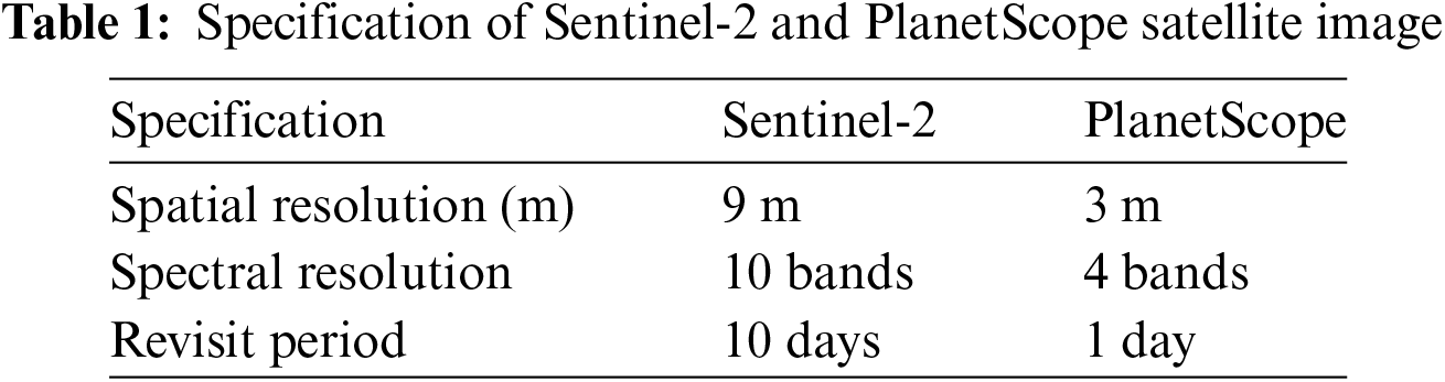
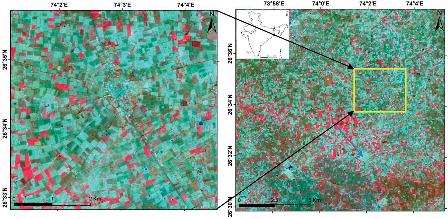
Figure 1: The actual study area is shown with a bounding box on the image

4  Adopted Methodology

The temporal indices database was initially built using pre-processed temporal multispectral images from Sentinel-2 satellite images. A database of temporal indices has been built using the CBSI-MSAVI-2 and MSAVI-2 indices approach. The main objective of the temporal indices database was to incorporate the phonological characteristics of the cumin and fennel plant and lower the spectral dimension by maintaining the temporal dimension and encoding items as vectors to be used in NC and PCM classifiers. The training sample operated as the “mean” and “individual sample as mean” in the supervised Noise Clustering (NC) and Possibilistic c-Means (PCM) algorithms. Fig. 2 illustrates the approach.

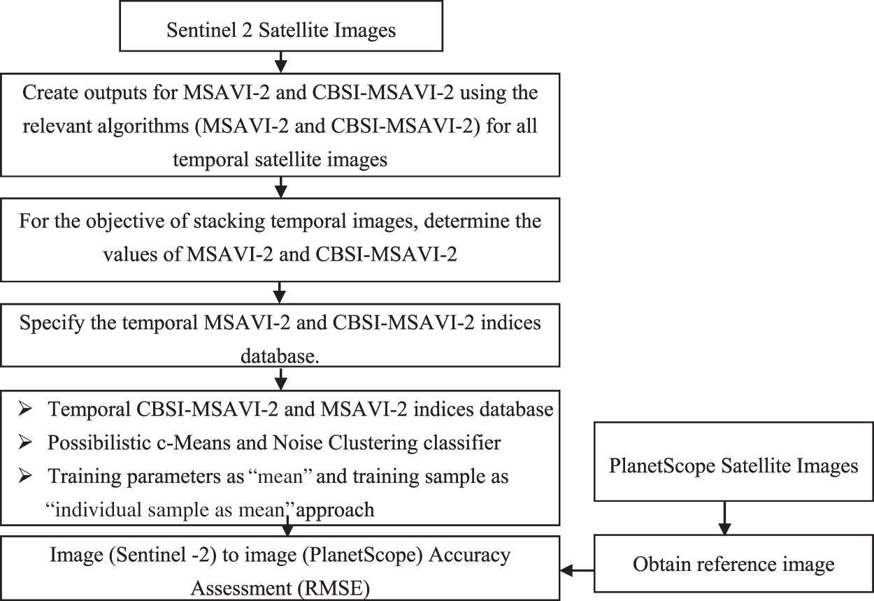
Figure 2: Methodology adopted

The temporal dataset was employed to map cumin and fennel crop fields using two training approaches. Images from the following dates generate the temporal dataset: 3 November 2021, 23 November 2021, 28 November 2021, 8 December 2021, 18 December 2021, 12 January 2022, 27 January 2022, 1 February 2022, 6 February 2022, 8 February 2022, 16 February 2022, and 21 February, 26 February, 13 March, 18 March, and 23 March 2022:

   i)  The MSAVI-2 and CBSI-MSAVI-2 indices for the cumin and fennel crop were calculated for temporal images using the MSAVI-2 and CBSI-MSAVI-2 formulas provided in Eqs. (8) and (9), respectively.

  ii)  Determine the CBSI-MSAVI-2 and MSAVI-2 values to find temporal images that are optimal and represent distinct stages of the cumin and fennel crop.

iii)  The dates of 13 March, 2018, and 23 are not suitable to consider for producing an optimal temporal indices database, according to the CBSI-MSAVI-2 and MSAVI-2 values computed in Step (2) (shown in Table 2, Figs. 3, and 4). However, the remaining temporal images are used to accomplish so.

 iv)  Training samples were selected from the CBSI-MSAVI-2 and MSAVI-2 databases after accounting for ground truth information gathered from sample sites around the study area. In this work 80 training samples for each crop are selected and applied these training samples to the entire given dataset.

  v)  The CBSI-MSAVI-2 and MSAVI-2 temporal datasets were categorized using the training sample as the “mean” and the “individual sample as the mean” in the NC and PCM classifier.

 vi)  To get the best result and algorithm, compare all of the outcomes after computing the Accuracy Assessment (RMSE) between Sentinel-2 and PlanetScope temporal images.

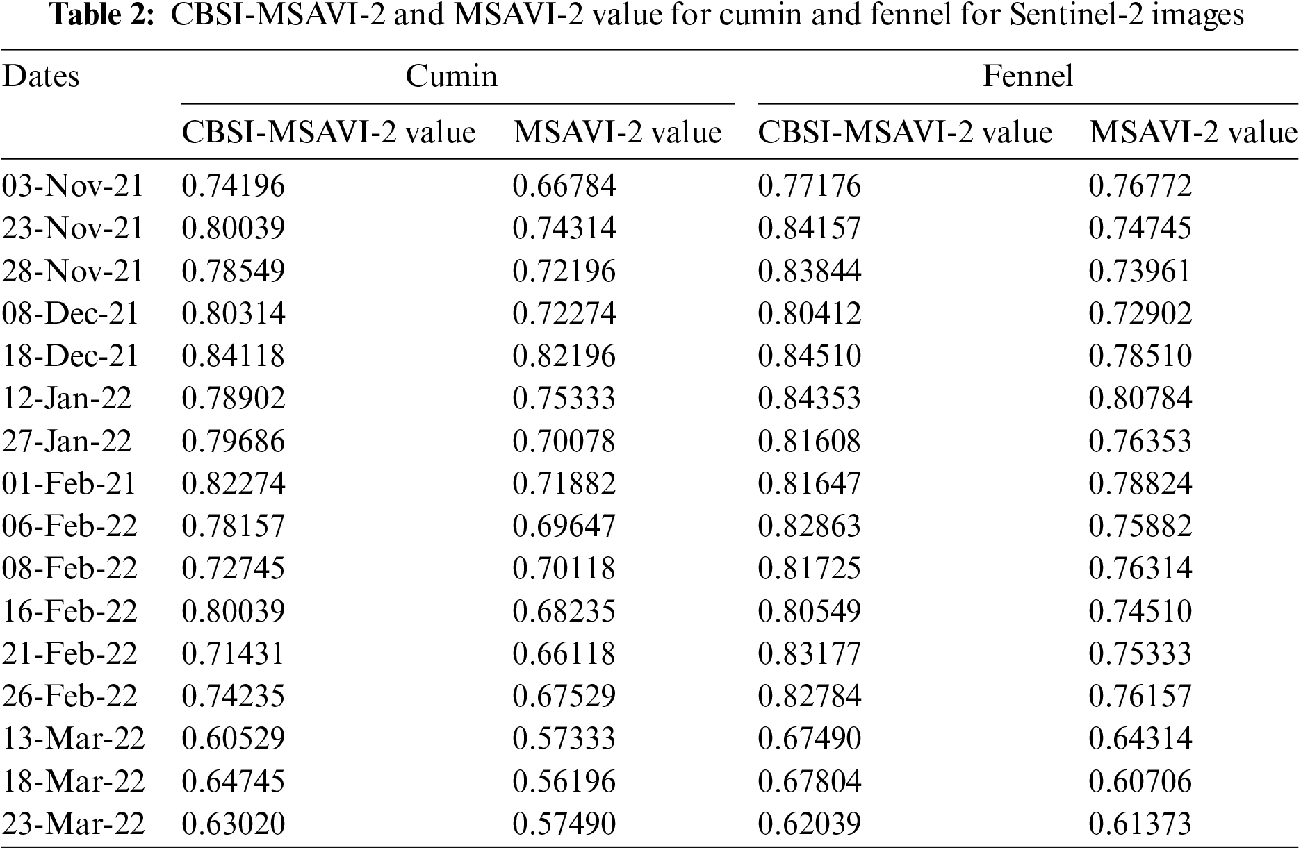
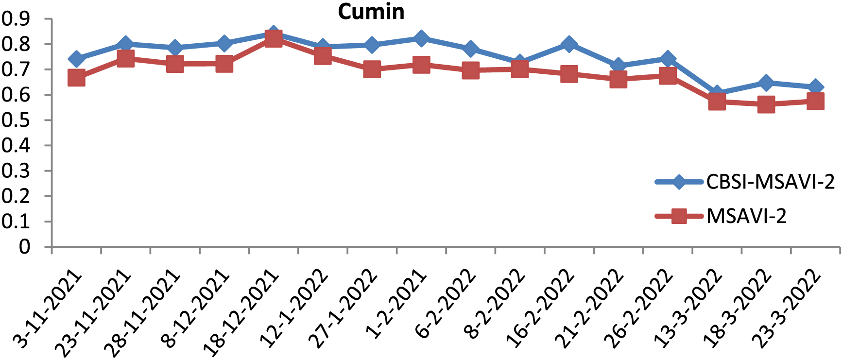
Figure 3: Graphical representation of CBSI-MSAVI-2 and MSAVI-2 values of Sentinel-2 image for cumin spices

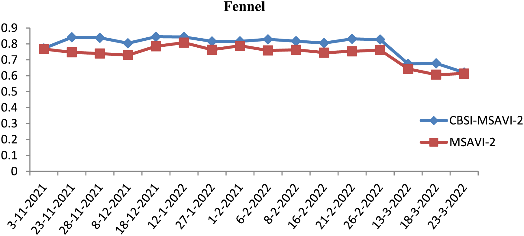
Figure 4: Graphical representation of CBSI-MSAVI-2 and MSAVI-2 values of Sentinel-2 image for fennel spices

The MSAVI-2 and CBSI-MSAVI-2 values for the cumin and fennel class from the temporal images for various dates are displayed in Table 2.

5  Results and Discussion

5.1 Optimizing Fuzziness Factor (m)

This section demonstrates the impact of the fuzziness factor (m), whose value varies from 1.1 to 3 with an interval of 0.2, on the CBSI-MSAVI-2 and MSAVI-2 temporal indices databases that were classified using PCM and NC classifiers employing training samples as “mean” and “individual samples as mean”. For each value of m, a Mean Membership Difference (MMD) analysis was used to determine the ideal value of m. The MMD displayed proximity results by comparing the membership value of the same training fields to the same test fields of the dataset, while the MMD displayed departure results by comparing the membership value of the different training fields to the different test fields. This paper calculated MMD proximity and departure results for cumin and fennel plants.

Table 3 displays the MMD proximity outcomes for the various values of m for the NC and PCM classifiers using the training sample as “mean” and “individual sample as mean” on the CBSI-MSAVI-2 and MSAVI-2 temporal indices database for the cumin plant. Cumin plant membership was used as the test field and the training field for the computation of MMD proximity.

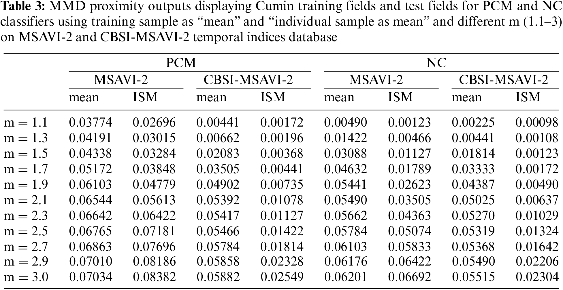
Table 4 displays the MMD proximity outcomes for the various values of m for the NC and PCM classifiers using the training sample as “mean” and “individual sample as mean” on the CBSI-MSAVI-2 and MSAVI-2 temporal indices database for the fennel plant. Fennel plant membership was used as the test field and the training field for the computation of MMD proximity.

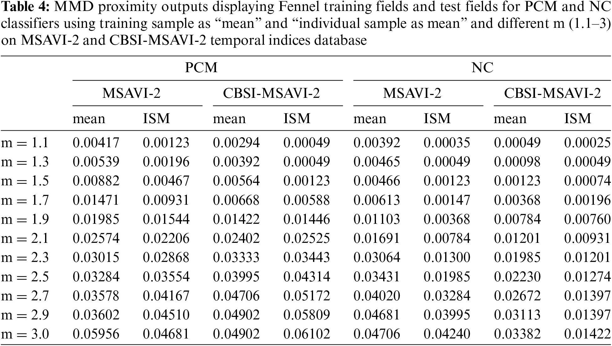
Table 5 displays the MMD Departure outcomes for the various values of m for the NC and PCM classifiers using the training sample as “mean” and “individual sample as mean” on the CBSI-MSAVI-2 and MSAVI-2 temporal indices database for the cumin plant. Here cumin plant membership is applied as a training field, and fennel plant membership is used as a testing field.

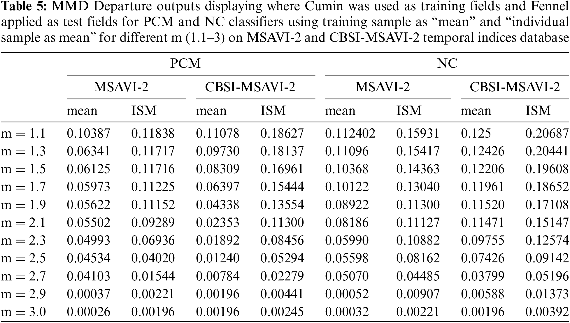
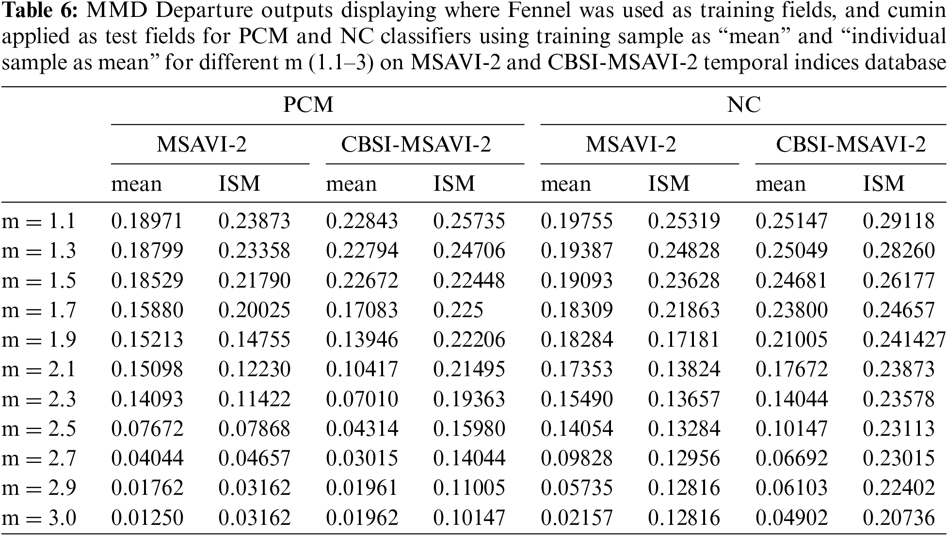
Table 6 displays the MMD Departure outcomes for the various values of m for the NC and PCM classifiers using the training sample as “mean” and “individual sample as mean” on the CBSI-MSAVI-2 and MSAVI-2 temporal indices database for the Fennel plant. Here fennel plant membership is applied as a training field, and cumin plant membership is used as a testing field.

5.2 Accuracy Assessment Using RMSE

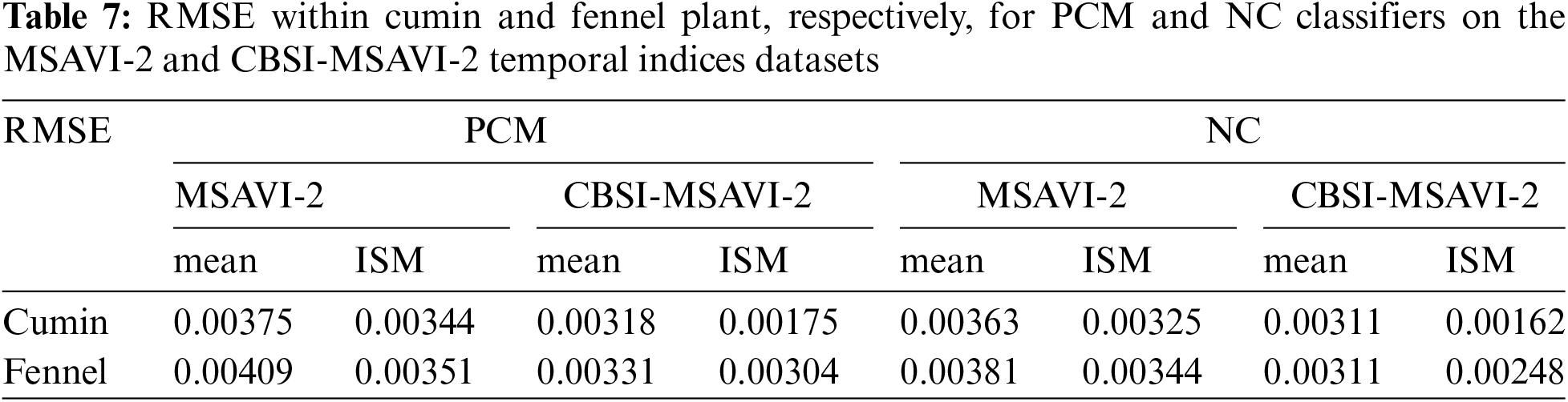
The accuracy of PCM and NC classifiers using training samples as “mean” and “individual sample as mean” is tested in this section by calculating the RMSE result. The result has been quantitatively analyzed using the RMSE method. The difference in membership values between the reference and classified data sets squared produces the RMSE [10]. Sentinel-2 was classified data set and reference data set from PlanetScope. A lower RMSE value denotes a successful classification [11]. The output of the PCM and NC classifiers using the training sample as “mean” and “individual sample as mean” along with different m (1.1–3) on the MSAVI-2 and CBSI-MSAVI-2 temporal indices is shown in Table 7.

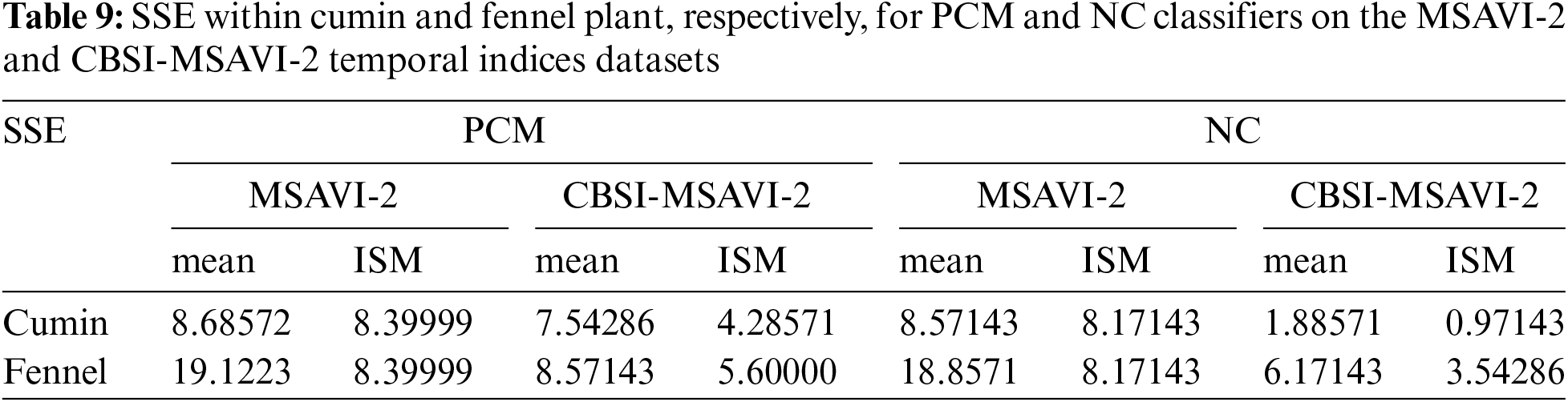
5.3 Cluster Validity and Variance

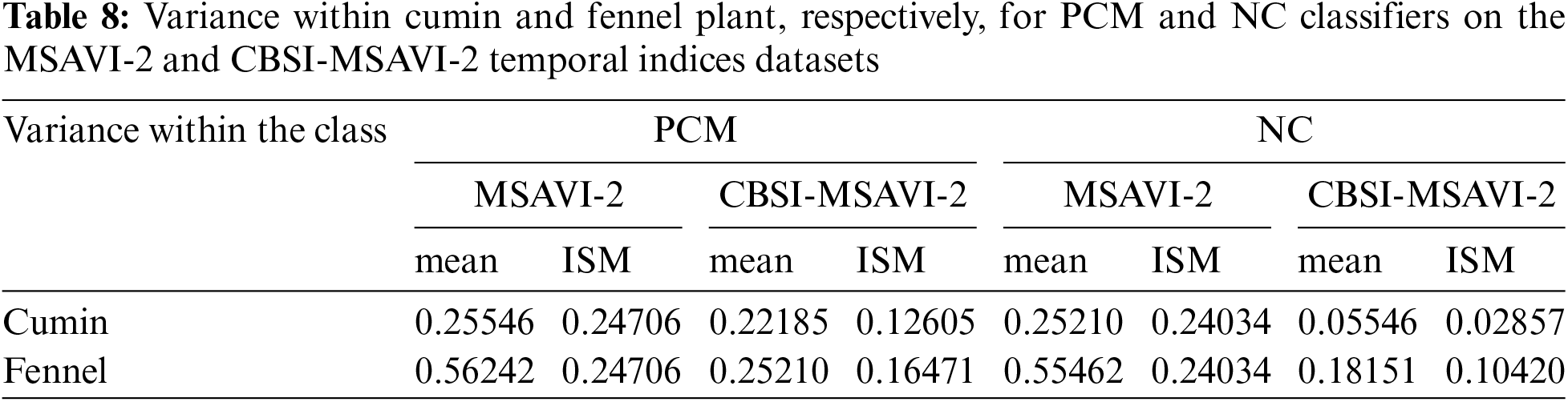
This section presents cluster validity and variance within the cumin and fennel plants. The sum of square errors (SSE) was utilized in this study project to analyze cluster validity in order to determine which clustering approach and temporal indices database produce the best results. Variance also reveals which approach successfully managed the heterogeneity within the fields. The minimum SSE and variance values get the best results. The variance within the cumin and fennel plant class for PCM and NC classifiers using training sample as “mean” and “individual sample as mean” on CBSI-MSAVI-2 and MSAVI-2 temporal indices datasets is displayed in Table 8.

The SSE within the cumin and fennel plant class for PCM and NC classifiers using training sample as “mean” and “individual sample as mean” on CBSI-MSAVI-2 and MSAVI-2 temporal indices datasets have been mentioned in Table 9.

5.4 Classified Outputs

The outputs of the cumin and fennel plant mapping class have been shown in this section. These classified outputs used NC and PCM classifiers applying training samples as “mean” and “individual sample as mean” to categorize the CBSI-MSAVI-2 and MSAVI-2 temporal indices database. The results of applying the training sample as “mean” and “individual sample as mean” to the CBSI-MSAVI-2 and MSAVI-2 temporal indices databases using NC and PCM classifiers have been shown in Figs. 5–8. The results in Figs. 5–8 demonstrate that when the training sample was configured as “individual sample as mean,” the CBSI-MSAVI-2 temporal indices database produced better-classified fields. The red circle indicates that Cumin and Fennel fields, found during ground truth work, have been appropriately classified.

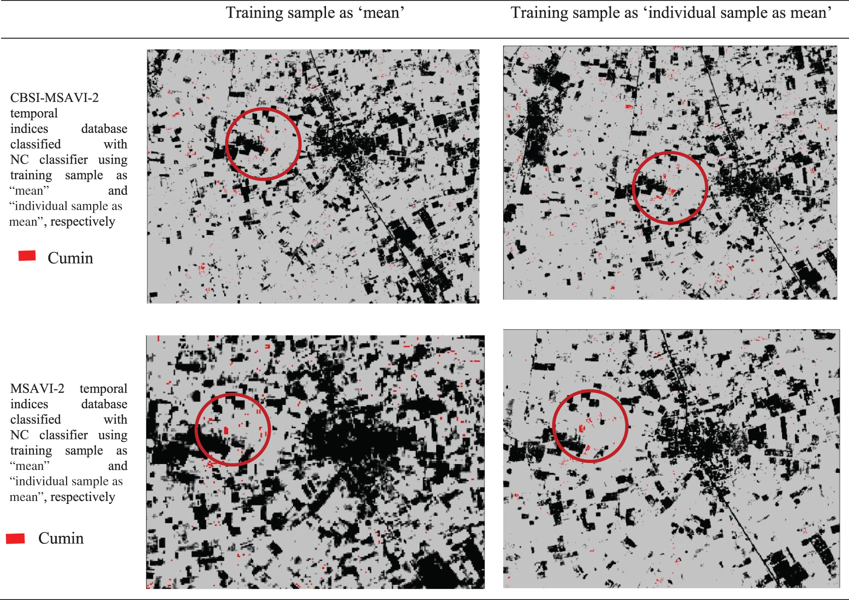
Figure 5: Comparison of training sample approach as “mean” and “individual sample as mean” outputs for NC classifiers. The red circle denotes appropriately classified Cumin fields that were discovered during ground truth work

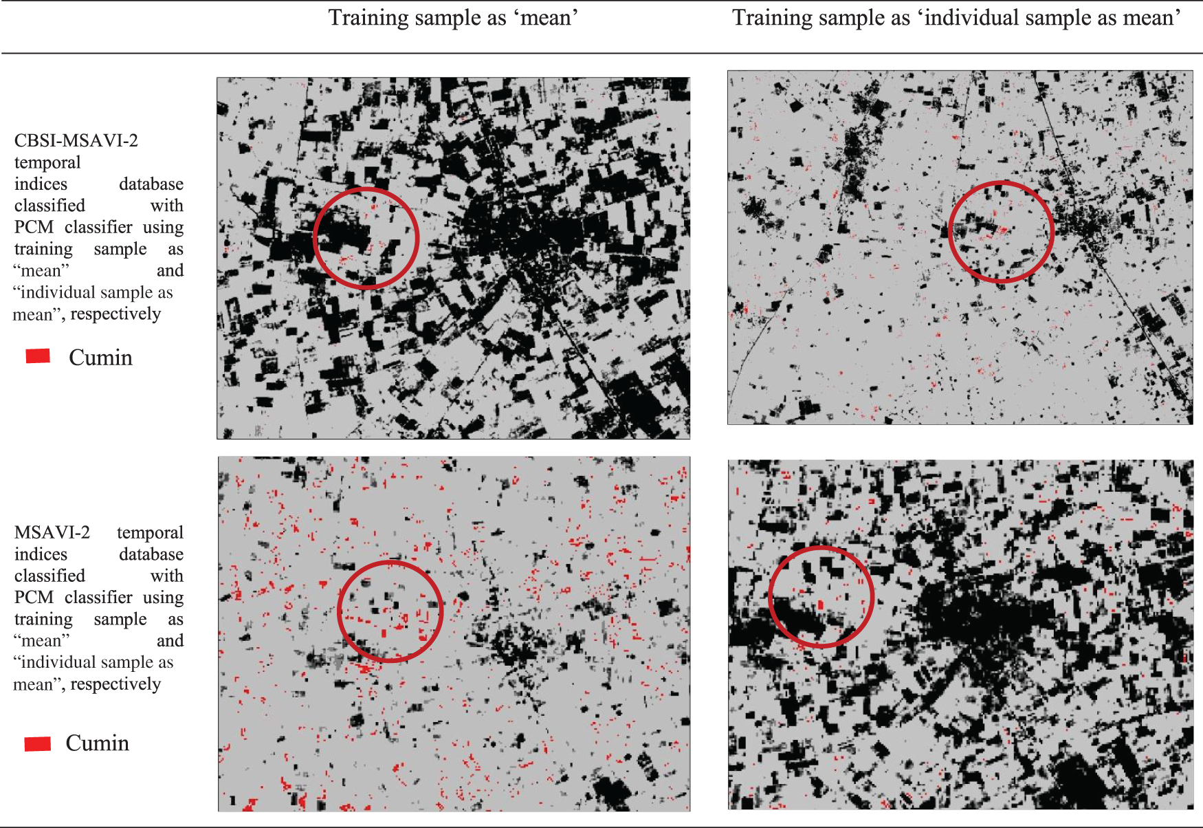
Figure 6: Comparison of training sample approach as “mean” and “individual sample as mean” outputs for PCM classifiers. The red circle denotes appropriately classified cumin fields that were discovered during ground truth work

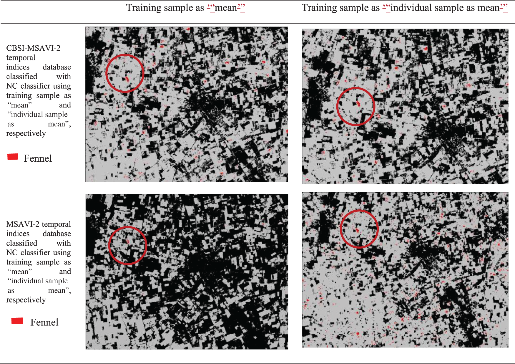
Figure 7: Comparison of training sample approach as ‘mean’ and ‘individual sample as mean’ outputs for NC classifiers. The red circle denotes appropriately classified Fennel fields that were discovered during ground truth work

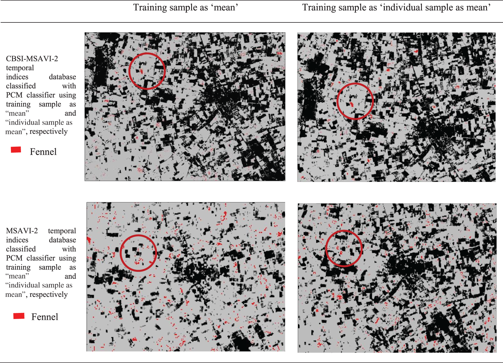
Figure 8: Comparison of training sample approach as “mean” and “individual sample as mean” outputs for PCM classifiers. The red circle denotes appropriately classified Fennel fields that were discovered during ground truth work

6  Discussions

The impact of the fuzziness factor (m) on the classification accuracy of temporal indices databases, specifically CBSI-MSAVI-2 and MSAVI-2, using PCM and NC classifiers with training samples configured as either “mean” or “individual samples as mean.” The Mean Membership Difference (MMD) analysis determined optimal m values by comparing membership values between training and test fields, focusing on cumin and fennel plants. Results indicated that lower m values generally yielded better proximity results, while higher m values improved departure outcomes. The accuracy assessment using RMSE revealed that the “individual sample as mean” approach consistently produced lower RMSE values, signifying superior classification performance. Furthermore, cluster validity and variance analyses, quantified by SSE and variance within classes, demonstrated that the “individual sample as mean” approach effectively managed field heterogeneity, resulting in lower SSE and variance values. Classified outputs, visualized in Figs. 5–8, confirmed that the CBSI-MSAVI-2 database provided better classification, particularly when employing the “individual sample as mean” approach, accurately identifying cumin and fennel fields during ground truth verification.

This study shows the research on the impact of the fuzziness factor (m) in fuzzy classification systems. Similar to studies by [35,36], our results show that lower m values yield better proximity results, while higher m values enhance departure outcomes. This observation is consistent with the fundamental principles of fuzzy set theory, where the fuzziness parameter modulates the degree of membership overlap among classes.

However, our study uniquely highlights the “individual sample as mean” approach’s superiority in classification accuracy, as evidenced by lower RMSE values. This finding contrasts with the more traditional “mean” approach discussed in [22,23], where the mean of the training samples was found to suffice in certain scenarios. Our results suggest that considering the individuality of each sample captures the field heterogeneity more effectively, a critical factor when dealing with agricultural datasets where plant phenology can vary significantly.

Furthermore, the CBSI-MSAVI2MSAVI-2 database outperformed the MSAVI2MSAVI-2 in classification tasks. This advantage is attributable to the combined benefits of CBSI and MSAVI-2 indices, which provide a more nuanced representation of vegetation characteristics. The integration of these indices likely contributes to the enhanced classification accuracy, as also noted by [31] in their comparative studies of spectral indices for vegetation monitoring.

Despite these promising results, our research is subject to several limitations. Firstly, the study was confined to a specific geographical region and focused on cumin and fennel plants. The generalizability of our findings to other crops and regions remains to be validated. Additionally, the temporal scope of our dataset was limited, which may not capture the full spectrum of phenological variations. Future studies should consider longer time series data to better understand the seasonal dynamics of crop growth.

Secondly, the selection of the fuzziness factor (m) was based on Mean Membership Difference (MMD) analysis. While this method is robust, it may not be universally optimal for all datasets. Alternative methods for determining the optimal m value, such as cross-validation or entropy-based approaches, could provide additional insights and potentially improve classification accuracy.

Future research should aim to expand the spatial and temporal scope of the study. Incorporating a diverse range of crops and extending the analysis across different climatic zones would enhance the robustness and applicability of the findings. Moreover, integrating additional spectral indices and advanced remote sensing techniques, such as hyperspectral imaging and LiDAR, could further improve classification accuracy and field heterogeneity management.

7  Conclusions

This study determines which fuzzy-based approach better mapped cumin and fennel fields, using PCM and NC classifiers with the “mean” and “individual training sample as mean” training selection procedures. These outcomes were considered utilizing the CBSI-MSAVI-2 and MSAVI-2 temporal indices database. Using Sentinel-2 satellite images taken between 3 November, 2021, and 23 March, 2022, the temporal indices database was created. To determine whether algorithms perform better, the following metrics were calculated: RMSE, MMD, Variance, and SSE (cluster analysis). The best outcome was obtained when the NC classifier used the CBSI-MSAVI-2 temporal indices with “individual sample as mean.” NC classifier using “individual sample as mean” for m = 1.1, the RMSE, MMD, Variance, and SSE values for the NC classifier using “individual sample as mean” on the CBSI-MSAVI-2 temporal indices for cumin were 0.00098, 0.00162, 0.02857, and 0.97143, respectively and for fennel were 0.00025, 0.00248, 0.10420, and 3.54286, respectively. The PCM classifier with the “individual sample as mean” approach provides an excellent result compared to the “mean” training sample using the CBSI-MSAVI-2 temporal indices database. For the m = 1.1, the RMSE, MMD, Variance, and SSE values for the PCM classifier on the CBSI-MSAVI-2 temporal indices using “individual sample as mean” were 0.02745, 0.01961, 0.17885, and 6.97515, respectively. The outcome showed that the NC classifier using the CBSI-MSAVI-2 temporal indices with “individual sample as mean” provides the best-classified result while appropriately mapping and managing heterogeneity within the class.

Acknowledgement: None.

Funding Statement: The authors received no specific funding for this study.

Author Contributions: The authors confirm contribution to the paper as follows: study conception and design: Shilpa Suman, Anil Kumar; data collection: S. K. Tiwari; analysis and interpretation of results: Shilpa Suman, Abhishek Rawat; draft manuscript preparation: Abhishek Rawat, Shilpa Suman. All authors reviewed the results and approved the final version of the manuscript.

Availability of Data and Materials: The satellite data used in the study is available in respective website portal, and can be downloaded.

Ethics Approval: Not applicable.

Conflicts of Interest: The authors declare that they have no conflicts of interest to report regarding the present study.

References

1. Mohamed S, Shehata AG, Essam M, Ali H, Olwy EA, Abdulrshed A, et al. Elucidating the antioxidant potency and polyphenolic profiles of medicinal herbs through voltammetric and colorimetric techniques. Sohag J Sci. 2024;9(4):415–22. doi:10.21608/sjsci.2024.285588.1198. [Google Scholar] [CrossRef]

2. Pirzad A, Darvishzadeh R, Hassani A. Effect of superabsorbent application under different irrigation regimes on photosynthetic pigments in cuminum cyminum and its relation with seed and essential oil yield. J Hortic Sci. Sep 2015;29(3):377–87. doi:10.22067/jhorts4.v0i0.27389. [Google Scholar] [CrossRef]

3. Meena MD, Vishal MK, Khan MA. Market arrivals and prices behavior of cumin in India. Int J Curr Microbiol Appl Sci. 2021;10(1):528–36. doi:10.20546/ijcmas.2021.1001.064. [Google Scholar] [CrossRef]

4. Barros L, Carvalho AM, Ferreira ICFR. The nutritional composition of fennel (Foeniculum vulgare): shoots, leaves, stems and inflorescences. LWT-Food Sci Technol. 2010;43(5):814–8. doi:10.1016/j.lwt.2010.01.010. [Google Scholar] [CrossRef]

5. Malhotra SK. Fennel and fennel seed. In: Handbook of herbs and spices. Woodhead Publishing: Elsevier; Jan. 1, 2012. p. 275–302. doi:10.1533/9780857095688.275. [Google Scholar] [CrossRef]

6. Shamsuzzoha M, Noguchi R, Ahamed T. Rice yield loss area assessment from satellite-derived NDVI after extreme climatic events using a fuzzy approach. Agric Inf Res. 2022;31(1):32–46. doi:10.3173/air.31.32. [Google Scholar] [CrossRef]

7. Tayyebi A, Delavar MR, Saeedi S, Amini J, Alini H. Monitoring land use change by multi-temporal landsat remote sensing imagery. Int Arch Photogramm Remote Sens Spat Inf Sci. 2008;37(B7):1037–42. doi:10.13140/2.1.2736.3204. [Google Scholar] [CrossRef]

8. Faruque MJ, Vekerdy Z, Hasan MY, Ziaul Islam K, Young B, Tofayal Ahmed M, et al. Monitoring of land use and land cover changes by using remote sensing and GIS techniques at human-induced mangrove forests areas in Bangladesh. Remote Sens Appl Soc Environ. 2022;25:100699. doi:10.1016/j.rsase.2022.100699. [Google Scholar] [CrossRef]

9. Güler M, Yomralıoğlu T, Reis S. Using landsat data to determine land use/land cover changes in Samsun, Turkey. Environ Monit Assess. 2007;127(1):155–67. doi:10.1007/s10661-006-9270-1. [Google Scholar] [PubMed] [CrossRef]

10. Fichera CR, Modica G, Pollino M. Land cover classification and change-detection analysis using multi-temporal remote sensed imagery and landscape metrics. Eur J Remote Sens. 2012;45(1):1–18. doi:10.5721/EuJRS20124501. [Google Scholar] [CrossRef]

11. Musande V, Kumar A, Roy PS, Kale K. Evaluation of fuzzy-based classifiers for cotton crop identification. Geocarto Int. 2013;28(3):243–57. doi:10.1080/10106049.2012.685894. [Google Scholar] [CrossRef]

12. Loureiro AAF, Nogueira JMS, Cunha FD, Macedo DF, Mota VFS. Protocols, mobility models and tools in opportunistic networks: a survey. Comput Commun. 2014;48:5–19. doi:10.1016/j.comcom.2014.03.019. [Google Scholar] [CrossRef]

13. Ferchichi A, Ben Abbes A, Barra V, Farah IR. Forecasting vegetation indices from spatio-temporal remotely sensed data using deep learning-based approaches: a systematic literature review. Ecol Inform. 2022;68:101552. doi:10.1016/j.ecoinf.2022.101552. [Google Scholar] [CrossRef]

14. Lv TT, Liu C. Study on extraction of crop information using time-series MODIS data in the Chao Phraya Basin of Thailand. Adv Sp Res. 2010;45(6):775–84. doi:10.1016/j.asr.2009.11.013. [Google Scholar] [CrossRef]

15. Dutta A, Kumar A, Sarkar S. Suitable sampling technique in contextual fuzzy c-means classification of remotely sensed data for land cover mapping. Geocarto Int. 2010;25(5):369–78. doi:10.1080/10106041003731300. [Google Scholar] [CrossRef]

16. Verbesselt J, Hyndman R, Newnham G, Culvenor D. Detecting trend and seasonal changes in satellite image time series. Remote Sens Environ. 2010;114(1):106–15. doi:10.1016/j.rse.2009.08.014. [Google Scholar] [CrossRef]

17. Keshava N, Mustard JF. Spectral unmixing. IEEE Signal Process Mag. 2002;19(1):44–57. doi:10.1109/79.974727. [Google Scholar] [CrossRef]

18. Zhang J, Foody GM. Fully-fuzzy supervised classification of sub-urban land cover from remotely sensed imagery: statistical and artificial neural network approaches. Int J Remote Sens. 2001;22(4):615–28. doi:10.1080/01431160050505883. [Google Scholar] [CrossRef]

19. Bezdek JC, Ehrlich R, Full W. FCM: the fuzzy c-means clustering algorithm. Comput Geosci. 1984;10(2–3):191–203. doi:10.1016/0098-3004(84)90020-7. [Google Scholar] [CrossRef]

20. Krishnapuram R, Keller JM. A possibilistic approach to clustering. IEEE Trans Fuzzy Syst. 1993;1(2):98–110. doi:10.1109/91.227387. [Google Scholar] [CrossRef]

21. Dave RN, Sen S. Noise clustering algorithm revisited. In: 1997 Annu Conf North Am Fuzzy Inf Process Soc-NAFIPS (Cat. No. 97TH8297), Sep. 21, 1997; Syracuse, NY, USA. p. 199–204. doi:10.1109/NAFIPS.1997.624037. [Google Scholar] [CrossRef]

22. Suman S, Kumar A, Kumar D, Soni A. Augmenting possibilistic c-means classifier to handle noise and within class heterogeneity in classification. J Appl Remote Sens. 2021;15(4):1–17. doi:10.1117/1.JRS.15.044509. [Google Scholar] [CrossRef]

23. Jose N, Kumar A. Handling heterogeneity through ‘individual sample as mean’ approach–A case study of Isabgol (Psyllium husk) medicinal crop. Remote Sens Appl Soc Environ. Jan. 1, 2022;25:100671. doi:10.1016/j.rsase.2021.100671. [Google Scholar] [CrossRef]

24. Sivaraj P, Kumar A, Koti SR, Naik P. Effects of training parameter concept and sample size in possibilistic c-Means classifier for pigeon pea specific crop mapping. Geomatics. 2022;2(1):107–24. doi:10.3390/geomatics2010007. [Google Scholar] [CrossRef]

25. Narayanan J, Kothari M, Pathak S, Jeyseelan AT. Assessing drought for arid regions using satellite derived vegetation index (MSAVI2) and TRMM data. Indian Cartogr. 2013;32:421–7. [Google Scholar]

26. Krishnapuram R, Keller JM. The possibilistic C-means algorithm: insights and recommendations. IEEE Trans Fuzzy Syst. Aug. 1996;4(3):385–93. doi:10.1109/91.531779. [Google Scholar] [CrossRef]

27. Yan L, Roy DP. Improved time series land cover classification by missing-observation-adaptive nonlinear dimensionality reduction. Remote Sens Environ. 2015;158:478–91. doi:10.1016/j.rse.2014.11.024. [Google Scholar] [CrossRef]

28. Ni R, Zhu X, Lei Y, Li X, Dong W, Zhang C, et al. Effectiveness of common preprocessing methods of time series for monitoring crop distribution in Kenya. Agriculture. Jan. 7, 2022;12(1):79. doi:10.3390/agriculture12010079. [Google Scholar] [CrossRef]

29. Gelman A. Data analysis using regression and multilevel/hierarchical models. Cambridge University Press; 2007. [Google Scholar]

30. Mustikaningrum D, Widya LK, Ulfah U, Wijayanti RF. Flood susceptibility mapping using machine learning in Kening River, Sub Watershed of Bengawan Solo, Tuban. Indones J Urban Environ Technol. Jul. 20, 2024;183–200. doi:10.25105/urbanenvirotech.v7i2.18818. [Google Scholar] [CrossRef]

31. Suman S, Kumar A, Rawat A. Fuzzy machine learning based algorithms for mapping chickpea agricultural crop fields using sentinel-2 satellite data. J Geomatics. 2024;18(1):40–9. doi:10.58825/jog.2024.18.1.101. [Google Scholar] [CrossRef]

32. Qi J, Chehbouni A, Huete AR, Kerr YH, Sorooshian S. A modified soil adjusted vegetation index. Remote Sens Environ. 1994;48(2):119–26. doi:10.1016/0034-4257(94)90134-1. [Google Scholar] [CrossRef]

33. Dehghan H, Ghassemian H. Measurement of uncertainty by the entropy: application to the classification of MSS data. Int J Remote Sens. 2006;27(18):4005–14. [Google Scholar]

34. Bostanci B, Bostanci E. An evaluation of classification algorithms using Mc Nemar’s test. Adv Intell Syst Comput. 2013;201:15–26. [Google Scholar]

35. Kumar A, Upadhyay P, Kumar AS. Fuzzy machine learning algorithms for remote sensing image classification. Boca Raton:CRC Press; Jul. 19, 2020. doi:10.1080/01431160600647225. [Google Scholar] [CrossRef]

36. Suman S, Kumar D, Kumar A. Study the effect of convolutional local information-based Fuzzy c-Means classifiers with different distance measures. J Indian Soc Remote Sens. 2021;49(7):1561–8. doi:10.1007/s12524-021-01333-6. [Google Scholar] [CrossRef]