
 Submit a Paper
 Propose a Special lssue
 Open Access
ARTICLE
Digital Soil Mapping (DSM) Using a GIS-Based RF Machine Learning Model: The Case of Strandzha Mountains (Thrace Peninsula, Türkiye)
1 Department of Geography, Faculty of Arts and Sciences, Tekirdag Namık Kemal University, Tekirdag, 59030, Türkiye
2 Department of Soil Sciences and Plant Nutrition, Faculty of Agriculture, Tekirdag Namık Kemal University, Tekirdag, 59030, Türkiye
* Corresponding Author: Emre Ozsahin. Email:
Revue Internationale de Géomatique 2024, 33, 341-361. https://doi.org/10.32604/rig.2024.054197
Received 21 May 2024; Accepted 14 August 2024; Issue published 13 September 2024
 View Full Text
 Download PDF
Abstract
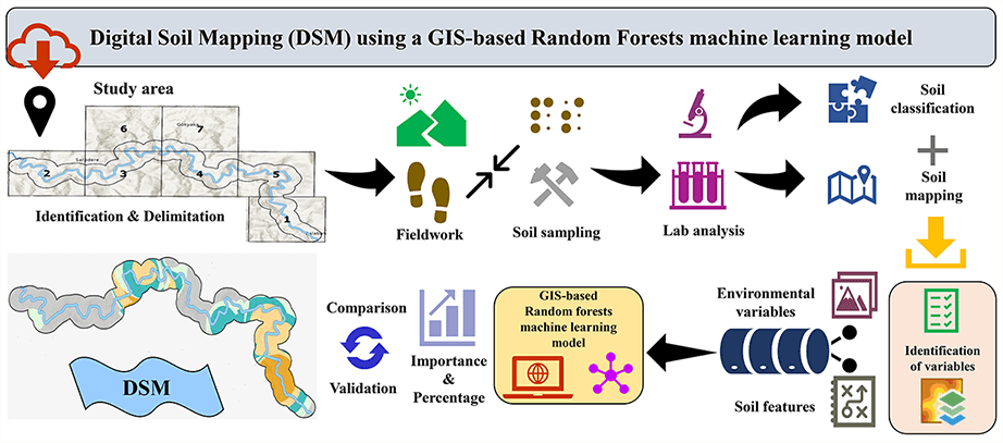
This study assessed and mapped the spatial distribution of soil types and properties developed under the forest cover of the Strandzha Mountains of Türkiye. The study was conducted on a micro-scale in the riparian zone of the Balaban River, which characterizes the soils distributed in the mountainous area. The effect of environmental factors on the spatial distribution of soil types and properties was also determined. To gather data, soil sampling, laboratory analysis, data processing and mapping were sequentially performed. These data were analyzed using the Geographical Information System (GIS) based Random Forest (RF) machine learning technique. Digital Soil Mapping (DSM) was developed with satisfactory performance. DSM suggests that the factors affecting the spatial distribution of soil types and properties in the sample area are, from most important to least important, topography (50.77%), climate (28.14%), organisms (8.22%), parent material (7.24%) and time (5.63%). With the contributions of all these factors in different proportions, it was determined that soils belonging to the Entisol and then Inceptisol orders were the most widespread in the sample area. The study results revealed that the GIS-based RF machine-learning technique can be used as a reliable tool for the development of DSM in mountainous terrains.Graphic Abstract
Keywords
Soil is an essential and primary component of life on earth [1]. It plays a significant role in human life and well-being [2,3]. Soil is the largest terrestrial organic carbon sink [4]. It is a multifunctional system with substantial contributions to ecosystem services such as food production, climate regulation, nutrient cycling, biochemical transformations, and pest control [5,6].
Soil is a heterogeneous system and exhibits spatially diverse properties [7]. These characteristics are key in ecological modeling, environmental forecasting, precision agricultural practices, and natural resource management [8]. Pedogenic processes may lead to the formation of different soil types [9]. Hence, the relationships between the spatial distribution of soil types, soil properties, and environmental factors should be well-comprehended [10] since such relationships are considered key indicators for soil management and sustainable land use [11]. Faster, quantitative, and objective tools and methods have been developed to analyze such relationships [12].
Recently, Geographic Information Systems (GIS) based methods have been used to understand better the complex relationship between soil and environment [13] and to reveal information on spatial variability of soil properties. Machine learning (ML) techniques are widely used [14–17]. These techniques provide more information about unsampled points by examining non-linear interactions to predict the effects of environmental variables on soil properties and their spatial variation [18]. Widely used ML techniques [19,20] include Random Forest (RF) [21,22], Quantile Regression Forest (QRF) [23], Cubist [24], Regression Tree (RT) [25], Neural Network (NN) [26], Support Vector Machines (SVM) [27] and Bayesian approaches [28].
The Strandzha Mountains are the most important landforms of the Balkan Peninsula, which corresponds to the southeastern part of the European continent. The mountains extend along the Black Sea coast on southeastern Bulgaria and northwestern Türkiye borders and have a privileged forest cover with unique flora [29]. Therefore, the main use of the land in these mountains is forestry [30]. Some soils in these mountains, which form a special ecosystem compared to their surroundings, are considered unique soils of the Balkan Peninsula [31]. It was reported in a previous study that the soils of the Strandzha Mountains differ spatially in their influence on forest vegetation as compared to soils in surrounding areas [32]. Various soil studies have been conducted in Bulgaria [33] and Türkiye [29,30,34–37] to determine these differences. Although the relationship between the spatial distribution of soil types and environmental factors has been emphasized especially in studies conducted in Türkiye, there is still an important gap in the literature since no study has analyzed this relationship in detail with Digital Soil Mapping (DSM) developed using a GIS-based RF.
This study was conducted to assess and map the spatial distribution of soil types and properties under forest cover in the Strandzha Mountains of Türkiye. The study was conducted on a micro-scale, focusing on the riparian zone of the Balaban River, which more typically characterizes the soils distributed in the mountainous area. Thus, another objective was to distinguish and examine features important for diagnosing soil processes, such as content, quantity, mobility, degree of transformation, and localization [38]. This study is unique in revealing soil types and properties in the forest ecosystem of the Strandzha Mountains with a biodiversity-rich landscape for the European continent, Balkan Peninsula, and Türkiye. So far, although numerous studies [39–41] have been conducted with GIS-based RF method for soil mapping in different parts of the world and various climates, the most important contribution of this study to the scientific literature is that it is the first attempt in the Strandzha Mountains in Türkiye’s Thrace. This study also reveals the ongoing pedogenic evolution of a region and the factors affecting this process of evolution.
The study area corresponds to the riparian zone of the Balaban River in the Strandzha Mountains of Türkiye (Fig. 1). This area, which lies between the river channel and the upland, was chosen because it is a very heterogeneous place in time and space [42] regarding microclimate, topography, and parent material, especially soil, compared to its surroundings. The study area has many ecosystem functions and services and complex biological, chemical, and physical interactions. Therefore, the study area, which functions as a critical transition zone, was delimited as a 500 m wide zone (Fig. 1), taking into account the size and location of the drainage system, hydrological and geomorphological characteristics [43], as reported in the literature [7,44].
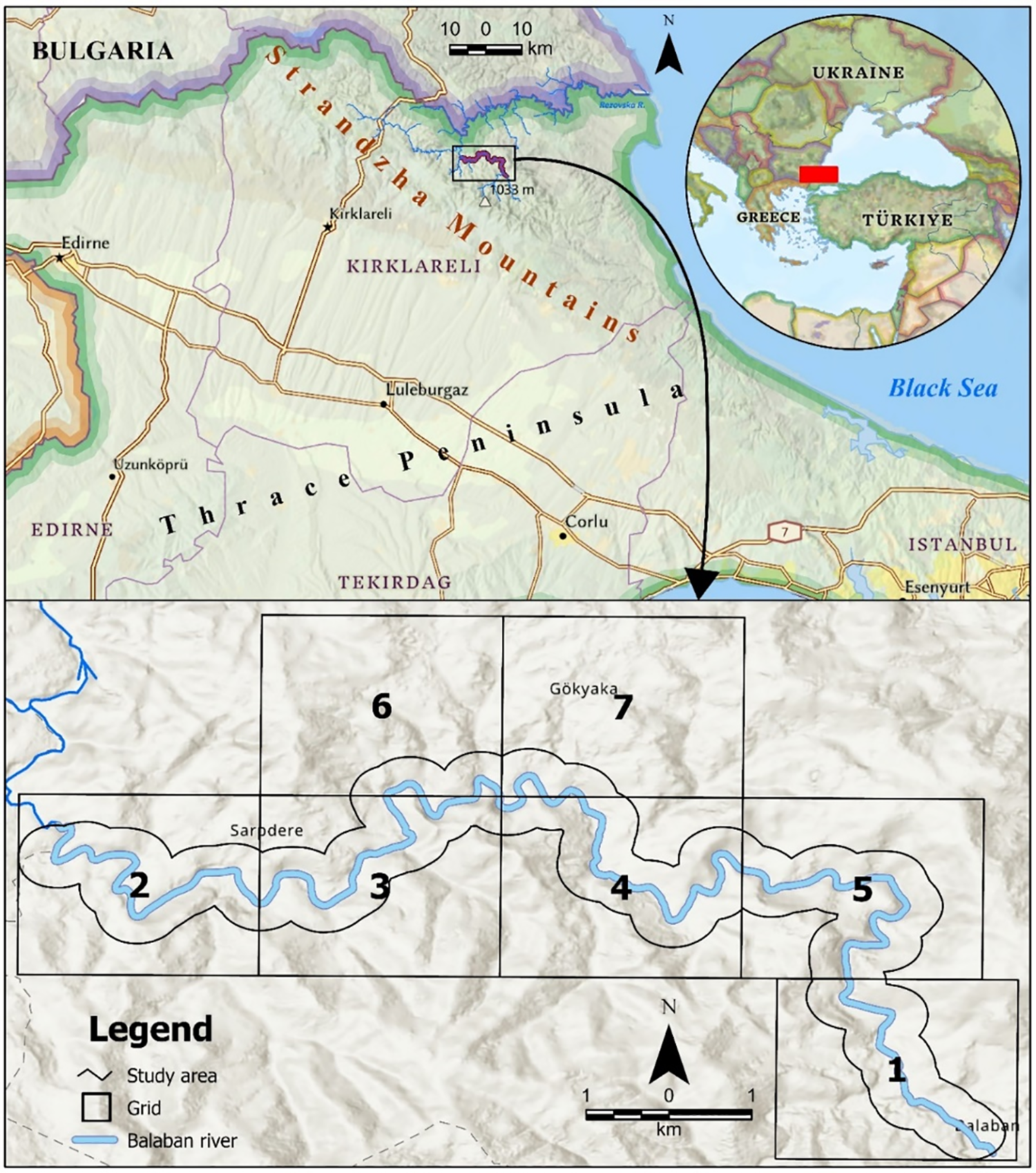
Figure 1: Location map of the study area
The study area is located on the Strandzha Massif and commonly consists of Paleozoic-aged metamorphic rocks such as gneiss, metagranitoid, schist, marble, and quartzite [45]. Quaternary alluvium is spread over the river valley floors. The study area has a topography shaped by the Balaban River and its tributaries, originating from the high parts of the Strandzha Mountains. The study area’s elevation varies between 300–555 m [46]. According to the Köppen-Geiger climate classification, “Fully humid temperate, warm summer (temperate oceanic) (Cfb)” climate is dominant in the study area [47]. Based on these climate characteristics, it was determined that the soil moisture regime of the study area and its immediate surroundings is xeric and the temperature regime is thermic [29]. Beech, hornbeam, and oak trees cover a large area within the forest cover of the study area [48], there are also grassland, cropland, bare/sparse vegetation, and built-up land cover [49,50].
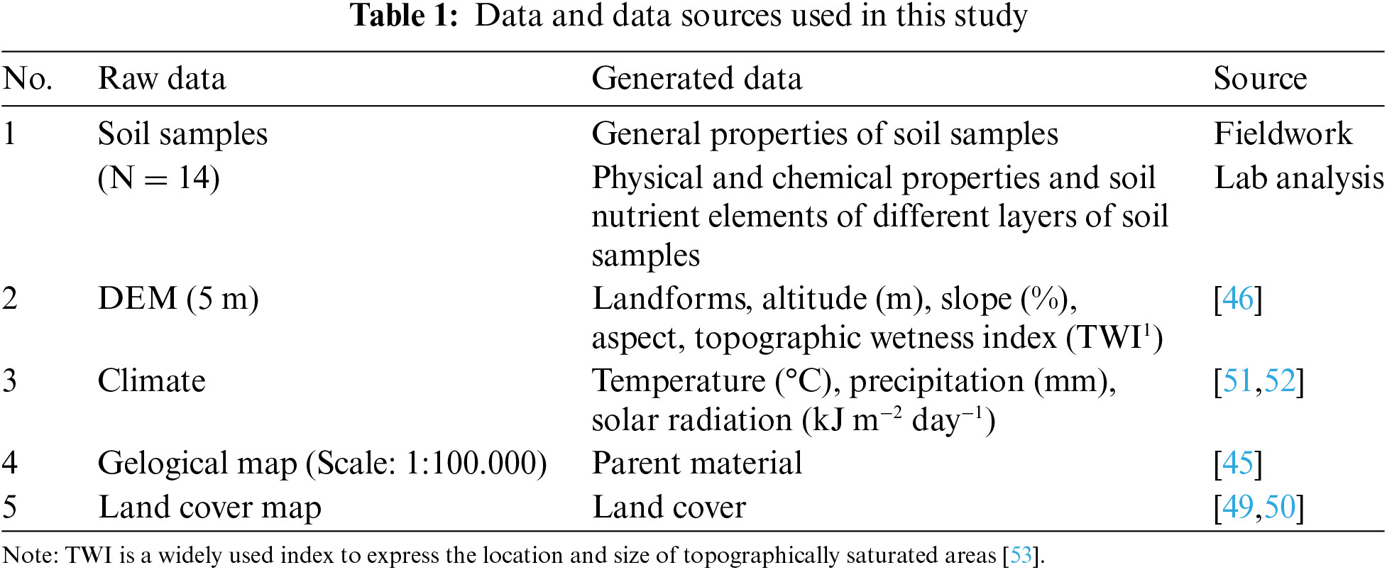
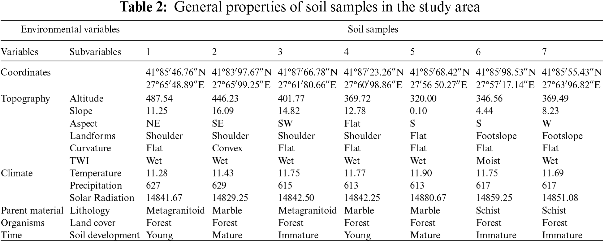
In this study, analysis results of soil samples taken according to the environmental conditions (topographic features, climate, land cover, etc.) affecting soil properties of the study area were used as the primary material. Topographic features were determined by GIS techniques based on Digital Elevation Model (DEM) data [46]. Data on climate characteristics were obtained from the WorldClim database [51,52]. The parent material and land cover data were obtained from geology [45] and land cover [49,50] maps, respectively (Table 1).
DSM was developed using a GIS-based RF. The study was scaled to a high resolution (Resolution: 5 m) due to the extent and possibilities offered by the boundaries of the study area and the data on other environmental factors. The study was carried out in three phases: field works (soil sampling), laboratory analysis of soil samples, and classification and mapping of soil types (Fig. 2).
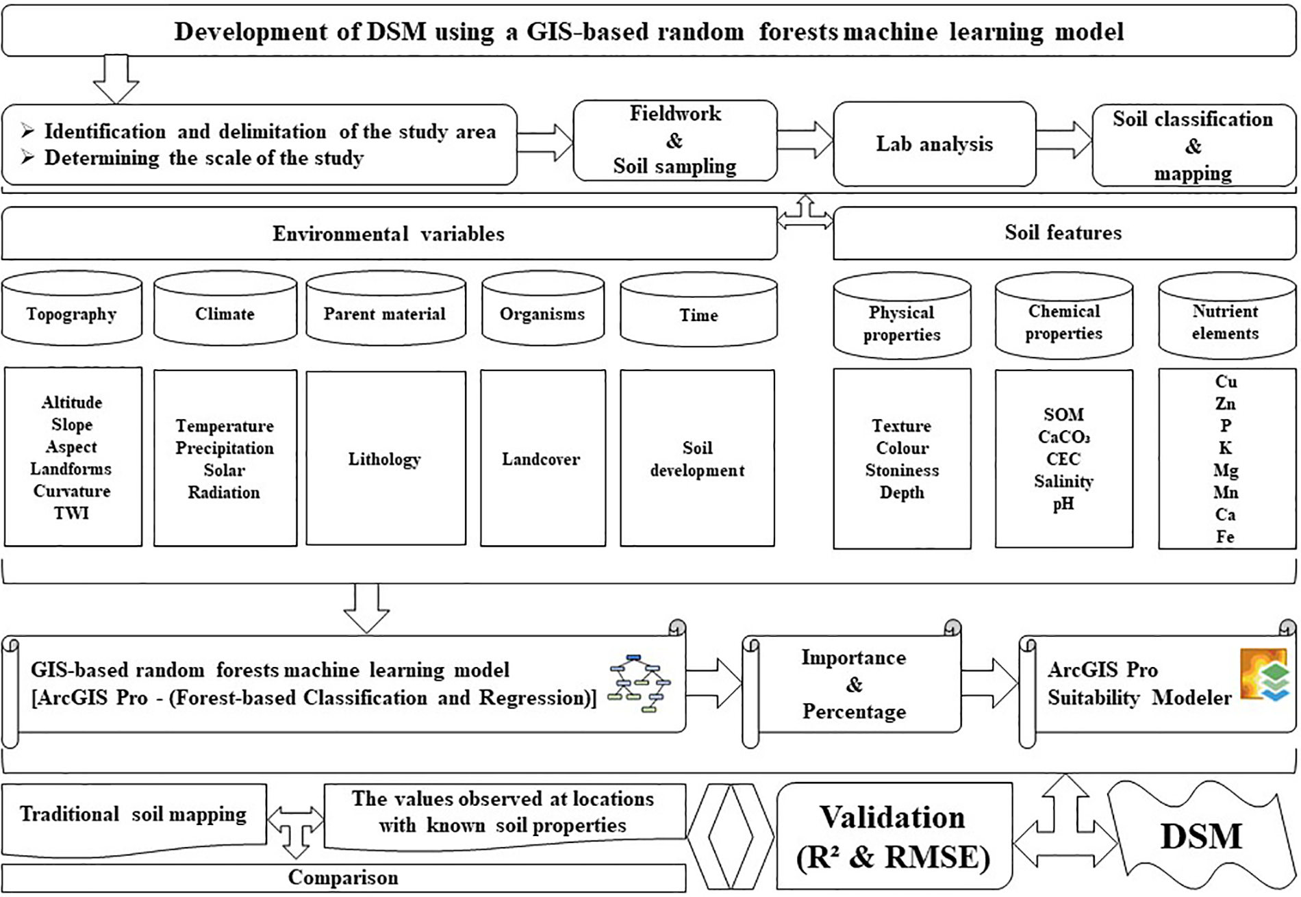
Figure 2: Methodology flowchart
Soil samples were taken according to the number of samples determined by creating 2.5 km × 2.5 km grids. Because the topography in the study area is very hilly and covered with dense vegetation, such a method was followed [54]. To cover spatial variations, 7 different locations were selected with a systematic approach. A total of 32 different samples were taken from these locations. Identification and sampling were carried out based on genetic horizons. Thus, it was aimed to understand the spatial distribution of soil types and properties of different profile layers [55]. While soil samples were taken during field studies, local data on environmental conditions were also recorded. During the DSM development phase, soil samples were organized into the topsoil (0–30 cm) and the subsoil (30–> cm) layers to be compatible with both Soil Atlas of Europe [56] data and previously reported information in the literature [57].
Soil samples were air-dried in the laboratory and then prepared for analysis by applying a series of procedures. Soil color was determined in dry and moist soil samples using the Munsell color chart [12]. Soil reaction (pH) was determined with a glass-electrode pH meter [58]. Electrical conductivity (EC) was measured with a glass-electrode EC-meter [59]. Soil texture was determined by the hydrometer method and described using the international texture triangle [60]. Lime was determined using the volumetric calcimeter method [61]. A Wheatstone Bridge concentrator measured salt in soil suspensions [62]. Soil organic matter (SOM1) was calculated according to the Modified Walkley Black Method [64]. Cation exchange capacity (CEC2) was determined by the ammonium acetate method [66]. Macro and micronutrients were determined by diethylene triamine pentaacetic acid, inductively coupled plasma (DTPA ICP), and ammonium acetate, inductively coupled plasma (AAc, ICP) extraction methods [67].
Soils in the study area were classified using Soil Taxonomy [68]. This classification was based on the spatial distribution of different soil types in the study area, soil forming factors, visual observation, and determination. The mapping of soil types and properties was carried out using GIS-based techniques. These techniques are substitutes for soil surveying and are widely used to empirically reveal the spatial distribution of key soil types and properties [69]. Thus, raster maps of the sub-variables and variables used in the DSM development were created.
The spatial distribution of soil properties in the study area was realized using the interpolation method. Inverse Distance Weighting (IDW) was determined as the most appropriate model for the distribution since its root mean square error (RMSE) is lower than other interpolation methods [70]. This estimation method assumes that the relationship between two points is directly proportional to the distance between them and the effect of the mapped variable decreases as it moves away from the sampled location [71]. Soil types in the study area were mapped using DSM or Digital Soil Assessment (DSA) techniques [72]. This model, which examines the relationship between data obtained from soil observations and auxiliary data representing the factors of soil formation, is a simplified form of the complex relationships between soil distribution patterns and variables that contribute to soil formation and development [73].
The DSM for the study area was developed in two stages. The importance of variables and soil properties (physical, chemical, and nutrients) that contribute to soil formation and development was determined in the first stage. RF algorithm was utilized, one of the most successful methods widely used in recent DSM research [74]. This algorithm is an advanced ML method to analyze high-dimensional complex data [75]. The importance ratings obtained from this algorithm were used to measure the effect of independent variables on dependent variables [76]. Thus, the importance of different factors affecting the dependent variable was easily determined [77,78]. The method used Forest-based Classification and Regression tools in ArcGIS Pro Spatial Analyst extension. During the application, importance and percentages were determined according to the decision tree created using randomly generated parts of the original (training) data (soil sample).
In another stage of DSM development, a suitability model was created to represent the distribution of soil types best. The model was applied using the ArcGIS Pro Suitability Modeler tool. For this purpose, the sub-variables whose importance levels were determined first, and then the variables were combined with the suitability model, and the DSM was obtained. DSM was grouped at the sub-group level according to soil classification results.
DSM was validated by comparing traditional soil maps [79,80] with values observed at locations with known soil properties [29,30,81]. Validation was performed based on 100 validation points randomly taken from the study area and using the coefficient of determination (R²) and RMSE, which are considered the most commonly used validation measures [82]. R² is the coefficient of determination of the model’s accuracy and a high value indicates a good prediction relationship. Since RMSE is a measure of error, a lower value indicates high performance [83]. ArcGIS Pro (Version 3.0.1) was used to apply the methods and techniques used in the study and to prepare various thematic maps.
3.1 Variables Contributing to Soil Formation and Development
Soil formation and development is a highly complex process controlled by primary (parent material, climate, topography, microorganisms, time), and subordinate variables [84,85]. Understanding this process is important for producing soil maps, often used to visualize or predict soil types and properties [86]. Therefore, soil formation and development in the study area were explained depending on the spatially mapped sub-variables of topography (landforms, aspect, slope, altitude, curvature, TWI), climate (temperature, precipitation, solar radiation), parent material (lithology), organisms (land cover) and time (soil development) factors (Table 2).
Topography was identified as the most effective (50.77%) environmental variable in the spatial distribution of soil types and properties (Table 3), because there is a clear connection between topography and soil [87]. This connection is especially strong in mountainous areas where highly different environmental conditions are observed over short distances [88]. Sub-variables of the topography were distributed as slope (12.77%), aspect (12.45%), curvature (9.27%), landforms (6.69%), altitude (6.45%) and TWI (3.14%), respectively (Table 3).
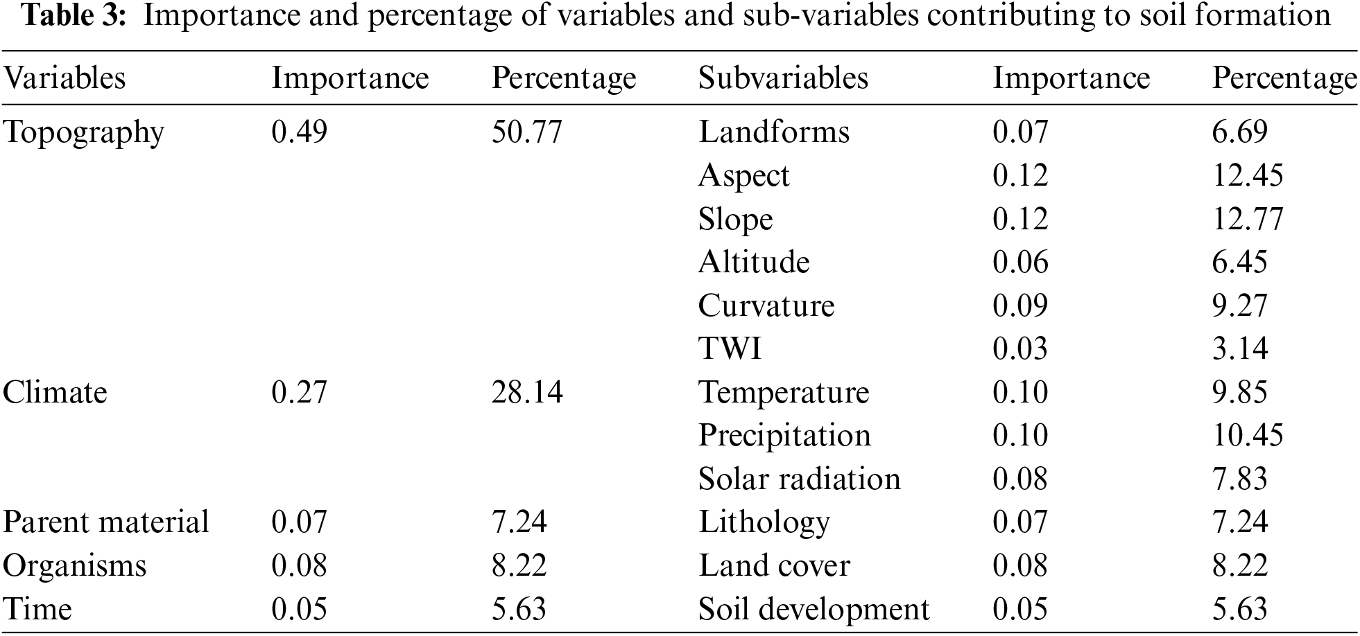
The climate was identified as another factor that has a relatively high influence on the spatial distribution of soil types and properties (28.14%). This is related to the local patterns of climate characteristics of mountainous areas and varies spatially as a function of topography and other factors [89]. Therefore, sub-variables of climate factors were distributed as precipitation (10.45%), temperature (9.85%), and solar radiation (7.83%) (Table 3).
The effect of organisms on land cover [90] and parent material on lithology [91] and the impact of time on soil development in different soils [92] were explained by sub-variables. These sub-variables played an influential role by 8.22% (land cover), 7.24% (lithology), and 5.63% (soil development), respectively (Table 3).
Morpho-dynamic processes related to high relief energy and the differences in microclimate conditions that develop accordingly contributed more to the spatial distribution of soil types and properties. Therefore, the effect of topography and climate on soil types and properties was greater than the effect of biophysical parameters.
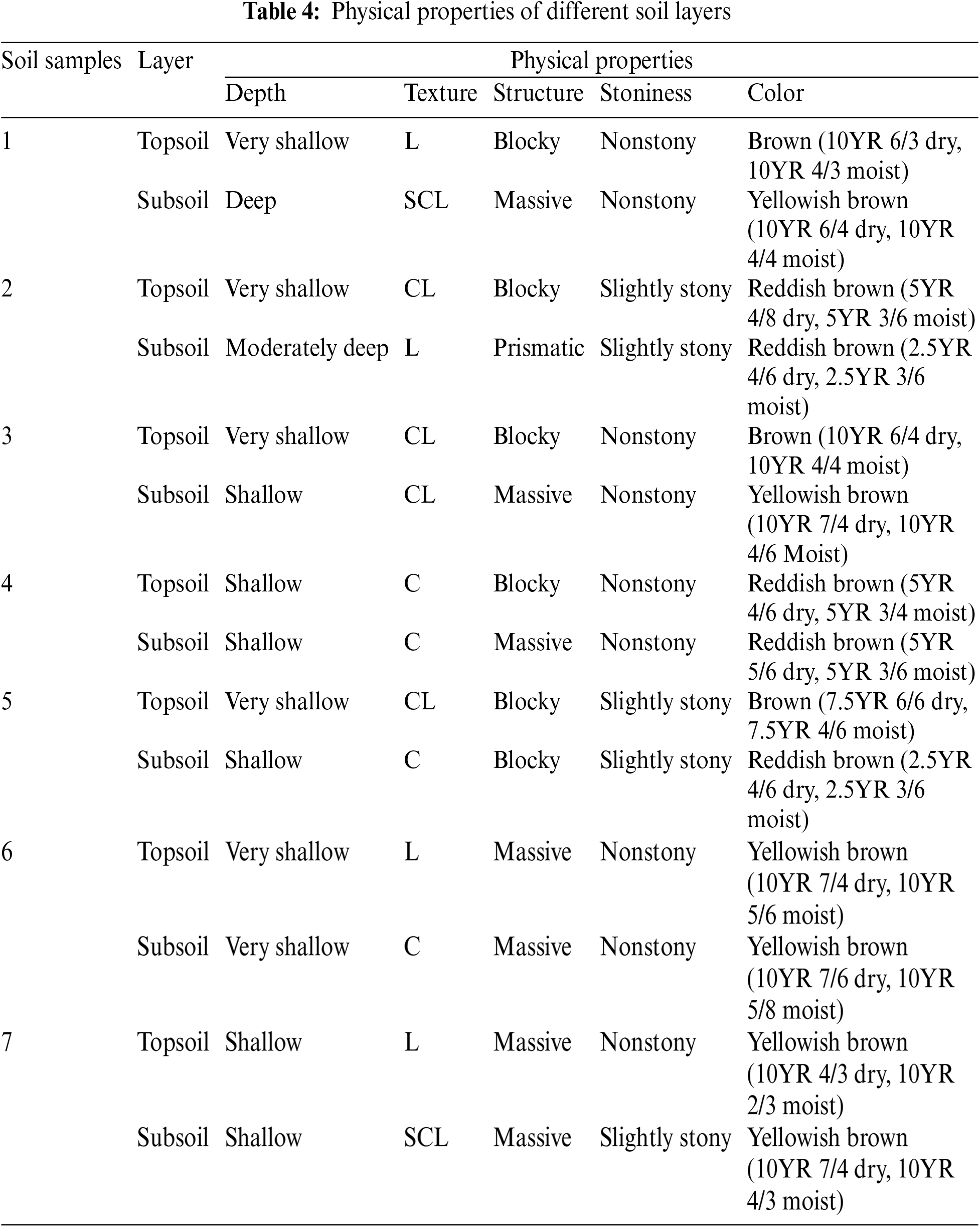
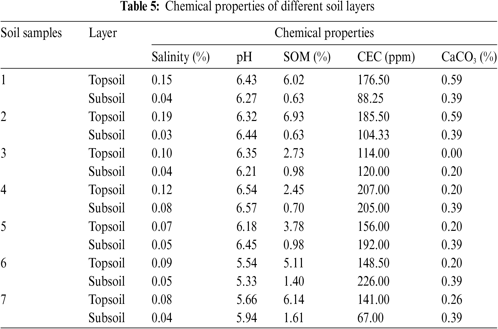
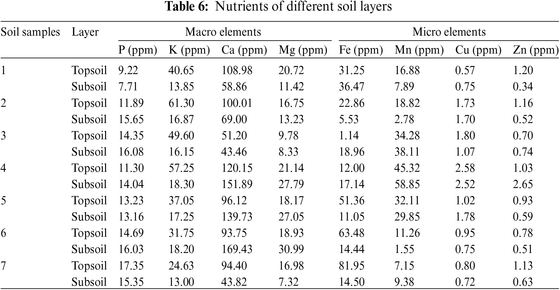
The top and subsoil layers had different physical and chemical properties and nutrients (Tables 4–6). Both were spatially different horizontally in terms of environmental factors and vertically within the layers of the soil profile.
Soil properties are interrelated at a spatial scale [93]. To analyze and interpret this relationship, the importance and percentage of the variables belonging to the properties in different soil profile layers were determined (Table 7).
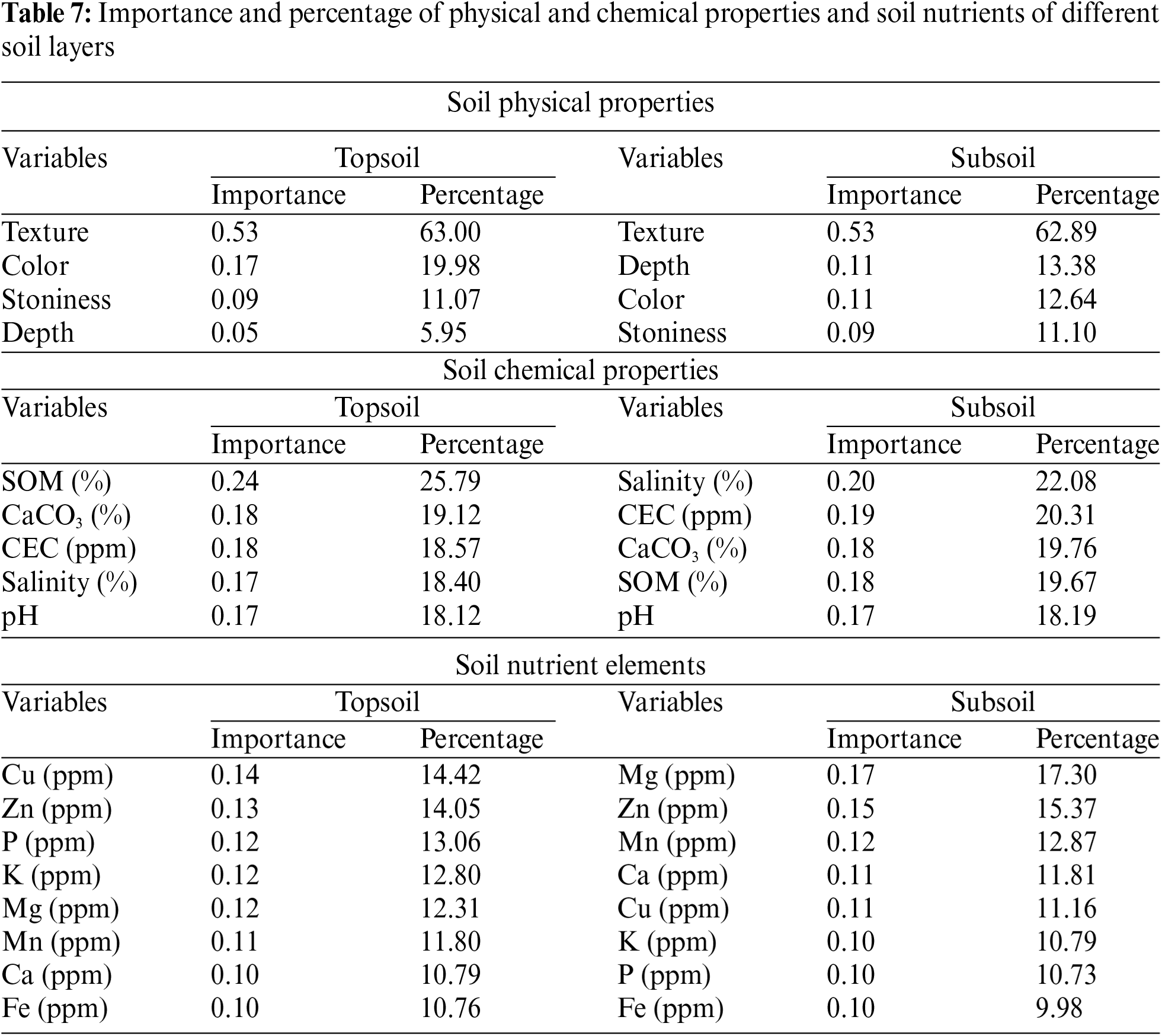
Texture was identified as the most influential variable on the physical properties of both top (63.00%) and subsoils (62.89%). Environmental factors (topography, hydrological process, and climatic conditions) and especially texture affect the spatial variation of soil physical properties [94]. Therefore, considering the importance and percentage of both parameters and the other variables, it was seen that soil physical properties exhibited a heterogeneous distribution.
SOM was identified as the most effective variable on the chemical properties of top soils (25.79%) and salinity on the chemical properties of subsoils (22.08%). SOM of topsoils should be related to the presence of forest land cover with high organic matter accumulation and the salinity of subsoils should be related to the topography and soil characteristics of the site. It was reported that SOM dynamics largely depend on land cover, climate conditions, and soil types [95], while salinity depends on landforms, land cover, soil types, and soil texture [96].
Cu (14.42%) in the topsoil and Mg (17.30%) in the subsoil were found to be the most effective variables on soil nutrients. The presence and importance of different nutrients depend mainly on the parent material [97]. Therefore, the distribution of parent material consisting of lithologies containing Cu and Mg minerals has made these minerals more important in the top and subsoils. Present soils also reflected the characteristics of bedrock. Cangir et al. [29] suggested that soils of the Strandzha Mountains show a shallow soil character with an undeveloped profile structure and physico-chemical properties and nutrients of different soil layers depend on the mineralogical structure of the sediments forming the parent material or the sequence formed by the lithological discontinuity, if any.
The remaining soil properties’ different importance and percentages are shown in Table 6. As the layers of soil profiles deepen, the significance and percentage of some variables increased while others decreased. Comparisons within and between the layers revealed that changes in soil properties were mostly realized under the influence of topography, climate, and time in topsoils and under the influence of topography, parent material, and time conditions in subsoils. Assuming the study area is relatively homogeneous in terms of organism factors related to the land cover characteristics, it was seen that soil types and properties occurred under the control of topography with the joint effect of climate, parent material, and time factors. Therefore, some environmental conditions had a more prioritized impact on the spatial distribution of soil properties of the study area.
3.3 Spatial Distribution and Mapping of Soil Types
Spatial distribution and mapping of soil types are significant for a more rational study and management of soil resources [98]. Therefore, the distribution of soil orders developed under different environmental conditions and with varying soil properties was determined. Accordingly, in the study area where only Brown Forest soils are found in the genetic system, soils belonging to Entisol, Inceptisol, and Alfisol orders were distributed (Fig. 3).
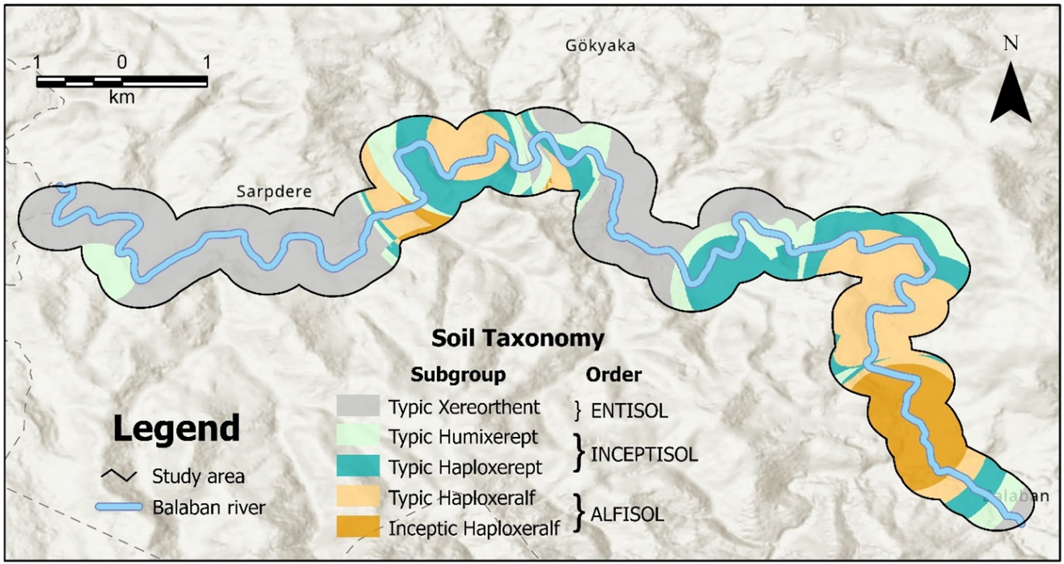
Figure 3: Soil map of the study area
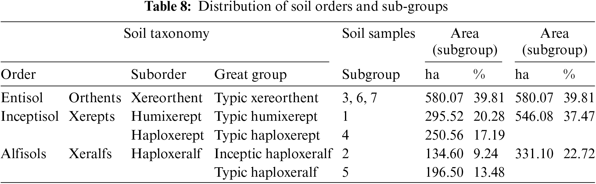
Entisols were the most widespread at the ordo level (39.81%). This is followed by Inceptisol (37.47%) and Alfisol (22.72%) soil orders from largest to smallest. Typic Xereorthent belonging to the Entisol order had the largest area at the sub-group level (Table 8). The others are listed as Typic Humixerept (20.28%), Typic Haploxerept (17.19%), Typic Haploxeralf (13.48%) and Inceptic Haploxeralf (9.24%) sub-groups, respectively (Table 8).
Validation of DSM revealed R2 as 0.66 and RMSE as 1.75. Accordingly, since the R2 value is in the range of 0.60<==R2<0.75 and the RMSE value is 1.0<RMSE<=2.0, DSM was considered to have a satisfactory performance. Therefore, the methods and techniques used in this study were proven to predict the DSM accurately.
Sustainable and functional soil management and planning require detailed information on the spatial distribution of soil types and properties [10,11]. This need is most accurately met through soil surveying, which involves field sampling, laboratory analysis, data processing, and mapping [99]. Thus, soil types and properties in a given area can be classified and a soil map can be produced to understand their spatial distribution [100]. The recent increase in demand has encouraged the production of more detailed and accurate soil maps to understand the spatial variability of soil properties [101]. DSM has emerged as an established practice [102]. This has produced detailed soil maps showing the spatial heterogeneity of soil properties consistent with the landscape [103].
DSM created with various methods such as machine learning, geostatistics and deep learning approaches based on GIS techniques has become more popular with the developments in spatial information technologies [18]. DSM provides a great advantage in mapping and monitoring soil properties in a repeatable way due to its power to show detail and a higher accuracy rate, thus it is widely used for various purposes such as decision-making and policy implementation [104]. It has also made it easier for soil scientists to make inferences to test hypotheses to understand the spatial distribution of soil types, properties, and pedogenic processes [86]. In this study, DSM was produced using the GIS-based RF method. RF was preferred because it has a higher ability to learn or accurately predict the interactions between different variables [105]. Manteghi et al. [106] found that the RF model is the best-performing model compared to other models used in the DSM generation. However, the limited number of samples available due to the study budget prevented the DSM validation result from being good to very good. Biswas et al. [101] emphasized that the sample size determined according to the available budget is of great importance as it affects the results of laboratory measurements and data analysis. They reported that care should be taken to choose the right sample size to meet the purpose of the study. Zhang et al. [12] argued that samples taken without representing the entire soil profile due to their cost may jeopardize the accuracy of the study and lead to large sampling uncertainty. On the other hand, the rugged topography of the study area also played a decisive role in limited sampling. Camera et al. [107] reported that the DSM would show lower reliability due to a lack of data based on mountainous areas’ topographical, geological, geomorphological, and climatic conditions. Gelsleichter et al. [108] reported that the DSM product will be produced with fewer samples because sampling, which can affect the spatial estimation of soil types and properties, is even more difficult in mountainous areas with limited access and transportation.
Mountainous areas are extraordinary ecosystems defined as biomes due to various environmental conditions in vertical and horizontal gradients [109]. Mountain soils distributed in these ecosystems are very important for the functioning and preserving of ecological features [88]. Since the study area has a mountain character, it has an extremely complex topography. This character of topography has played a dominant role in horizontal and vertical variation of soil properties. Therefore, the topography factor affected the spatial distribution of soil samples in the study area more dominantly. Climate factors follow this at a significant rate. Variations of local topographical features in short distances caused the climate characteristics to change. Such a case has triggered spatial differentiation of soil types and properties. Cangir et al. [29] suggested that spatial variations in topography, climate, and parent material characteristics effectively formed soil types in the Strandzha Mountains. Therefore, the study results showed that the generation of DSM using the GIS-based RF method to prepare maps of soil classes in high-relief areas helps reduce time and cost and increase accuracy. However, it was also found that the RF model, which can be used to prepare maps of soil classes in low-relief areas, is more advantageous [107].
In the last century, due to various global problems such as climate change, land use and land cover change (LUCC), deforestation, biodiversity loss, soil degradation, and erosion, studies on the spatial distribution of soil types and properties of natural landscapes have gained momentum [110]. Although only Brown Forest soils were distributed in the genetic system in the present study area, some other soil groups belonging to Entisol, Inceptisol, and Alfisol orders existed. Such a case was because only soil formation factors in the genetic system are considered in classifying soil types. In contrast, soil properties and morphology are considered in soil taxonomy [111].
In the study area, the most common soil type was found to be Entisol. Dinç et al. [112] reported that Entisols, one of the most widespread soil orders in Türkiye and the Thracian Peninsula, occur on sloping lands of mountainous or newly deposited areas. Cangir et al. [29] reported that entisols are encountered in the forested regions of the Strandzha Mountains, especially near river beds. On the other hand, the second dominant soil order of the study area was identified as Inceptisols. Haktanır et al. [113] suggested that Inceptisols are the most commonly observed soil order in Türkiye after Entisols.
Mountainous areas, which form a special ecosystem compared to their surroundings, have a complex and fragile ecosystem. Soils in these special ecosystems are highly dynamic systems that can respond more sensitively to environmental changes. Therefore, assessing and mapping the spatial distribution of the types and characteristics of mountain soils is crucial for a better understanding of the orobiomes of our planet. This study used a GIS-based RF machine-learning model to estimate spatial variability of soil types and properties under forest cover of the Strandzha Mountains of Türkiye. For this purpose, environmental factors and soil properties affecting soil formation and development were analyzed. DSM was developed for the study area by associating the findings with the soil survey results. DSM suggests that the factors affecting the spatial distribution of soil types and properties in the sample area are, from most important to least important, topography (50.77%), climate (28.14%), organisms (8.22%), parent material (7.24%) and time (5.63%). With the contributions of all these factors at different rates, it was determined that Entisols were the most widespread in the study area at the ordo level (39.81%). The other soil orders, Inceptisol (37.47%) and Alfisol (22.72%) have a smaller spatial distribution. Present findings may be useful in making inferences about the spatial distribution of soil types and properties of similar landscapes and explaining the factors affecting this distribution. It was also concluded that the number of samples should be increased to obtain more reliable results from DSM. However, it was confirmed that a GIS-based RF machine learning model could reliably be used to produce DSM.
Acknowledgement: This study did not receive public and commercial funding support from agencies.
Funding Statement: This study was funded by the Scientific Research Projects Coordination Unit of Tekirdag Namık Kemal University. Project Number: NKUBAP.03.YLGA.21.324.
Author Contributions: The authors confirm contribution to the paper as follows: Emre Ozsahin: Conceived and designed the analysis, collected the data, and performed the analysis; Huseyin Sarı: Grant recipient, collected the data & other contributions; Duygu Boyraz Erdem: Contributed data and analysis, wrote the paper & other contributions; Mikail Ozturk: Survey data collection & other contributions. All authors reviewed the results and approved the final version of the manuscript.
Availability of Data and Materials: Data will be made available on request.
Ethics Approval: Not applicable.
Conflicts of Interest: The authors declare they have no conflicts of interest to report regarding the present study.
1Soil organic matter (SOM) is the organic material found in soil [63].
2Cation exchange capacity (CEC) measures the soil’s ability to hold positively charged ions [65].
References
1. Ghavami MS, Ayoubi S, Mosaddeghi MR, Naimi S. Digital mapping of soil physical and mechanical properties using machine learning at the watershed scale. J Mt Sci. 2023;20(10):2975–92. doi:10.1007/s11629-023-8056-z. [Google Scholar] [CrossRef]
2. Shakir KM, Suhail M, Alharbi T. Evaluation of urban growth and land use transformation in Riyadh using Landsat satellite data. Arab J Geosci. 2018;11(18):540. doi:10.1007/s12517-018-3896-5. [Google Scholar] [CrossRef]
3. Sarı H, Özşahin E. Evaluation of soil properties of Tekirdag province using GIS (geoinformation systems) and DSM (digital soil mapping) techniques. In: Ahi Evran International Conference on Scientific Research, 2022 Oct 21–23, 2022; Kirsehir, Türkiye: Iksad Publications; p. 81–96. [Google Scholar]
4. Suleymanov A, Tuktarova I, Belan L, Suleymanov R, Gabbasova I, Araslanova L. Spatial prediction of soil properties using random forest, k-nearest neighbors and cubist approaches in the foothills of the Ural mountains. Russia Model Earth Syst Environ. 2023;9(3):3461–71. doi:10.1007/s40808-023-01723-4. [Google Scholar] [CrossRef]
5. Song X, Guo J, Wang X, Du Z, Ren R, Lu S, et al. Afforestation alters the molecular composition of soil organic matter in the central loess plateau of China. Forests. 2023;14(7):1502. doi:10.3390/f14071502. [Google Scholar] [CrossRef]
6. Labouyrie M, Ballabio C, Romero F, Panagos P, Jones A, Schmid MW, et al. Patterns in soil microbial diversity across Europe. Nat Commun. 2023;14(1):3311. doi:10.1038/s41467-023-37937-4. [Google Scholar] [PubMed] [CrossRef]
7. Li Y, Ma J, Li Y, Jia Q, Shen X, Xia X. Spatiotemporal variations in the soil quality of agricultural land and its drivers in China from 1980 to 2018. Sci Total Environ. 2023;892:164649. doi:10.1016/j.scitotenv.2023.164649. [Google Scholar] [PubMed] [CrossRef]
8. Bhunia GS, Shit PK, Maiti R. Comparison of GIS-based interpolation methods for the spatial distribution of soil organic carbon (SOC). J Saudi Soc Agric Sci. 2018;17(2):114–26. doi:10.1016/j.jssas.2016.02.001. [Google Scholar] [CrossRef]
9. Özaytekin HH, Dedeoğlu M. Weathering rates and mass balance of soils developed on Hasandag volcanic materials. Anadolu J Agric Sci. 2021;36(1):81–92. doi:10.7161/omuanajas.789497. [Google Scholar] [CrossRef]
10. Barthold FK, Wiesmeier M, Breuer L, Frede HG, Wu J, Blank FB. Land use and climate control the spatial distribution of soil types in the grasslands of Inner Mongolia. J Arid Environ. 2013;88:194–205. doi:10.1016/j.jaridenv.2012.08.004. [Google Scholar] [CrossRef]
11. Han P, Dong D, Zhao X, Jiao L, Lang Y. A smartphone-based soil color sensor: for soil type classification. Comput Electron Agric. 2016;123(7):232–41. doi:10.1016/j.compag.2016.02.024. [Google Scholar] [CrossRef]
12. Zhang Y, Hartemink AE, Huang J, Minasny B. Digital soil morphometrics. Encycl Soils Environ (Second Ed). 2023;4:568–78. doi:10.1016/B978-0-12-822974-3.00008-2. [Google Scholar] [CrossRef]
13. Ajami M, Heidari A, Khormali F, Gorji M, Ayoubi S. Environmental factors controlling soil organic carbon storage in loess soils of a subhumid region, northern Iran. Geoderma. 2016;281(6):1–10. doi:10.1016/j.geoderma.2016.06.017. [Google Scholar] [CrossRef]
14. Fox EW, Hoef JMV, Olsen AR. Comparing spatial regression to random forests for large environmental data sets. PLoS One. 2020;15(3):e0229509. doi:10.1371/journal.pone.0229509. [Google Scholar] [PubMed] [CrossRef]
15. Saha A, Basu S, Datta A. Random forests for spatially dependent data. J Am Stat Assoc. 2021;118(541):665–83. doi:10.1080/01621459.2021.1950003. [Google Scholar] [CrossRef]
16. Khan K, Calder CA. Restricted spatial regression methods: implications for ınference. J Am Stat Assoc. 2022;117(537):482–94. doi:10.1080/01621459.2020.1788949. [Google Scholar] [PubMed] [CrossRef]
17. Garosi Y, Ayoubi S, Nussbaum M, Sheklabadi M. Effects of different sources and spatial resolutions of environmental covariates on predicting soil organic carbon using machine learning in a semi-arid region of Iran. Geoderma Reg. 2022;29(2):e00513. doi:10.1016/j.geodrs.2022.e00513. [Google Scholar] [CrossRef]
18. Matazi AK, Gognet EE, Kakaï RG. Digital soil mapping: a predictive performance assessment of spatial linear regression, Bayesian and ML-based models. Model Earth Syst Environ. 2023;10(1):595–61. doi:10.1007/s40808-023-01788-1. [Google Scholar] [CrossRef]
19. Mansuy N, Thiffault E, Paré D, Bernier P, Guindon L, Villemaire P, et al. Digital mapping of soil properties in canadian managed forests at 250 m of resolution using the k-nearest neighbor method. Geoderma. 2014;235:59–73. doi:10.1016/j.geoderma.2014.06.032. [Google Scholar] [CrossRef]
20. Ottoy S, De Vos B, Sindayihebura A, Hermy M, Van Orshoven J. Assessing soil organic carbon stocks under current and potential forest cover using digital soil mapping and spatial generalization. Ecol Indic. 2017;77:139–50. doi:10.1016/j.ecolind.2017.02.010. [Google Scholar] [CrossRef]
21. Chen L, Ren C, Li L, Wang Y, Zhang B, Wang Z, et al. A comparative assessment of geostatistical, machine learning, and hybrid approaches for mapping topsoil organic carbon content. ISPRS Int J Geoinf. 2019;8(4):174. doi:10.3390/ijgi8040174. [Google Scholar] [CrossRef]
22. Entezari M, Ayoubi S, Karimi A, Naimi S. Digital exploration of selected heavy metals using random forest and a set of environmental covariates at the watershed scale. J Hazard Mater. 2023;455(4):131609. doi:10.1016/j.jhazmat.2023.131609. [Google Scholar] [PubMed] [CrossRef]
23. Bahri H, Raclot D, Barbouchi M, Lagacherie P, Annabi M. Mapping soil organic carbon stocks in tunisian topsoils. Geoderma Reg. 2022;30(8):e00561. doi:10.1016/j.geodrs.2022.e00561. [Google Scholar] [CrossRef]
24. Kaya F, Keshavarzi A, Francaviglia R, Kaplan G, Başayiğit L, Dedeoğlu M. Assessing machine learning-based prediction under different agricultural practices for digital mapping of soil organic carbon and available phosphorus. Agriculture. 2022;12(7):1062. doi:10.3390/agriculture12071062. [Google Scholar] [CrossRef]
25. Dolatabadi N, Nasseri M, Zahraie B. Comparative assessment of surface soil moisture simulations by the coupled wcm-iem vs. data-driven models using the sentinel 1 and 2 satellite images. Earth Sci Inform. 2023;16(2):1563–84. doi:10.1007/s12145-023-00987-9. [Google Scholar] [CrossRef]
26. Fantappiè M, L’Abate G, Schillaci C, Costantini EAC. Digital soil mapping of Italy to map derived soil profiles with neural networks. Geoderma Reg. 2023;32(2):e00619. doi:10.1016/j.geodrs.2023.e00619. [Google Scholar] [CrossRef]
27. Padarian J, Minasny B, McBratney AB. Machine learning and soil sciences: a review aided by machine learning tools. Soil. 2020;6(1):35–52. doi:10.5194/soil-6-35-2020. [Google Scholar] [CrossRef]
28. Poggio L, Gimona A, Spezia L, Brewer MJ. Bayesian spatial modelling of soil properties and their uncertainty: the example of soil organic matter in Scotland using R-INLA. Geoderma. 2016;277(20):69–82. doi:10.1016/j.geoderma.2016.04.026. [Google Scholar] [CrossRef]
29. Cangir C, Boyraz D. Yıldız Orman Ekosisteminde Yer Alan Tipik Toprakların Sınıflandırılması ve Amenajmanları. Tekirdağ Ziraat Fakültesi Dergisi. 2009;6(1):65–77 (In Turkish). [Google Scholar]
30. Sevgi O. Soil characteristics of different sites in Strandzha (Yildiz) mountain. Challenges of establishment and management of a trans-border biosphere reserve between Bulgaria and Turkey in Strandzha mountain. In: Proceedings of a UNESCO-BAS-MOEW Workshop, 2005 Nov 11–13; Bourgas, Bulgaria; p. 77–86. 2005. Available from: https://www.cabdirect.org/cabdirect/FullTextPDF/2008/20083240801.pdf. [Accessed 2024]. [Google Scholar]
31. Iliev I, Ilieva Z. Soil nematodes of family plectidae (Nematoda, Plectida) in different plant communities in Strandzha mountain (Bulgaria, Turkey). Silva Balc. 2016;17(1):71–108. Available from: https://www.cabdirect.org/cabdirect/FullTextPDF/2016/20163391384.pdf. [Accessed 2024]. [Google Scholar]
32. Malinova L, Petrova K, Grigorova-Pesheva B. Lixisols and Acrisols on the territory of Strandzha Mountain. Bulg J Agric Sci. 2021;27(1):179–85. Available from: https://www.agrojournal.org/27/01-24.pdf. [Accessed 2024]. [Google Scholar]
33. Shishkov T, Dimitrov E. Diagnostic of soil forming processes of Zheltozem podzolic (pseudopodzolic) soils from Strandzha mountain. Bulg J Agric Sci. 2022;28(2):318–23. Available from: https://www.agrojournal.org/28/02-18.pdf. [Accessed 2024]. [Google Scholar]
34. Kantarcı MD. Analytical investigation of eluviation and accumulation horizons of soils formed on silicate parent material under temperate climate conditions. J Fac For Istanb Univ. 1979;29(1):14–53. Available from: https://dergipark.org.tr/tr/pub/jffiu/issue/18696/197211. [Accessed 2024]. [Google Scholar]
35. Sevgi O. Properties of soil which is under the forest and clear cutter areas in the forest at granite land of Demirköy (Master Thesis). Istanbul University Institute of Science and Technology: Istanbul; 1993. [Google Scholar]
36. Makinacı E. The ecological investigation of rejuvenation methods in Demirköy Oak forests (Master Thesis). Istanbul University Institute of Science and Technology: Istanbul; 1993. [Google Scholar]
37. Deniz M. The researches about the afforestation areas of crimean pine and sctch pine in Demirköy (Master Thesis). Istanbul University Institute of Science and Technology: Istanbul; 1993. [Google Scholar]
38. Plotnikova OO, Romanis TV, Kust PG. Comparison of digital image analysis methods for morphometric characterization of soil aggregates in thin sections. Dokuchaev Soil Bull. 2020;104(104):199–222. doi:10.19047/0136-1694-2020-104-199-222. [Google Scholar] [CrossRef]
39. Assami T, Hamdi-Aїssa B. Digital mapping of soil classes in Algeria—a comparison of methods. Geoderma Reg. 2019;16(240):e00215. doi:10.1016/j.geodrs.2019.e00215. [Google Scholar] [CrossRef]
40. Matinfar HR, Maghsodi Z, Mousavi SR, Rahmani A. Evaluation and prediction of topsoil organic carbon using machine learning and hybrid models at a field-scale. Catena. 2021;202(3–4):105258. doi:10.1016/j.catena.2021.105258. [Google Scholar] [CrossRef]
41. Taghizadeh-Mehrjardi R, Schmidt K, Toomanian N, Heung B, Behrens T, Mosavi A, et al. Improving the spatial prediction of soil salinity in arid regions using wavelet transformation and support vector regression models. Geoderma. 2021;383(189):114793. doi:10.1016/j.geoderma.2020.114793. [Google Scholar] [CrossRef]
42. Singh R, Tiwari AK, Singh GS. Managing riparian zones for river health improvement: an integrated approach. Landsc Ecol Eng. 2021;17(2):195–223. doi:10.1007/s11355-020-00436-5. [Google Scholar] [CrossRef]
43. Maruani T, Amit-Cohen I. The effectiveness of the protection of riparian landscapes in Israel. Land Use Policy. 2009;26(4):911–8. doi:10.1016/j.landusepol.2008.11.002. [Google Scholar] [CrossRef]
44. Angiolini C, de Simone L, Fiaschi T, Cifaldi GP, Maccherini S, Fanfarillo E. Detecting the imprints of past clear-cutting on riparian forest plant communities along a Mediterranean river. River Res Appl. 2023;39(8):1–13. doi:10.1002/rra.4152. [Google Scholar] [CrossRef]
45. MTA. Geological maps of Turkey. General directorate of mineral research and exploration. Ankara. Turkey: General Directorate of Mineral Research and Exploration-MTA; 2002. [Google Scholar]
46. GDM. DEM (digital elevation model) (resolution: 5 m) data, digital surface model 5 m level-0 (SYM5-L. 2023, HGM (general directorate of mapping), Ankara; 2023. Available from: https://www.harita.gov.tr/urun/sayisal-yuzey-modeli-5-m-seviye-0-sym5-l0-/1. [Accessed 2024]. [Google Scholar]
47. Yılmaz E, Çiçek İ. Detailed Köppen-Geiger climate regions of Turkey. J Hum Sci. 2018;15(1):225–42. doi:10.14687/jhs.v15i1.5040. [Google Scholar] [CrossRef]
48. Dönmez Y. Vegetation geography of the Thracian peninsula. Istanbul: Istanbul University, Geography Institute Publications; 1990. [Google Scholar]
49. Zanaga D, Van De Kerchove R, Daems D, De Keersmaecker W, Brockmann C, Kirches G, et al. ESA WorldCover 10 m 2021 v200. 2022. doi:10.5281/zenodo.7254221. [Google Scholar] [CrossRef]
50. ESA. The ESA WorldCover 10 m 2021 V200 product. 2023. Available from: https://worldcover2021.esa.int/downloader. [Accessed 2024]. [Google Scholar]
51. Fick SE, Hijmans RJ. WorldClim 2: new 1-km spatial resolution climate surfaces for global land areas. Int J Climatol. 2017;37(12):4302–15. doi:10.1002/joc.5086. [Google Scholar] [CrossRef]
52. WorldClim. WorldClim—global climate data. 2019. Available from: www.worldclim.org. [Accessed 2024]. [Google Scholar]
53. Moore ID, Grayson RB, Ladson AR. Digital terrain modelling: a review of hydrological, geomorphological, and biological applications. Hydrol Process. 1991;5(1):3–30. doi:10.1002/hyp.3360050103. [Google Scholar] [CrossRef]
54. Jiang L. A fast and accurate circle detection algorithm based on random sampling. Future Gener Comput Syst. 2021;123(1):245–56. doi:10.1016/j.future.2021.05.010. [Google Scholar] [CrossRef]
55. Andersson H, Bergström L, Djodjic F, Ulén B, Kirchmann H. Topsoil and subsoil properties influence phosphorus leaching from four agricultural soils. J Environ Qual. 2013;42(2):455–63. doi:10.2134/jeq2012.0224. [Google Scholar] [PubMed] [CrossRef]
56. European Communities. Soil atlas of Europe. European Soil Bureau Network European Commission. Luxembourg: Office for Official Publications of the European Communities; 2005. p. 128. [Google Scholar]
57. Wadoux AMJC, Padarian J, Minasny B. Multi-source data integration for soil mapping using deep learning. Soil. 2019;5(1):107–19. doi:10.5194/soil-5-107-2019. [Google Scholar] [CrossRef]
58. Jackson ML. Soil chemical analysis. Englewood Cliffs, NJ: Prentice-Hall Inc.; 1958. p. 498. [Google Scholar]
59. Black CA. Methods of soil analysis: part I, physical and mineralogical properties. Madison, Wisconsin: American Society of Agronomy; 1965. [Google Scholar]
60. Soil Survey Division Staff. Soil survey manual. Soil conservation service. In: US Department of Agriculture handbook 18. USA: Soil Conservation Service (SCS); 1993. [Google Scholar]
61. Sağlam MT. Toprak ve Suyun Kimyasal Analiz Yöntemleri. Trakya Üniversitesi Tekirdağ: Namık Kemal Üniversitesi Ziraat Fakültesi Yayınları; 1994. [Google Scholar]
62. Richards LA. Diagnosis and improvement of saline and alkali soils. In: Agricultural hand book 60. Washington, DC, USA: U.S. Department of Agriculture; 1954. [Google Scholar]
63. Chenu C, Rumpel C, Védère C, Barré P. Chapter 13—methods for studying soil organic matter: nature, dynamics, spatial accessibility, and interactions with minerals. Soil Microbiol, Ecol Biochem (Fifth Ed). 2024;2(7):369–406. doi:10.1016/B978-0-12-822941-5.00013-2. [Google Scholar] [CrossRef]
64. Walkley A. A critical examination of a rapid method for determining organic carbon in soils: effect of variations in digestion conditions and of inorganic soil constituents. Soil Sci. 1947;63(4):251–64. doi:10.1097/00010694-194704000-00001. [Google Scholar] [CrossRef]
65. Yadav SP, Bhandari S, Bhatta D, Poudel A, Bhattarai S, Yadav P, et al. Biochar application: a sustainable approach to improve soil health. J Agric Food Res. 2023;11:100498. doi:10.1016/j.jafr.2023.100498. [Google Scholar] [CrossRef]
66. Lewis DR. Analytical data on reference clay materials. In: A.P.I. research project 49, preliminary report no. 7. New York, NY, USA: Columbia University; 1949. [Google Scholar]
67. Rauret G. Extraction procedures for the determination of heavy metals in contaminated soil and sediment. Talanta. 1998;46(3):449–455. doi:10.1016/s0039-9140(97)00406-2. [Google Scholar] [PubMed] [CrossRef]
68. Soil Survey Staff Keys to Soil Taxonomy. Soil survey staff keys to soil taxonomy. In: Soil survey staff keys to soil taxonomy. 13th ed. Washington, DC, USA: U.S. Department of Agriculture, Natural Resources Conservation Service; 2022. [Google Scholar]
69. Rahbar Alam Shirazi F, Shahbazi F, Rezaei H, Biswas A. Digital assessments of soil organic carbon storage using digital maps provided by static and dynamic environmental covariates. Soil Use Manag. 2023;39(2):948–74. doi:10.1111/sum.12900. [Google Scholar] [CrossRef]
70. Chen C, Zhao N, Yue T, Guo J. A generalization of inverse distance weighting method via kernel regression and its application to surface modeling. Arab J Geosci. 2015;8(9):6623–33. doi:10.1007/s12517-014-1717-z. [Google Scholar] [CrossRef]
71. Hama Rash AJ, Khodakarami L, Muhedin DA, Hamakareem MI, Hama Ali HF. Spatial modeling of geotechnical soil parameters: integrating ground-based data, RS technique, spatial statistics and GWR model. J Eng Res. 2024;12(1):75–85. doi:10.1016/j.jer.2023.10.026. [Google Scholar] [CrossRef]
72. Bel-Lahbib S, Ibno Namr K, Rerhou B, Mosseddaq F, El Bourhrami B, Moughli L. Assessment of soil quality by modeling soil quality index and mapping soil parameters using IDW interpolation in Moroccan semi-arid. Model Earth Syst Environ. 2023;9(4):4135–53. doi:10.1007/s40808-023-01718-1. [Google Scholar] [CrossRef]
73. Rostaminia M, Rahmani A, Mousavi SR, Taghizadeh-Mehrjardi R, Maghsodi Z. Spatial prediction of soil organic carbon stocks in an arid rangeland using machine learning algorithms. Environ Monit Assess. 2021;193(12):1–17. doi:10.1007/s10661-021-09543-8. [Google Scholar] [PubMed] [CrossRef]
74. Breiman L. Random forests. Mach Learn. 2001;45(1):5–32. doi:10.1023/A:1010933404324. [Google Scholar] [CrossRef]
75. Zeraatpisheh M, Ayoubi S, Jafari A, Finke P. Comparing the efficiency of digital and conventional soil mapping to predict soil types in a semi-arid region in Iran. Geomorphol. 2017;285(1):186–204. doi:10.1016/j.geomorph.2017.02.015. [Google Scholar] [CrossRef]
76. Jin Y, Liu X, Chen Y, Liang X. Land-cover mapping using random forest classification and incorporating NDVI time-series and texture: a case study of central Shandong. Int J Remote Sens. 2018;39(23):8703–23. doi:10.1080/01431161.2018.1490976. [Google Scholar] [CrossRef]
77. Huang L, Shahtahmassebi A, Gan M, Deng J, Wang J, Wang K. Characterizing spatial patterns and driving forces of expansion and regeneration of industrial regions in the Hangzhou megacity, China. J Clean Prod. 2020;253:119959. doi:10.1016/j.jclepro.2020.119959. [Google Scholar] [CrossRef]
78. Ma J, Cheng JCP, Jiang F, Chen W, Zhang J. Analyzing driving factors of land values in urban scale based on big data and non-linear machine learning techniques. Land Use Policy. 2020;94(1):104537. doi:10.1016/j.landusepol.2020.104537. [Google Scholar] [CrossRef]
79. Topraksu. Inventory map of Kırklareli province. Ankara: Ministry of Rural Affairs, General Directorate of Topraksu. Soil Surveys and Mapping Department, Land Classification Branch. 1972. Ministry Publications. 165. General Directorate Publications. 249. Reports Series: 37; 1972. [Google Scholar]
80. Kapur S, Akça E, Günal H. The soils of Turkey. Switzerland: Springer International Publishing AG; 2018. doi:10.1007/978-3-319-64392-2. [Google Scholar] [CrossRef]
81. Piikki K, Wetterlind J, Söderström M, Stenberg B. Perspectives on validation in digital soil mapping of continuous attributes—a review. Soil Use Manag. 2021;37(1):7–21. doi:10.1111/sum.12694. [Google Scholar] [CrossRef]
82. Schmidinger J, Heuvelink GBM. Validation of uncertainty predictions in digital soil mapping. Geoderma. 2023;437(2):116585. doi:10.1016/j.geoderma.2023.116585. [Google Scholar] [CrossRef]
83. Gültepe Y. A comparative assessment on air pollution estimation by machine learning algorithms. Eur J Sci Technol. 2019;16:8–15. doi:10.31590/ejosat.530347. [Google Scholar] [CrossRef]
84. Jenny H. Factors of soil formation: A system of quantitative pedology. New York: Dover Publications; 1941. [Google Scholar]
85. Johnson WM. The pedon and the polypedon. Soil Sci Soc Am J. 1963;27(2):212–5. doi:10.2136/sssaj1963.03615995002700020034x. [Google Scholar] [CrossRef]
86. Kebonye NM, Agyeman PC, Seletlo Z, Eze PN. On exploring bivariate and trivariate maps as visualization tools for spatial associations in digital soil mapping: a focus on soil properties. Precis Agric. 2023;24(2):511–32. doi:10.1007/s11119-022-09955-7. [Google Scholar] [CrossRef]
87. Schaetzl RJ, Anderson S. Soils: genesis and geomorphology. UK: Cambridge University Press; 2005. Available from: https://www.geokniga.org/bookfiles/geokniga-schaetzlsoils2005.pdf. [Accessed 2024]. [Google Scholar]
88. Egli M, Poulenard J. Soils of mountainous landscape. In: Richardson D, Castree N, Goodchild MF, Kobayashi A, Liu W, Marston RA, editors. International encyclopedia of geography: people, the earth, environment and technology. USA: Wiley-Blackwell; 2016. doi:10.1002/9781118786352.wbieg0197. [Google Scholar] [CrossRef]
89. Fathololoumi S, Vaezi AR, Alavipanah SK, Ghorbani A, Biswas A. Comparison of spectral and spatial-based approaches for mapping the local variation of soil moisture in a semi-arid mountainous area. Sci Total Environ. 2020;724:138319. doi:10.1016/j.scitotenv.2020.138319. [Google Scholar] [PubMed] [CrossRef]
90. Kooch Y, Ehsani S, Akbarinia M. Stratification of soil organic matter and biota dynamics in natural and anthropogenic ecosystems. Soil Tillage Res. 2020;200:104621. doi:10.1016/j.still.2020.104621. [Google Scholar] [CrossRef]
91. Gray M, Bishop TFA, Wilford JR. Lithology and soil relationships for soil modelling and mapping. Catena. 2016;147(8):429–40. doi:10.1016/j.catena.2016.07.045. [Google Scholar] [CrossRef]
92. Huggett RJ. Soil chronosequences, soil development, and soil evolution: a critical review. Catena. 1998;32(3–4):155–72. doi:10.1016/S0341-8162(98)00053-8. [Google Scholar] [CrossRef]
93. Iqbal J, Thomasson JA, Jenkins JN, Owens PR, Whisler FD. Spatial variability analysis of soil physical properties of alluvial soils. Soil Sci Soc Am J. 2005;69(4):1338–50. doi:10.2136/sssaj2004.0154. [Google Scholar] [CrossRef]
94. Yang F, An F, Ma H, Wang Z, Zhou X, Liu Z. Variations on soil salinity and sodicity and its driving factors analysis under microtopography in different hydrological conditions. Water. 2016;8(6):227. doi:10.3390/w8060227. [Google Scholar] [CrossRef]
95. Kunlanit B, Khwanchum L, Vityakon P. Land use changes affecting soil organic matter accumulation in topsoil and subsoil in northeast Thailand. Appl Environ Soil Sci. 2020;2020(1):8241739. doi:10.1155/2020/8241739. [Google Scholar] [CrossRef]
96. Yu J, Li Y, Han G, Zhou D, Fu Y, Guan B, et al. The spatial distribution characteristics of soil salinity in coastal zone of the yellow river delta. Environ Earth Sci. 2014;72(2):589–99. doi:10.1007/s12665-013-2980-0. [Google Scholar] [CrossRef]
97. Bolat İ, Kara Ö. Plant nutrients: sources, functions, deficiencies and redundancy. J Bartin Fac For. 2017;19(1):218–28. Available from: https://dergipark.org.tr/tr/pub/barofd/issue/27137/251313. [Accessed 2024]. [Google Scholar]
98. Shi XZ, Yu DS, Warner ED, Sun WX, Petersen GW, Gong ZT, et al. Cross-reference system for translating between genetic soil classification of China and soil taxonomy. Soil Sci Soc Am J. 2006;70(1):78–83. doi:10.2136/sssaj2004.0318. [Google Scholar] [CrossRef]
99. McBratney AB, Odeh IOA, Bishop TFA, Dunbar MS, Shatar TM. An overview of pedometric techniques for use in soil survey. Geoderma. 2000;97(3–4):293–327. doi:10.1016/S0016-7061(00)00043-4. [Google Scholar] [CrossRef]
100. McBratney AB, Mendonça-Santos ML, Minasny B. On digital soil mapping. Geoderma. 2003;117(1–2):3–52. doi:10.1016/S0016-7061(03)00223-4. [Google Scholar] [CrossRef]
101. Biswas A, Zhang Y. Sampling designs for validating digital soil maps: a review. Pedosphere. 2018;28(1):1–15. doi:10.1016/S1002-0160(18)60001-3. [Google Scholar] [CrossRef]
102. Nussbaum N, Zimmermann S, Walthert L, Baltensweiler A. Benefits of hierarchical predictions for digital soil mapping–an approach to map bimodal soil pH. Geoderma. 2023;437(21):116579. doi:10.1016/j.geoderma.2023.116579. [Google Scholar] [CrossRef]
103. Rosemary F, Vitharana UWA, Indraratne SP, Weerasooriya R, Mishra U. Exploring the spatial variability of soil properties in an Alfisol soil catena. Catena. 2017;150(5):53–61. doi:10.1016/j.catena.2016.10.017. [Google Scholar] [CrossRef]
104. Richer-de-Forges AC, Chen Q, Baghdadi N, Chen S, Gomez C, Jacquemoud S, et al. Remote sensing data for digital soil mapping in French research—a review. Remote Sens. 2023;15(12):3070. doi:10.3390/rs15123070. [Google Scholar] [CrossRef]
105. Llewelyn J, Strona G, Dickman CR, Greenville AC, Wardle GM, Lee MSY, et al. Predicting predator-prey interactions in terrestrial endotherms using random forest. Ecography. 2023;2023(9):e06619. doi:10.1111/ecog.06619. [Google Scholar] [CrossRef]
106. Manteghi S, Moravej K, Mousavi SR, Delavar MA, Mastinu A. Digital soil mapping for soil types using machine learning approaches at the landscape scale in the arid regions of Iran. Adv Space Res. 2024;74(1):1–16. doi:10.1016/j.asr.2024.04.042. [Google Scholar] [CrossRef]
107. Camera C, Zomeni Z, Noller JS, Zissimos AM, Christoforou IC, Bruggeman A. A high-resolution map of soil types and physical properties for Cyprus: a digital soil mapping optimization. Geoderma. 2017;285(6):35–49. doi:10.1016/j.geoderma.2016.09.019. [Google Scholar] [CrossRef]
108. Gelsleichter YA, Costa EM, Anjos LHCD, Marcondes RAT. Enhancing soil mapping with hyperspectral subsurface images generated from soil lab Vis-SWIR spectra tested in southern Brazil. Geoderma Reg. 2023;33:e00641. doi:10.1016/j.geodrs.2023.e00641. [Google Scholar] [CrossRef]
109. Bocharnikov MV. Relationship between phytocenotic diversity of the northeastern Transbaikal orobiome and bioclimatic parameters. Dokl Biol Sci. 2022;507(1):281–300. doi:10.1134/S0012496622060011. [Google Scholar] [PubMed] [CrossRef]
110. Barati AA, Zhoolideh M, Azadi H, Lee JH, Scheffran J. Interactions of land-use cover and climate change at global level: how to mitigate the environmental risks and warming effects. Ecol Indic. 2023;146(4):109829. doi:10.1016/j.ecolind.2022.109829. [Google Scholar] [CrossRef]
111. Bockheim JG, Gennadiyev AN, Hartemink AE, Brevik EC. Soil-forming factors and soil taxonomy. Geoderma. 2014;226–227(5):231–7. doi:10.1016/j.geoderma.2014.02.016. [Google Scholar] [CrossRef]
112. Dinç U, Şenol S, Kapur S, Cangir C, Atalay İ. Soils of Turkey. Adana: Çukurova University, Faculty of Agriculture Publications; 2001. [Google Scholar]
113. Haktanır K, Cangir C, Boyraz D. The utilization of soil resources. In: Agriculture Week 2005 Congress, Turkey Agricultural Engineering 6th Technical Congress, 2005; Ankara: TMMOB Chamber of Agricultural Engineers (ZMO); vol. 1, p. 113–35. [Google Scholar]
Cite This Article
 Copyright © 2024 The Author(s). Published by Tech Science Press.
This work is licensed under a Creative Commons Attribution 4.0 International License , which permits unrestricted use, distribution, and reproduction in any medium, provided the original work is properly cited.
 Downloads
 Citation Tools