Harnessing ML and GIS for Seismic Vulnerability Assessment and Risk Prioritization

1  Introduction

An earthquake is defined as any abrupt shaking of the earth’s surface induced by the energy released due to the passage of seismic waves. Earthquakes are believed to be one of the most catastrophic natural disasters. The impact of earthquakes can lead to extensive and uncontrollable devastation to the environment and society globally, resulting in substantial physical and economic harm. The repercussions of earthquakes include loss of human life and property, remodelling of the river course and mud fountains, for example, the 1934 Bihar earthquake when the agricultural fields were engrossed with mud, and fire risks near gas pipelines or electric infrastructure [1].

As the plate tectonics theory states, the earth is divided into slabs of solid rock masses referred to as “plates” or tectonic plates which are always in motion. These tectonic plates may be continental or oceanic and are in slow continuous motion, and their movement forms three different types of tectonic boundaries. When two plates come together, it is called a convergent boundary, but when they move apart, they are divergent. And when the plates move side by side, they form a transform boundary. The financial damage caused by earthquakes is approximately $787 billion. Disaster management before earthquakes happen is a vital strategy to reduce earthquake-induced damage. The earthquakes’ exact time, magnitude, and place of occurrence are still unforeseeable [2].

Over the past few years, scientists have investigated a specific region’s susceptibility from various perspectives, such as geotechnical, structural, and socioeconomic factors. Researchers have employed a range of multi-criteria decision-making (MCDM) techniques to assess seismic vulnerability, such as the analytic hierarchy process (AHP) and fuzzy logic. Developing decision-making methods that can quickly fulfil demands requires expert opinions, which can lead to bias and error. To address this issue, artificial intelligence algorithms, including evolutionary algorithms and adaptive neuro-fuzzy inference systems (ANFIS), have been implemented in geological research, specifically for evaluating seismic vulnerability [3].

Effective disaster risk reduction and management (DRRM) requires a comprehensive understanding of risk, hazards, vulnerability, and interconnectedness [4]. Understanding and managing the risks associated with earthquakes hinges on key concepts: seismic hazard, seismic risk, and seismic vulnerability. Seismic hazard encompasses natural phenomena like ground shaking, fault rupture, and soil liquefaction triggered by earthquakes. The level of seismic hazard in a given area is influenced by factors such as the proximity and activity of seismic faults, the type of faulting (e.g., thrust, strike-slip, normal), geological features, and past seismic events [5].

Vulnerability refers to the susceptibility of exposed elements, including buildings, infrastructure, communities, and populations, to damage or loss when confronted with seismic hazards. It encompasses a wide array of factors, spanning physical, structural, social, economic, and environmental dimensions, which collectively influence the resilience of these elements. Vulnerability assessments aim to pinpoint weaknesses in built environments and social systems, informing strategies for risk reduction and bolstering preparedness and response capabilities [6]. Conversely, seismic risk addresses the likelihood of humans experiencing losses or damages to their constructed environment when faced with seismic hazards. It encompasses the potential for harm to human life, property, infrastructure, and the environment resulting from seismic events. Seismic risk integrates the exposure to seismic hazards with the vulnerability of the affected elements, providing a comprehensive view of the potential impacts of earthquakes [7].

Geographic Information System (GIS) is a powerful technology that can visualize, map, and analyze the interrelationships among these elements in DRRM. However, the success of DRRM-related mapping projects depends on adequate and dependable information. Remote sensing has become a valuable operational tool in DRRM as it can provide a substantial amount of data. Recent studies on scenarios have proven useful in promoting awareness and formulating policies [8].

Disaster scenarios can sensitize stakeholders, identify vulnerable areas and population groups, and evaluate the effectiveness of various disaster management interventions. Urban areas are particularly susceptible to earthquakes as they typically have a high population density and contain significant infrastructure and resources. Seismic hazard assessment involves evaluating the expected damage and losses resulting from an earthquake in a specific region for a particular hazard event, such as an earthquake of a certain magnitude at a specific location. Risk assessment is a methodology used to estimate the consequences of scenario earthquakes [9]. Furthermore, this evaluation estimates the number of injuries, casualties, and possible economic damage. That is why disaster management before the event is necessary. Factors like building information, altitude, lithology, land use, elevation, distance from streams, roads, and population density are considered for assessing the ability of a place or a building to withstand seismic waves [10]. To predict seismic vulnerabilities, various machine learning algorithms such as Support Vector Machine, K-Nearest Neighbor, Bagging, Radial Basis Function, Logistic Regression, Artificial Neural Networks (ANN), and Random Forest were employed [11]. However, it was observed that they had been conducted on a region-specific scale. Previous studies in India have not yet conducted geospatial analyses to predict seismic vulnerability. Additionally, there has been a lack of consideration for estimating the potential damage intensity caused by earthquakes. Globally, the assessment of damage or seismic intensity has traditionally been crucial in understanding the shaking patterns and the extent of destruction resulting from earthquakes [12].

In delineating seismic vulnerability through GIS and machine learning methodologies, it is imperative to discern between seismic hazard and vulnerability accurately. Seismic hazard primarily pertains to physical phenomena induced by earthquakes, such as ground shaking, fault rupture, and soil liquefaction. The distance from the fault line, being a characteristic of seismic hazard, should not be conflated with vulnerability, which encompasses the inherent susceptibility of elements at risk to damage or loss when exposed to seismic hazards. Critically, the model employed in this study may exhibit significant flaws if it fails to differentiate between seismic hazard and vulnerability accurately [13]. While factors like proximity to fault lines undoubtedly influence seismic hazard, they should not be mistaken for vulnerabilities intrinsic to the elements at risk themselves. Furthermore, the interplay between influencing factors and the target vulnerability necessitates thorough elucidation. Mechanistic explanations are crucial in establishing the relationship between these factors and the vulnerability of elements at risk [14]. Therefore, the author is urged to provide comprehensive explanations elucidating the mechanisms through which these influencing factors contribute to the vulnerability observed in the study area. Such clarity is essential for the robustness and validity of the research findings.

This study aims to fill this gap by predicting the values of damage intensity. These values are then used to categorize seismic vulnerability for any earthquake event, considering its location, magnitude, and various socio-physical characteristics. Additionally, a case study about a risk assessment for the Satara district of Maharashtra state has been conducted using the Artificial Neural Network and Random Forest Algorithms. This study highlights the significance of utilizing GIS technology to conduct disaster scenario studies in promoting awareness, informing policy decisions, and formulating effective disaster management plans.

2  Study Area

India (as depicted in Fig. 1) is located above the equator in the northern hemisphere between the latitudes 8°4′ and 37°6′ and longitude of 68°7′ and 97°25′. India’s total geographic area is around 3.28 million square kilometres, which makes it the 7th largest country with 29 states and eight union territories. India is one of the most earthquake-prone countries in the world, with a long history of devastating earthquakes. This is primarily due to the subduction of the Indian plate beneath the Asian plate, which creates much tectonic activity [15].

Figure 1: Study area map of India with earthquake event locations and fault lines

The Indian plate moves at a rate of 33 (+−6) mm per year, making it one of the fastest-moving plates in the world. As a result, India has different levels of seismicity, with the southern part of the country experiencing strong earthquakes and the northern part experiencing large, tremendous, and mega earthquakes. To help mitigate the effects of earthquakes, the Bureau of Indian Standards created a seismic zoning map that divides the country into four seismic zones based on how likely they are to experience earthquakes. Zone V is the most active, with the highest likelihood of earthquakes, while Zone II is the least active.

This map is based on historical seismic activities and ground motion. In the last 100 years, the number and strength of earthquakes in India have increased significantly. Some experts believe this is due to the changing climate, while others suggest it may be due to increased urbanization and population growth. India has over 66 active faults, which are fractures or zones of fractures between two blocks of rock. The movement of these blocks of rock releases energy, which travels in the form of waves and causes earthquakes. The Himalayan belt is one of the most active areas in seismic activity, divided by 15 major active faults. The Northern part of India has 16 tectonically active faults, while Southern India has about 30 neotectonic faults. The Andaman and Nicobar Islands are at an exceptionally high risk of earthquakes, falling under the very high hazard zone of the seismic activity map. In addition, many hidden faults throughout India contribute to the country's seismicity [16].

3  Workflow Diagram

The research workflow (as depicted in Fig. 2) began with the collection of 11 datasets, meticulously refined for optimal utilization as inputs. Subsequently, all data underwent thorough cleaning and amalgamation, followed by random partitioning into training and testing sets at a 70:30 ratio. An additional dataset was crafted specifically for model validation purposes. Drawing insights from a comprehensive literature review, suitable Machine Learning models were identified in the third stage. Model parameters were then fine-tuned, and the models executed. Validation ensued using the dedicated validation dataset. Post-modeling, output values were employed to generate detailed maps on a 2 km × 2 km grid. These maps formed the basis for a case study, focusing on the applicability of the study to the Satara district. Moving forward, the research culminated in the creation of essential datasets—Seismic Vulnerability (derived from model outputs), Seismic Hazard (PGA Value), and Exposure Level (incorporating public places and infrastructure information)—at the Satara District Level. Finally, a comprehensive Risk Assessment of the Satara district was conducted.

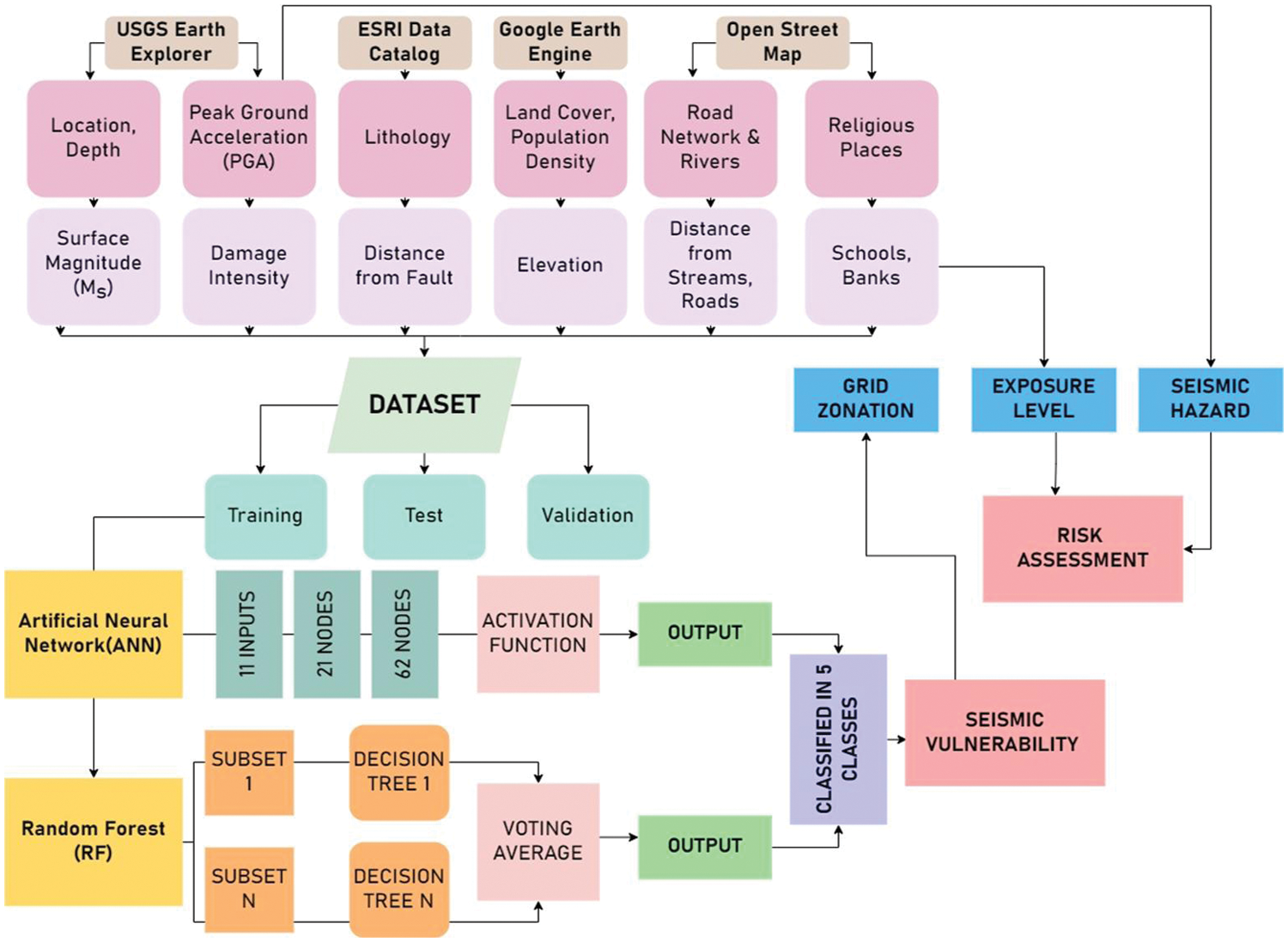
Figure 2: Workflow diagram

4  Data Used

USGS Earthquake Hazards Program monitors, reports, and research earthquakes and hazards. The USGS Earthquake Hazards Program of the U.S. Geological Survey (USGS) is part of the National Earthquake Hazards Reduction Program (NEHRP) led by the National Institute of Standards and Technology (NIST). Under this program, a database with the earthquake events has been curated that contains the location information, depth value, and magnitude value of each earthquake event that has occurred globally. The dataset has been utilized to extract natural earthquake events, not those caused by nuclear activities. The other variable values for the event points were extracted per the sources in the Table 1.

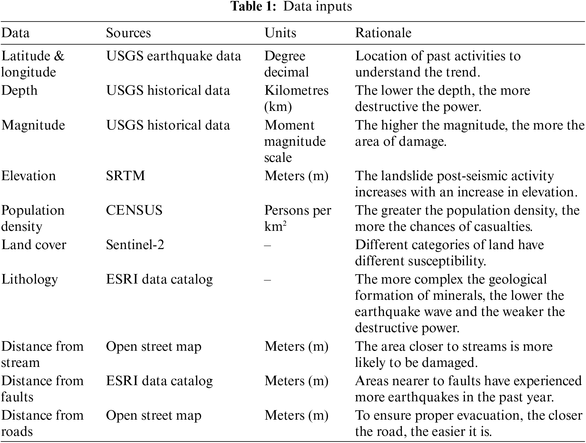
4.1 Satellite-Based and Other Products

This table presents key variables for seismic vulnerability modelling, including latitude, depth, magnitude, elevation, population density, land cover, lithology, distance from streams, faults, and roads. Each variable is sourced from specific datasets and measured in relevant units, aiding in understanding seismic trends and potential impact. The rationale behind each variable highlight factors such as geological formations, population density, and proximity to natural features affecting vulnerability assessments.

The training and testing dataset had records from the years 1900-01-01 to 2020-12-31.

4.2 In-Situ Calculations

The study used the magnitude values of the past earthquakes between 1900–2022, which were collected from the USGS Earthquake Data Catalog. It associated those different magnitude values (regional, moment, body, etc.) to surface magnitude value using the following formulae:

Ms=mb−2.74/0.46(1)

Ms=Mw−2.07/0.67(2)

where Ms is the surface magnitude, Mw is the Moment Magnitude, and mb is the body magnitude. A magnitude based on the amplitude of Rayleigh surface waves measured at a period near 20 s. Ms is primarily valuable for large (>6) shallow events, providing secondary confirmation on their size [17].

After gathering the surface magnitude value, the peak ground acceleration value for each earthquake incident was calculated using Donovan’s Formula:

PGA =1080e0.5Ms(R+25)−1.32(3)

where Ms is the surface magnitude, R = Distance from the hypocentre to the event’s site (in Kilometers), and peak ground acceleration (PGA) equals the maximum ground acceleration during earthquake shaking at a location.

PGA is a measure of how much ground shakes at a particular location during an earthquake event. It is calculated by looking at the highest acceleration record on an accelerogram device [18]. To understand the severity of an earthquake event, damage intensity values are considered, which helps in correlating the damages caused by an event with the magnitude.

Imm=2.20log⁡(PGA)+1.00 [for Ms values 3.5 to 5](4)

Imm=3.66log⁡(PGA)−1.66 [for Ms values 5+](5)

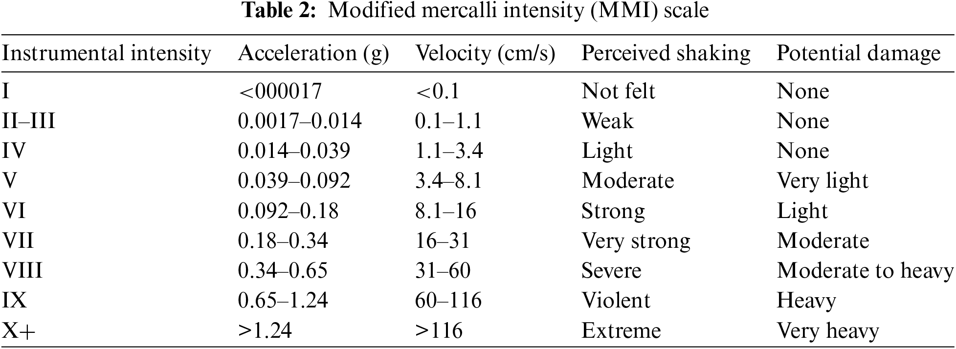
Each damage intensity value can be correlated to the Modified Mercalli Intensity values. Earthquakes cause different effects on the earth’s surface, known as the earthquake’s intensity. A scale has been developed to measure this intensity by considering the different observations of people who have experienced that event. This scale is called the Modified Mercalli Intensity scale and helps everyone understand the potential damage caused by the event [12].

The Modified Mercalli Intensity (MMI) scale is a subjective measurement scale used to assess the intensity of shaking experienced during an earthquake at a specific location. Unlike magnitude, which measures the energy released by an earthquake at its source, intensity describes the effects of the earthquake as perceived by people and the damage caused to structures and the environment [19].

The MMI scale is divided into 12 increasing levels, ranging from I (Not felt) to XII (Destruction). Each level corresponds to specific descriptions of shaking effects and associated damage. The descriptions are qualitative and based on observations of the earthquake’s impact on people, buildings, and the environment. The scale has been described in Table 2.

5  Exploratory Data Analysis (EDA)

EDA is the first step in any modelling study. With the help of EDA, the relationship between various factors is established, and data patterns are also analyzed. It gives us a basic understanding of how and which factor affects the predictor variable the most [20].

To initiate this study, we examined historical earthquake incident data from the past 100 years. This data consists of information regarding the location, magnitude, depth, time, and date of each incident. This examination aimed to understand the necessity of conducting this study. The results have been displayed in Figs. 3 and 4.

Figure 3: Number of earthquakes from 1904–2022

Figure 4: Graph for earthquakes above magnitude 7 (1904–2022)

The earthquake incidents were categorized by years, and their trends were studied, including the occurrences of earthquakes above magnitude 7. As depicted in the graphs above, there has been a substantial increase in the number of earthquakes between the years 1902 and 2022. Additionally, during the period from 2004 to 2013, the number of earthquakes with a magnitude above 7 reached its peak.

We are exploring the influence of various parameters before the architecture leads to a better understanding. While directly influencing the desired target parameter, the inputs do not account for the interaction between them.

In this study, the damage intensity values for each of the earthquake events above magnitude 3.5 were calculated between the years 1900 and 2022; using the USGS earthquake explorer data, the location (latitude, longitude), magnitude, and depth (distance from hypocentre, in km) was extracted. Other datasets like land cover, population density, elevation, distance from roads, significant rivers, distance from fault lines, and lithology type information were compiled from the abovementioned sources. All these data points were segregated into a 70:30 ratio for training (19040 records) & testing data (8160 records) and another validation dataset (another 786 records) with a temporal gap of 6 months before the building of models.

A correlation matrix (Fig. 5) was generated to understand the influence of the variables on each other by displaying the correlation coefficients for different variables. The correlation matrix depicted in Fig. 5 describes the potential level of influence between different parameters on a normalized scale. The image depicts the degree of influence between all the possible pairs of values used in this study.

Figure 5: Correlation matrix

The above correlation matrix shows that “distance from the fault line” negatively influences Z. This understanding is associated with higher elevations, like the Himalayan range, which tends to have fewer faults. Similarly, depth is inversely correlated to damage intensity at an extreme level. It can be confirmed that the more profound the epicentre, the shockwaves become before it touches the surface.

6  Model Development

6.1 Artificial Neural Network (ANN)

Artificial neural networks (ANNs) are biologically inspired computational networks [21].

Artificial neural networks are computer programs that simulate how the human brain and nervous system process information. These networks comprise individual processing units called neurons connected through weighted connections known as synaptic weights. The neurons process information received from other neurons to generate an output signal, which is achieved using an activation function. Neural networks come in two main types: feed-forward and feed-back.

They must be trained using an algorithm to make neural networks effective in their respective tasks. One popular algorithm is the Rectified Linear Unit (ReLu) activation function. ReLu is a piecewise linear function that outputs the input directly if it is positive and zero if it is negative. This activation function is beneficial when dealing with nonlinear functions and is easily trained with multilayer Perceptron and convolutional neural networks.

The gradient descent algorithm is another important aspect of neural network training. It is an optimization algorithm used to solve machine-learning problems. This algorithm approaches the optimal solution of the objective function by obtaining the minimum loss function and related parameters. There are two types of gradient descent algorithms: batch gradient descent and stochastic gradient descent. Batch gradient descent calculates gradients for the whole dataset, which can be time-consuming for large datasets. On the other hand, stochastic gradient descent performs one update at a time, which makes it much faster. However, it has a higher variance that causes the objective function to fluctuate heavily.

The present study applies a Stochastic Gradient Descent transfer function with ReLu activation for the estimation of the seismic vulnerability of India. The architecture has been depicted in Fig. 6.

Figure 6: ANN architecture

Eleven inputs (mentioned in Table 1) have been used in the model. Over multiple iterations, 16 combinations of input hyperparameters were fine-tuned to provide the optimized parameterized model. The number of hidden layers was kept as two as it performed better than the multi-layer perceptron model. The study adapts the standard conditions by Heaton, which follows the 2n-1 rule for the first hidden layer when selecting the number of nodes within each hidden layer, where n is the number of inputs and the 3n-1 rule for the second layer, making the first layer have 21 nodes and second layer have 62 nodes.

A two-layered artificial neural network was utilized for this study. The created datasets were segregated into a 70:30 ratio for training (19040 records) & testing data (8160 records). The model was trained and fine-tuned to optimize the results. The performance of the same can be seen in Figs. 7–9.

Figure 7: Hyperparameter curve for hidden layers

Figure 8: Hyperparameter curve for batch size

Figure 9: Hyperparameter curve for learning rate

The number of hidden layers in a neural network is decided, keeping the complexity of datasets in mind. For this study, it was noticed that increasing the hidden layers beyond 2 saturates the model’s accuracy, thus resulting in overfitting of the model.

The model training started with taking a batch size of 64 and checking the accuracy against the same. Simultaneously, the batch size was decreased to 16; and it was observed that the accuracy achieved was the best in this case. Keeping a batch size of 16 meant that the entire training data would pass through the model in batches of 16 observations at a point while training the model.

The hyperparameter controls the rate of learning or speed at which the model learns. It regulates the number of allocated errors with which the model’s weights are updated. The learning rate value is in the range of 0.0–1.0. This study’s accuracy value started saturating upon increasing the learning rate value beyond 0.1.

6.2 Random Forest (RF)

A random forest is a type of classifier that comprises a set of tree-structured classifiers {h(x, Θk), k = 1,...}. Each tree in the random forest casts a unit vote for the most commonly occurring class for the given input x. Moreover, the {Θk} represents independently and identically distributed random vectors [22].

Random Forest is a computer program that helps classify or make predictions based on data. It is commonly used in many applications such as predicting whether a customer will buy a product or identifying whether an email is spam or not. It works by using many small decision trees together to make a final decision, rather than relying on just one tree. The algorithm creates different training subsets from the sample training data with replacement, meaning that it can use the same data points more than once, making it more accurate. These subsets are selected randomly from the dataset and are called bootstrap samples. Therefore, each decision tree or model is produced using samples from the original data, with replacement, in a process called Bootstrapping. Each model is trained independently, generating individual results. The outcome is then formed by calculating the average output of all the decision trees. This step is called Aggregating. The design has been exemplified in Fig. 10.

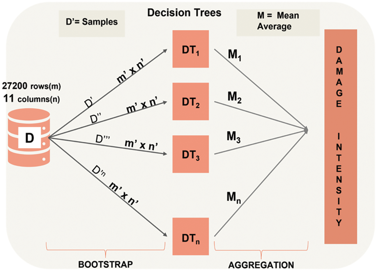
Figure 10: RF architecture

In this study, specific model parameters called hyperparameters are fine-tuned to improve the model’s performance. Random forest functions on the combination of multiple trees of varied degrees and levels. Each one is responsible for driving the model in an optimized form. The parameter “n_estimators” defines the number of trees within the algorithm based on the model tuning. Typically, increasing the number of trees in the random forest model leads to more generalized results. However, this also increases the time complexity of the model. The model’s performance increases with the number of trees but levels off after a certain point. The “max_depth” parameter is crucial, as it determines the longest path between the root and leaf nodes in each decision tree. Setting a large max_depth may result in overfitting. The “max_features” parameter determines the maximum number of input variables provided to each tree. The default value, which is the square root of the number of features in the dataset, is usually a good choice to consider.

A random forest was used to build several iterations of an RF model. Like ANN, the datasets created were randomly segregated into a 70:30 training and testing data ratio. The process of optimizing the model involves adjusting certain parameters to improve its accuracy. These parameters include “n_estimators,” which refers to the number of decision trees generated, “max_depth,” which is the longest distance between the root node and the leaf node, and “max_features,” which is the number of variables randomly selected as candidates at each node. The parameters were adjusted over several iterations of the model to assess how overall accuracy was affected by each. The overall performance of the architecture is depicted in Figs. 11–13.

Figure 11: Validation curve for max_depth

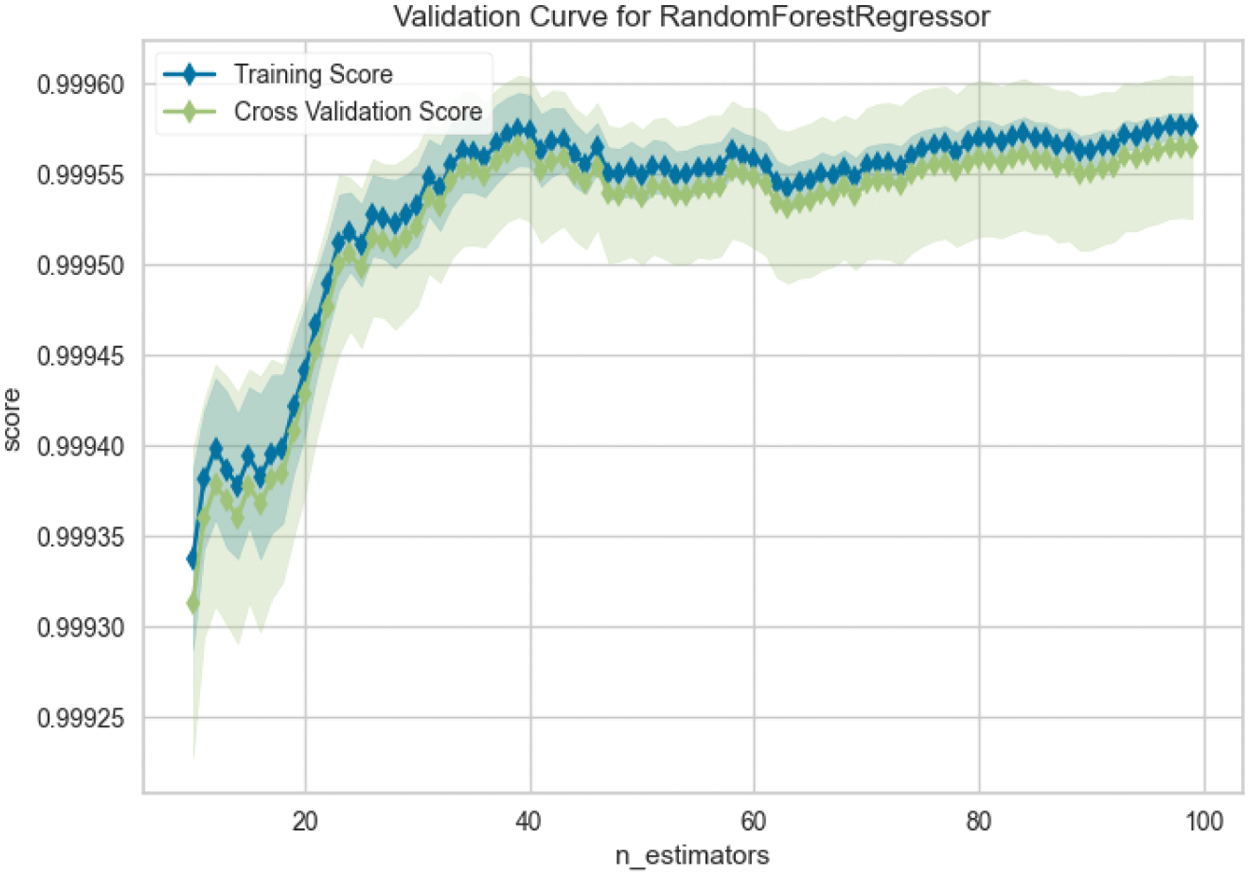
Figure 12: Validation curve for n_estimators

Figure 13: Validation curve for max_feature

It is essential to remember that max_depth is not the same thing as the depth of a decision tree. max_depth is a way to pre-prune a decision tree. This study observed that the model is achieving a threshold after max_depth 4.

A higher number of decision trees gives better results but slows the processing. The model attained maximum accuracy at 40 n_estimators (number of decision trees).

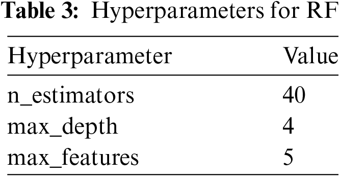
The max_features, if not specified, considers all the parameters. There are 11 input parameters, and the model attains maximum accuracy by using any random 5 of them. After this, it is sustained. Like ANN, the input and temporal periods are the same for the input dataset. This provides a better comparative capacity between the models. Within RF, the following fine-tuned parameterized values were identified for the final model. The following fine-tuned parameters are described in Table 3.

6.3 Sensitivity Analysis

Sensitivity analysis is the label used for a collection of methods for evaluating how sensitive model output is to changes in parameter values [23]. Sensitivity analysis identifies which input variables are essential in contributing to the prediction of the output variable. It quantifies how the changes in the input parameters’ values alter the outcome variable’s value [24].

The one-dimensional sensitivity focuses on varying one parameter while keeping the remaining constant. This can provide an understanding of the level of influence between the parameter and the output scale. For both the models, the mean values of input parameters were taken; for instance, in the case of depth, the mean value is 54.8 km, and the deviation of this value with 50% on either side of the mean value, i.e., plus and minus 25 kms and the result shows that it shifted damage intensity from −1.42 to 1.48. The parameters like streams, roads & population showed minimal sensitivity toward the damage intensity. This is known as one-way sensitivity analysis since only one parameter is changed simultaneously. The analysis was repeated on different parameters at various times, and the values have been depicted in Fig. 14.

Figure 14: Sensitivity analysis for (a) ANN, (b) RF

7  Results

The dataset was divided into training and testing subsets in a ratio of 70:30. Scatter plots were generated to evaluate the performance and accuracy of both the Random Forest model and the Artificial Neural Network model in terms of the Coefficient of Correlation (R), Mean Absolute Error (MAE), and Percentage Root Mean Square Error (PRMSE).

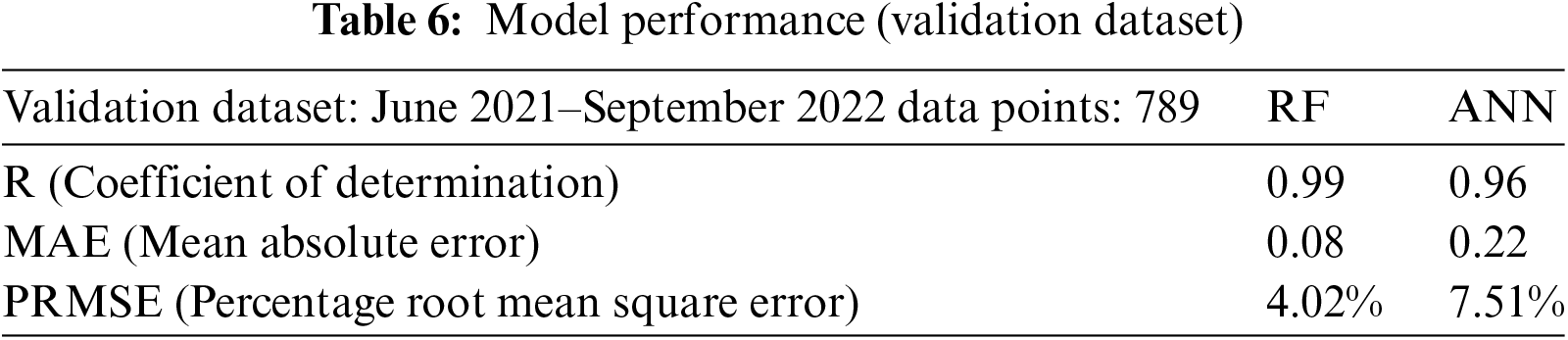
The training stage performance of both the models has been depicted in Fig. 15 and performance in Table 4; Test phase performance in depicted in Fig. 16 and Table 5, and validation is depicted in Fig. 17 and Table 6.

Figure 15: Training data scatter plot for (a) RF, (b) ANN

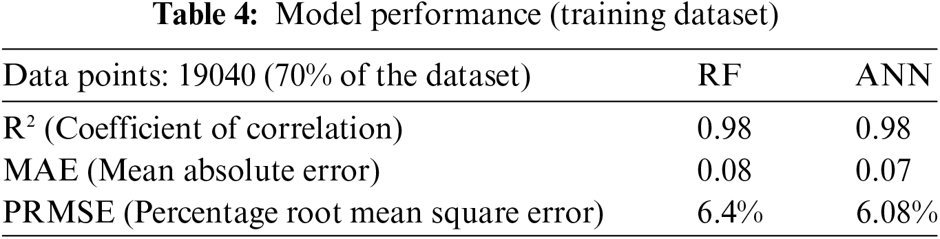
Figure 16: Test data scatter plot for (a) RF, (b) ANN

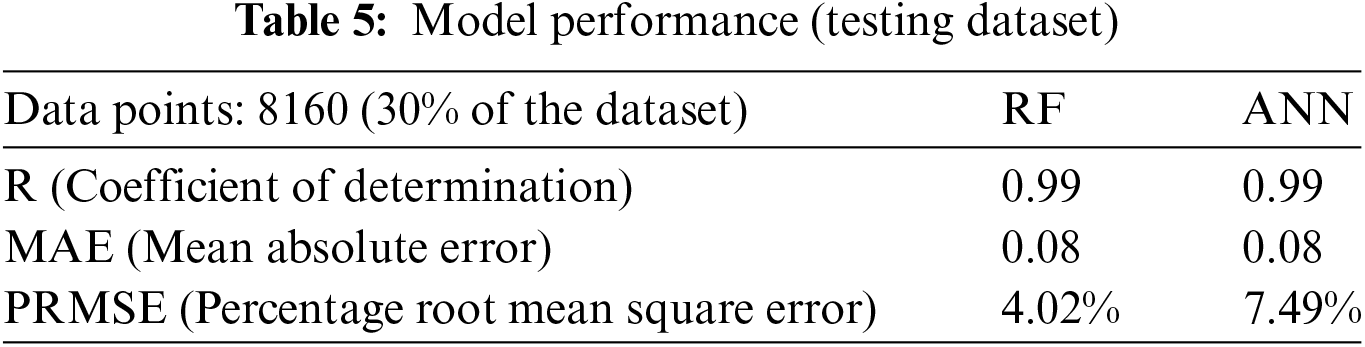
Figure 17: Validation data scatter plot for (a) RF, (b) ANN

The scatter plots for training data subsets of both models are providing a good accuracy and perform exceptionally well in predicting damage intensity values for earthquake events based on numerous factors, highlighting the effectiveness of the proposed approach in seismic vulnerability modelling.

From the scatter plots, the values obtained from the model are close to the actual values, along with some outlier values. Comparable results were seen upon testing the model with the remaining 8160 points of the datasets.

Lastly, to rule out any temporal dependencies of the model on the dataset, a new dataset with six months of the temporal gap was run through the model. The training and testing datasets had events until December 2020, and the new dataset (Validation Dataset) with 789 data points consisted of events from June 2021 until September 2022. For the validation dataset as well, it can be observed from the scatter plot and the metrics results that the model has performed exceptionally well.

7.1 Temporal Trend Analysis

The models performed closely; although the ANN model captured the peaks and dips of the damage intensity values, Random Forest performance was better in accuracy as it provided the average of the damage intensity values generated through each decision tree. Furthermore, a temporal analysis of the test dataset was plotted in Fig. 18 to depict the trend comparison between the actual and model values.

Figure 18: Validation curves

Specifically, the ANN model excelled in closely capturing the peaks and dips of the data values, providing a more nuanced geospatial representation, as depicted in the accompanying graphs and maps. Conversely, the Random Forest model, while generating output values closer to the actual data, displayed limitations in capturing extreme values. This distinction arises from the inherent nature of the Random Forest model, which operates as a bagging ensemble model, averaging the output values from multiple decision trees. As a result, the ANN model offers a richer depiction of the data’s variability, particularly in its ability to closely mirror the fluctuations in the dataset.

7.2 Upscaling to Spatial Scale

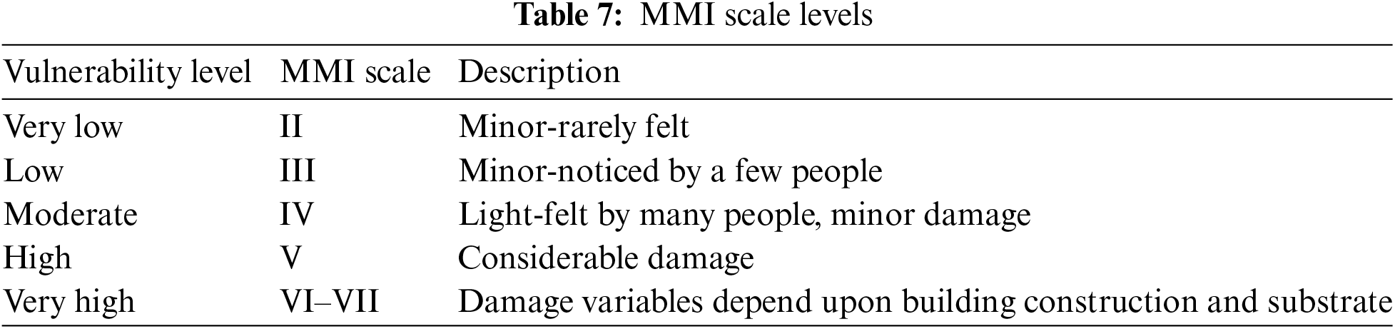
The resulting models were used to interpolate and upscale to a spatial scale of a 2 km grid. This approach will provide a good understanding of the spatial pattern and distribution over India. The classes were defined using the Modified Mercalli Intensity Scale as the reference to quantify the vulnerability, as mentioned in Table 7.

The maps below illustrate the varying vulnerability levels across India. Notably, while earthquake events are more frequent along the Northern belt, the vulnerability levels are higher along the Southern coast. This suggests that in the event of earthquakes of similar magnitude occurring along both the northern belt and the southern coast, the impact would be more devastating along the southern coast.

In the figure below, both model outputs are displayed spatially. Regions classified as high and extremely high vulnerability areas often experience lower earthquake frequencies compared to areas marked as shallow and low-risk zones. This implies that an earthquake of significant magnitude would pose a greater threat to regions in southern and central India. This heightened vulnerability can be attributed to the concentration of population and infrastructure in these areas, which lack resilience against seismic activities, thus amplifying potential damage.

The subsequent maps (Fig. 19) reveal the diverse vulnerability levels across India. Noteworthy is the fact that while areas with the highest frequency of earthquakes often fall within the low and extremely low vulnerability zones, regions with lower frequencies, such as Maharashtra, are categorized as high-vulnerability areas. This distinction is primarily due to factors such as population density and the lack of seismic considerations in infrastructure planning.

Figure 19: Seismic vulnerability map for India (Model outputs)

7.3 Case Study Example

A risk map for the entire India can be generated using the Seismic vulnerability map. For example, a risk map for Satara district, Maharashtra, was generated as the application area of this study. The location is shown in Fig. 20.

Figure 20: Satara district map

The Satara district of Maharashtra experienced an earthquake of 5.0 magnitude on 16 September 2008. It has an area of 10,480 km2 and a population of 3,003,741, of which 14.17% were urban (as of 2011). Although the magnitude was not much, the damage was alarming. 606 buildings were severely damaged in 110 villages, and another 573 buildings in 92 villages in Patan taluka also inflicted minor damage within 100 km of the epicentre. This engenders a need to be prepared if such an event happens again. For this purpose, a hazard map was generated from the Global Seismic Hazard map. The exposure map was created after overlaying maps of different areas like schools, banks, and other public spaces. Finally, a risk map was created. For Satara district to understand the potential losses in terms of lives, health, economy, and livelihood. The risk map was categorized into five risk levels, and the at-risk population was estimated. The risk map depicts that around 40% of the district falls under moderate to high-risk levels, with 44% of the population at risk. The following images (Figs. 21 and 22) show the potential levels of hazard, vulnerability and exposure for the region.

Figure 21: (a) A hazard map, (b) a vulnerability map, and (c) an exposure map for the Satara district of Maharashtra

Figure 22: Satara district risk level map

8  Discussion

In this study, both the Artificial Neural Network (ANN) and Random Forest (RF) models exhibited commendable performance. The accuracy of these models was notably similar; however, the Random Forest model demonstrated a slight advantage over the ANN model. Notably, the ANN model’s ability to closely capture the peaks and dips of the data values provided a richer geospatial representation, as evidenced by the graphs and maps. In contrast, the Random Forest model, while generating output values closer to the actual data, exhibited limitations in capturing extreme values. This is inherent like a Random Forest, as it operates as a bagging ensemble model, averaging the output values from multiple decision trees.

Comparing this study’s findings to previous research, which explored hybrid models based on Artificial Neural Networks for GIS-based seismic vulnerability mapping, similarities in model performance are apparent. It noted the effectiveness of hybrid models in providing detailed seismic vulnerability maps, a sentiment echoed in this study regarding the ANN model’s geospatial representation. Similarly, another research delved into machine learning techniques for urban-scale seismic vulnerability assessment, highlighting parallels with our use of ANN and RF models. Their work, focusing on building characteristics and soil types, mirrors our study’s approach to understanding seismic vulnerability through these models.

Moreover, the study on GIS-based rapid earthquake exposure and vulnerability mapping aligns with similar suggestions for future research directions. They emphasized the importance of finer-resolution datasets, a notion echoed in this study [3,4,25].

As this study has been done on a coarser resolution of 2 km × 2 km, moving forward, finer resolution datasets can provide more granular insights into the seismic vulnerability of specific areas. Moving forward, incorporating more parameters such as building materials and age-wise population, as suggested by other studies could enhance the holistic understanding of seismic vulnerability. Looking ahead, the exploration of alternative models such as Long Short Term Memory (LSTM) and Teaching Learning Based Optimization (TLBO), presents intriguing avenues for further investigation [21,26].

9  Conclusion

Earthquakes, with their potential for devastating impacts on lives, infrastructure, and economies, stand among the most unpredictable and hazardous natural events. This study has introduced a novel approach to seismic vulnerability modelling for India, leveraging the power of Machine Learning (ML) algorithms and Geographic Information Systems (GIS). The aim was to address the notable gaps in previous research by predicting damage intensity values for earthquake events based on a multitude of factors. These factors include location, depth, land cover, proximity to major roads, rivers, soil type, population density, and distance from fault lines.

Both the Artificial Neural Network (ANN) and Random Forest (RF) models demonstrated exceptional accuracy, exceeding 95% for both training and testing datasets. The ANN model highlighted a closer representation of the peaks and dips in data values, while the RF model excelled slightly in overall accuracy, providing an average of damage intensity values generated through decision trees. The models were not just confined to theoretical accuracy. They found practical application in the case study of the Satara district in Maharashtra, illuminating vulnerable buildings and enhancing seismic risk assessment at a local level. This case study exemplified how the models can estimate potential losses in terms of lives, health, economy, and livelihoods, offering invaluable insights for disaster management and urban planning decision-makers.

Moreover, this study extended beyond mere modelling; it aimed to provide actionable tools for risk reduction. By generating a zonation map categorizing regions into Very High, High, Moderate, Low, and Very Low vulnerability classes, a visual representation of exposure grids was created. This vulnerability index map aids in identifying regions requiring immediate risk reduction interventions and offers a comprehensive understanding of risk metrics associated with different areas. It can guide decision-makers in resource allocation and the implementation of targeted strategies to minimize the potential loss of human lives and financial damage from future earthquakes.

In summary, this study represents a significant stride in the field of seismic risk assessment, offering a robust framework that combines ML algorithms and GIS technology. By empowering decision-makers with precise insights into seismic vulnerability, this approach stands poised to enhance disaster preparedness, mitigation, and management strategies, fostering a more resilient future for communities in India vulnerable to seismic hazards.

Acknowledgement: We want to thank the Faculty of Technology, CEPT University, and CEPT University management for providing the infrastructure and support to call out this study.

Funding Statement: The authors received no specific funding for this study.

Author Contributions: Shalu did the data acquisition and data processing, developed the ANN model, conducted validation and analysis, and drafted the manuscript. Twinkle Acharya developed the Random forest model and edited the manuscript. Dhwanilnath Gharekhan guided and supervised the analysis and model development and drafted and edited the manuscript. Dipak R Samal guided and supervised the analysis and model development.

Availability of Data and Materials: The data will be made available on request by contacting the corresponding author, dhwanilnath@gmail.com.

Conflicts of Interest: The authors declare that they have no conflicts of interest to report regarding the present study.

References

1. Manishs IQ. Earthquakes in India types, map, zones, causes, impacts. 2022. Available from:https://www.studyiq.com/articles/earthquakes-in-india/ [Accessed 2022]. [Google Scholar]

2. Lee S, Panahi M, Pourghasemi HR, Shahabi H, Alizadeh M, Shirzadi A, et al. Sevucas: a novel gis-based machine learning software for seismic vulnerability assessment. Appl Sci. 2019 Aug 24;9(17):3495. [Google Scholar]

3. Yariyan P, Avand M, Soltani F, Ghorbanzadeh O, Blaschke T. Earthquake vulnerability mapping using different hybrid models. Symmetry. 2020 Mar 4;12(3):405. [Google Scholar]

4. de Los Santos MJ, Principe JA. Gis-based rapid earthquake exposure and vulnerability mapping using lidar dem and machine learning algorithms: case of porac, pampanga. Int Arch Photogramm, Remote Sens Spatial Inf Sci. 2021 Nov 18;46:125–32. [Google Scholar]

5. Burton C, Cutter SL. Levee failures and social vulnerability in the Sacramento-San Joaquin Delta area, California. Nat Hazard Rev. 2008 Aug;9(3):136–49. [Google Scholar]

6. Wang Z. Seismic hazard vs. seismic risk. Seismol Res Lett. 2009 Sep 1;80(5):673–4. [Google Scholar]

7. Wang Z. Seismic hazard assessment: issues and alternatives. Pure Appl Geophys. 2011 Jan;168:11–25. [Google Scholar]

8. Sinha R, Aditya KS, Gupta A. GIS-based urban seismic risk assessment using RISK. IITB. ISET J Earthquake Tech. 2008;45:41–63. [Google Scholar]

9. Stein S, Geller RJ, Liu M. Why earthquake hazard maps often fail and what to do about it. Tectonophys. 2012 Aug 24;562:1–25. [Google Scholar]

10. van Westen CJ. Remote sensing and GIS for natural hazards assessment and disaster risk management. Treatise Geomorphol. 2013 Mar;3(15):259–98. [Google Scholar]

11. Nhu VH, Shirzadi A, Shahabi H, Singh SK, Al-Ansari N, Clague JJ, et al. Shallow landslide susceptibility mapping: a comparison between logistic model tree, logistic regression, naïve bayes tree, artificial neural network, and support vector machine algorithms. Int J Environ Res Public Health. 2020 Apr;17(8):2749. [Google Scholar] [PubMed]

12. Wald DJ, Quitoriano V, Heaton TH, Kanamori H. Relationships between peak ground acceleration, peak ground velocity, and modified Mercalli intensity in California. Earthq Spectra. 1999 Aug;15(3):557–64. [Google Scholar]

13. Bosher L, Chmutina K. Disaster risk reduction for the built environment. England: John Wiley & Sons; 2017 Jun 12. [Google Scholar]

14. Corominas J, van Westen C, Frattini P, Cascini L, Malet JP, Fotopoulou S, et al. Recommendations for the quantitative analysis of landslide risk. Bull Eng Geol Environ. 2014 May;73:209–63. [Google Scholar]

15. Verma M, Bansal BK. Seismic hazard assessment and mitigation in India: an overview. Int J Earth Sci. 2013 Jul;102:1203–18. doi:10.1007/s00531-013-0882-8. [Google Scholar] [CrossRef]

16. Gupta ID. Delineation of probable seismic sources in India and neighbourhood by a comprehensive analysis of seismotectonic characteristics of the region. Soil Dyn Earthq Eng. 2006 Aug 1;26(8):766–90. doi:10.1016/j.soildyn.2005.12.007. [Google Scholar] [CrossRef]

17. Maradudin AA, Mills DL. The attenuation of Rayleigh surface waves by surface roughness. Annals Phys. 1976 Sep 10;100(1–2):262–309. [Google Scholar]

18. Puteri DM, Affandi AK, Sailah S, Hudayat N, Zawawi MK. Analysis of peak ground acceleration (PGA) using the probabilistic seismic hazard analysis (PSHA) method for Bengkulu earthquake of 1900–2017 period. J Physics: Conf Series. 2019 Jul 1;1282(1):12054. [Google Scholar]

19. Serva L, Vittori E, Comerci V, Esposito E, Guerrieri L, Michetti AM, et al. Earthquake hazard and the environmental seismic intensity (ESI) scale. Pure Appl Geophys. 2016 May;173:1479–515. doi:10.1007/s00024-015-1177-8. [Google Scholar] [CrossRef]

20. Behrens JT. Principles and procedures of exploratory data analysis. Psychol Methods. 1997 Jun;2(2):131. doi:10.1037/1082-989X.2.2.131. [Google Scholar] [CrossRef]

21. Park YS, Lek S. Artificial neural networks: Multilayer perceptron for ecological modeling. In: Developments in environmental modelling, vol. 28. Elsevier; 2016 Jan 1. p. 123–40. [Google Scholar]

22. Kuznetsova N, Westenberg M, Buchin K, Dinkla K, van den Elzen SJ. Random forest visualization. Eindhoven, Netherlands: Eindhoven University of Technology; 2014 Aug. [Google Scholar]

23. Franceschini S, Tancioni L, Lorenzoni M, Mattei F, Scardi M. An ecologically constrprocedure for sensitivity analysis of artificial neural networks and other empirical models. PLoS One. 2019 Jan 30;14(1):e0211445. doi:10.1371/journal.pone.0211445. [Google Scholar] [PubMed] [CrossRef]

24. Gevrey M, Dimopoulos I, Lek S. Two-way interaction of input variables in the sensitivity analysis of neural network models. Ecol Model. 2006 May 15;195(1–2):43–50. doi:10.1016/j.ecolmodel.2005.11.008. [Google Scholar] [CrossRef]

25. Ferranti G, Greco A, Pluchino A, Rapisarda A, Scibilia A. Seismic vulnerability assessment at an Urban scale by means of machine learning techniques. Buildings. 2024 Feb;14(2):309. doi:10.3390/buildings14020309. [Google Scholar] [CrossRef]

26. Martins L, Silva V. Development of a fragility and vulnerability model for global seismic risk analyses. Bull Earthq Eng. 2021 Dec;19(15):6719–45. doi:10.1007/s10518-020-00885-1. [Google Scholar] [CrossRef]