An Intrusion Detection Method Based on a Universal Gravitation Clustering Algorithm

Abbreviations

1  Introduction

With the exponential growth of information technology and the widespread utilization of the Internet and cloud computing, the Internet has become an essential component of people’s daily lives and professional endeavors. However, although it offers numerous benefits, the Internet is also confronting more severe security challenges, among which network intrusion is a particularly threatening activity. Hackers employ various tactics to breach network security, steal confidential information, disrupt system operations [1–3], and even compromise national security. Considering these threats, intrusion detection has emerged as a critical task in network security. Traditional intrusion detection techniques primarily relies on rules and feature engineering [4–8]. These methods can be effective in certain scenarios, while exhibiting certain limitations. First, the development of rules and feature engineering necessitates the expertise and knowledge of specific specialists, which can restrict their ability to adapt to the continuous evolution of network intrusion. Second, these methods may result in an excessive number of false alarms, thereby compromising detection efficiency. Therefore, researchers have explored more sophisticated and adaptable intrusion detection methods.

Clustering is a data analysis and machine learning method that involves grouping or dividing objects in a dataset into subsets with similar characteristics or attributes, known as “clusters” [9]. The primary objective of clustering is to separate data into meaningful groups without relying on pre-existing labels or category information to uncover the underlying patterns or structures in the data. The primary purpose of the clustering algorithm is to quantify the similarity or dissimilarity between data objects using specific measurements and subsequently group similar objects into the same cluster to minimize intra-cluster differences and maximize inter-cluster differences. Cluster analysis is a highly versatile, multivariable statistical method that exhibits a wealth of information and diverse applications. Commonly employed techniques include dynamic clustering [10], ordered sample clustering, fuzzy clustering [11], clustering forecasting methods, and graph clustering methods [12,13]. Moreover, clustering plays a crucial role in the detection of anomalous behaviors.

The problem of detecting abnormal behavior in network users has been the subject of numerous studies conducted by various scholars. Reference [14] utilized the built-in typical classification algorithm of the Weka machine-learning software tool to conduct classification research on intrusion detection datasets for cloud computing. Specifically, the naive Bayes algorithm was implemented to classify the abnormal behavior of intranet users using software engineering methods. The experimental results, which aimed to classify malicious and normal behaviors, indicated that the naive Bayes algorithm implemented in that study exhibited high classification accuracy and was effective in classifying, analyzing, and mining intranet user behaviors in cloud computing intrusion detection datasets. Regarding the limitations of simple threshold detection, reference [15] proposed a method for detecting anomalies in smart substation process layer network traffic using differential sequence variance. Reference [16] extracted frequency domain features from smart substation flow data and combined them with time-domain features to create a time-frequency domain hybrid feature set, which was used to identify abnormal flow. Machine learning techniques were employed in the literature [17–19] to detect abnormal flow data in industrial power controls. Reference [20] introduced an outlier detection method based on Gaussian mixture clustering, utilizing time-series features of power industrial control system data. Reference [21] formulated rules based on the IEC (International Electrotechnical Commission) 61850 protocol and performed intrusion detection on the data collection and monitoring systems of smart substations applying the devised rules. In addition, references [22,23] implemented outlier detection on IEC 60870-5-104 protocol messages according to the rules. Furthermore, reference [24] proposed a method that utilized blacklist and whitelist of business logic and similarity matching to identify attack messages.

The problem of detecting abnormal user behavior can be viewed as a clustering problem in which normal behavior data are clustered together and abnormal behavior data are clustered separately. The objective of this outlier analysis technique is to categorize an object being tested into several classes or clusters [25]. Recently, advancements in machine learning and data mining technology have created new prospects for intrusion detection [26]. As a valuable unsupervised learning technique, the clustering algorithm has been extensively applied in the domain of intrusion detection. Owing to its capacity to detect potential patterns and anomalies in data, it offers innovative insights for intrusion detection. However, traditional clustering algorithms also exhibit certain shortcomings in the context of intrusion detection, such as their inability to effectively adapt to high-dimensional data and their limited capacity to handle unbalanced datasets [27–30].

This study provides a concise overview of the primary classifications, advantages, and disadvantages of existing IDS, as shown in Table 1.

This study introduced a novel intrusion detection method based on a universal gravitation clustering algorithm to overcome the limitations of conventional approaches. The design principles, essential procedures, and experimental results of the method were elucidated, followed by a comparison with existing methods to verify its performance and efficacy. The integration of advanced clustering algorithms was expected to provide a fresh perspective and approach to intrusion detection in the realm of network security, ultimately enhancing the accuracy and efficiency of such detection and strengthening the network security.

The primary achievements of this study were as follows: (1) The development of a novel clustering algorithm, termed the “universal gravitation clustering algorithm”, which contrasted with traditional clustering techniques, such as K-means and hierarchical clustering. This algorithm utilized a gravitational model to describe the connections between objects to distinguish and cluster the aberrant behaviors of network users. Moreover, it seeks to identify potential intrusion behaviors in network intrusion detection. By incorporating dissimilarity and similarity analyses, abnormal behavior distinct from normal behavior was detected more accurately. (2) The algorithm adopted a dynamic cluster construction approach, beginning with an empty cluster and subsequently assigning new objects. This adaptable nature enabled the algorithm to respond to changes in network traffic and user behavior. (3) It utilized a specified correlation range threshold and difference definition to calculate the disparity between the new object and each existing cluster and selected the cluster with the smallest dissimilarity. This approach enhanced the precision of object assignment to their respective clusters. Furthermore, the integration of this innovative clustering algorithm may improve the efficiency of intrusion detection, making it more suitable for the realm of network security, and enabling it to detect and identify network intrusion behaviors more effectively, thereby enhancing network security.

2  Related Studies

2.1 Related Concepts

The inherent properties of user behavior exhibit inconsistencies in statistical characteristics across various user behaviors. The clustering-based user behavior outlier analysis method employs partially labeled training samples, leveraging their inherent differences to adapt to the disparities between normal and abnormal behaviors. Subsequently, collaborative methods were applied to analyze and identify abnormal user behaviors. This study began by proposing the following definitions to develop an accurate outlier analysis model:

Definition 1 (User behavioral features): The features of user behavior can reflect the differences between normal behavior and abnormal behavior, which may include user inquiries, running routes, and commencement and conclusion of methodological operations. These distinctions can be depicted using the cluster Cindex={C1,C2,⋯,Ci,⋯,Cn}.

Definition 2 (Training sample): The training sample represents the training samples of the data as shown in Eq. (1), where xij represents the behavioral characteristics of user i, with si∈{1,−1,0}, where 1 represents normal behavior, −1 represents abnormal behavior, and 0 represents unknown type of behavior.

D=(x11x12…x1ns1x21x22…x2ns2⋮⋮⋮⋮xm1xm2…xmnsm)(1)

Definition 3 (Neighborhood): If S(i)={j|d(i,j)≤R}, then node j is a neighbor of node i. If {i∈S(j)}∩{j∈S(i)} is not empty, then nodes i and j are neighbors, and their common neighbors form the neighborhood set Ωij, with Ωij={(S(i)∩S(j))}, as shown in Fig. 1. The slashed part in Fig. 1 is the neighborhood of nodes i and j.

Figure 1: Neighborhood of nodes i and j

2.2 User Abnormal Behavior Clustering Representation Model

Assume that the dataset D has m attributes, including mC categorical attributes and mN numeric attributes, with m=mC+mN. We might also assume that the categorical attributes are located before the numeric attributes and use Di to represent the set of ith attribute values. Due to the unique correspondence between an object and its identifier (which can be considered a record number), it is sometimes the case that an object is identified by its identifier.

Definition 4: Given clusters C and a∈Di, the frequency of a in C with respect to Di is defined as the number of times that a is included in the projection of C on Di.

FreqC|Di(a)=|{object | object∈C, object Di=a}|(2)

Definition 5: Given cluster C, the CSI of C is defined as:

CSI={n, Summary}(3)

where n=|C| or C, i.e., n is the size of C, and Summary consists of two parts: Frequency information of different values in categorical attributes and centroid of numerical attributes, namely.

Summary={⟨Stati, Cen ⟩|Stati={(a, Freq C∣Di(a))|a∈Di}1≤i≤mCCen=(cmC+1,cmC+2,⋯,cmC+mN)}(4)

2.3 Difference Analysis

The data spaces of two adjacent nodes can be divided into two subspaces: Categorical attributes and numerical attributes. The distance between the data in the entire space was then categorized into the distance between these two subspaces. In a linear space, the Minkowski distance can be expanded to yield the following definition:

Definition 6: Given clusters C of D, C1 and C2, objects of p=[p1,p2,⋯,pm] and q=[q1,q2,⋯,qm], y>0, z>0.

(1) The degree of difference (or distance) dif(pi,qi) between objects p and q on attribute i is defined as:

For categorical or binary attributes,

dif(pi,qi)={1,pi≠qi0,pi=qi

or dif(pi,qi)=1−{0,pi≠qi1,pi=qi

For continuous numerical attributes or ordinal attributes,

dif(pi,qi)=|pi−qi|(5)

(2) The distance d(p,q) between objects p and q is expressed as:

d(p,q)=dC+dNm(6)

The distance dC of the classification attribute part is defined as the sum of the differences in each classification attribute:

dC=∑i=1mCdif(pi,qi)(7)

The distance dN of the numerical attribute part is the Minkowski distance:

dN=(∑i=mC+1mC+mN|pi−qi|z)1z(8)

(3) The distance between object p and cluster C, d(p,C) is defined as the distance between p and the summary of cluster C, which consists of two parts.

d(p,C)=dC+dNm(9)

where the distance dC of the classification attribute part is defined as:

dC=(∑i=1mCdif(pi,C|Di)y)1y(10)

where dif(pi,C|Di) is the average distance between p and each object in C on attribute Di, that is:

dif(pi,C|Di)=1−FreqC|Di(pi)|C|(11)

The distance dN of the numerical attribute part is defined as the Minkowski distance between p and the centroid of C:

dN=(∑i=mC+1mC+mM|pi−ci|z)1z(12)

(4) The distance d(C1,C2) between clusters C1 and C2 is defined as the distance between two summaries and consists of two parts.

d(C1,C2)=dC+dNm(13)

where the distance dC of the classification attribute part is defined as:

dC=(∑i=1mCdif(C1|Di,C2|Di)y)1y(14)

where dif(C1|Di,C2|Di) is the average distance in attribute Di between any object p in C1 and any object q in C2, that is:

dif(C1|Di,C2|Di)=1−1|C1|⋅|C2|∑p∈C1Freq C1|Di(pi)⋅ Freq C2|Di(pi)=1−1|C1|⋅|C2|∑q∈C2 Freq C1|Di(qi)⋅ Freq C2|Di(qi)(15)

The distance dN of the numerical attribute part is defined as the Minkowski distance between the centroids of C1 and C2.

dN=(|ci(1)−ci(2)|z)1z(16)

Definition 7: Given clusters C of D, C1 and C2, objects p=[p1,p2,⋯,pm] and q=[q1,q2,⋯,qm], and x>0.

(1) The degree of difference (or distance) dif(pi,qi) between objects p and q on attribute i is defined as:

For categorical attributes or binary attributes,

dif(pi,qi)={1,pi≠qi0,pi=qi(17)

For continuous numerical attributes or ordinal attributes,

dif(pi,qi)=|pi−qi|(18)

(2) The degree of difference (or distance) d(p,q) between two objects p and q is defined as the power average of the degree of difference on each attribute, that is:

d(p,q)=(∑i=1mdif(pi,qi)xm)1x(19)

(3) The distance between object p and cluster C, d(p,C), is defined as the distance between p and the summary of cluster C:

d(p,C)=(∑i=1mdif(pi,Ci)xm)1x(20)

where dif(pi,Ci) is the distance between p and C on attribute Di.

For categorical attribute Di, its value is defined as the arithmetic mean of the distance between p and each object in C on attribute Di, that is:

dif(pi,Ci)=1− Freq C|Di(pi)|C|(21)

For a numeric attribute Di, its value is defined as:

dif(pi,Ci)=|pi−ci|(22)

(4) The distance d(C1,C2) between clusters C1 and C2 is defined as the distance between two abstracts:

d(C1,C2)=(∑i=1mdif(Ci(1),Ci(2))xm)1x(23)

where dif(Ci(1),Ci(2)) is the distance between C1 and C2 on attribute Di.

For a categorical attribute Di, the value is defined as:

dif(Ci(1),Ci(2))=1−1|C1|⋅|C2|∑pi∈C1 Freq C1|Di(pi)⋅ Freq C2|Di(pi)=1−1|C1|⋅|C2|∑qi∈C2FreqC1|Di(qi)⋅FreqC2|Di(qi)(24)

For a numerical attribute Di, the value is defined as:

dif(Ci(1),Ci(2))=|ci(1)−ci(2)|(25)

Definition 8: Given clusters C of D, C1 and C2, objects p=[p1,p2,…,pm] and q=[q1,q2,⋯,qm].

(1) The distance d(C1,C2) between clusters C1 and C2 is defined as:

d(C1,C2)=∑i=1mdif(Ci(1),Ci(2))m(26)

where dif(Ci(1),Ci(2)) is the difference in attribute Di between C1 and C2.

For a categorical attribute Di, the value is defined as:

dif(Ci(1),Ci(2))=∑a∈(C1∪C2)|Di Freq C1|Di(a)+FreqCC2|Di(a)|C1|+|C2|⋅|Freq C1|Di(a)|C1|−Freq C2|Di(a)|C2||Freq C1|Di(a)|C1|+Freq C2|Di(a)|C2|(27)

Frequency sets of different values are used to represent classification attributes.

If a∉C|Di, then Freq C|Di(a)=0.

For a numerical attribute Di, the value is defined as:

dif(Ci(1),Ci(2))={0,ci(1)=0 and ci(2)=0|ci(1)−ci(2)||ci(1)|+|ci(2)|,ci(1)≠0 or ci(2)≠0(28)

where ci(1) and ci(2) correspond to the centroids of C1 and C2 on attribute Di.

In particular, when a cluster contains only one object, two distinct definitions are obtained.

(2) The distance d(p,C) between object p and cluster C is defined as:

d(p,C)=∑i=1mdif(pi,Ci)m(29)

where dif(pi,ci) is the difference between p and C in attribute Di.

For a categorical attribute Di, the value is defined as:

dif(pi,Ci)=|C|+1+2⋅Freq C|Di(pi)|C|+1⋅|C|−Freq C|Di(pi)|C|+Freq C|Di(pi)(30)

For a numerical attribute Di, the value is defined as:

dif(pi,Ci)={0,pi=0 and ci=0|pi−ci||pi|+|ci|,pi≠0 or ci≠0(31)

where ci corresponds to the centroid of C on the attribute Di.

(3) The distance between objects p and q is defined as:

d(p,q)=∑i=1mdif(pi,qi)m(32)

where dif(pi,qi) represents the difference between p and q on the attribute Di.

For categorical attributes, the value of dif(pi,qi) is defined as:

dif(pi,qi)={0,pi=qi1,pi≠qi(33)

For continuous numerical attributes, the value is defined as:

dif(pi,qi)={0,pi=0 and qi=0|pi−qi||pi|+|qi|,pi≠0 or qi≠0(34)

Definition 8 is an extension of the Canberra distance.

Definition 9: Given clusters C of D, C1 and C2, objects p=[p1,p2,⋯,pm] and q=[q1,q2,⋯,qm],

(1) The distance d(C1,C2) between clusters C1 and C2 is defined as:

d(C1,C2)=(∑i=1mdif(Ci(1),Ci(2))xm)1x(x>0)(35)

where dif(Ci(1),Ci(2)) is the difference between C1 and C2 in attribute Di.

For a categorical attribute Di, the value is:

dif(Ci(1),Ci(2))=12∑pi∈(C1∪C2)|Di| Freq C1|Di(pi)|C1|− Freq C2|Di(pi)|C2||(36)

Categorical attributes are represented by frequency sets of different values. If a value does not appear, the frequency is zero.

For a numerical attribute Di, the value is defined as:

dif(Ci(1),Ci(2))=|ci(1)−ci(2)|(37)

Specifically, when a cluster contains only one object, two distinct definitions are obtained.

(2) The distance d(p,C) between object p and cluster C is defined as:

d(p,C)=(∑i=1mdif(pi,Ci)xm)1x(x>0)(38)

where dif(pi,Ci) is the difference between p and C in attribute Di.

For a categorical attribute Di, the value is:

dif(pi,Ci)=12(1−FreqC|Di(pi)|C|+∑qi∈C|Di,qi≠piFreqC|Di(qi)|C|)=1−Freq C|Di(pi)|C|(39)

For a numerical attribute Di, the value is defined as:

dif(pi,Ci)=|pi−ci|(40)

(3) The distance d(p,q) between objects p and q is defined as:

d(p,q)=(∑i=1mdif(pi,qi)xm)1x(x>0)(41)

where dif(pi,qi) represents the difference between p and q in attribute Di.

For categorical or binary attributes, the value is:

dif(pi,qi)={1,pi≠qi0,pi=qi=1−{0,pi≠qi1,pi=qi(42)

For continuous numerical or ordinal attributes, the value is:

dif(pi,qi)=|pi−qi|(43)

Note: In Definition 9, the relational expression ∑qi∈C|DiFreq C|Di(qi)=|C| is used. In actual application, numeric attributes need to be normalized within the range of [0,1].

It is evident that the distance given in Definition 9 satisfies several basic properties:

(1) d(C1,C2)=d(C2,C1)

(2) dif(Ci(1),Ci(2))≤1

For categorical attributes, the equal sign holds if and only if (C1|Di)∩(C2|Di)=∅.

(3) 0≤d(C1,C2)≤1

d(C1,C2)=0, if and only if the value and corresponding frequency of each classification attribute of the two classes are identical, and the centroid of each numerical attribute is constant, the two classes can be regarded as the same.

d(C1,C2)=1, if and only if the values of each categorical attribute of the two classes are different, and the centroid of each numerical attribute is zero for one class and one for the other class.

(4) If FreqC|Di(pi)≤FreqC|Di(qi), then dif(pi,Ci)≥dif(qi,Ci).

Especially, dif(pi,Ci)≥dif(pi∗,Ci), where pi∗ satisfies:

FreqC|Di(pi∗)=max{FreqC|Di(qi)|qi∈Ci}(44)

This property resembles the core theorem, on which the k-modes algorithm was proposed in [31].

To mitigate the impact of different measurement units on the outcomes, it is essential to standardize numerical attributes. As demonstrated in Definitions 6 to 9, the distance on each categorization attribute falls within the range of [0,1]. Adopting the average primarily serves to neutralize the impact of the attribute count on the distance value and confine the ultimate distance within [0,1], thereby facilitating comparison.

It is readily apparent that Definitions 6 and 7 are equivalent when the values of x, y, and z are all set to 1. This scenario is analogous to the extension of Manhattan distance. In this case, for categorical datasets with purely categorical attributes, the distance between two objects is a simple matching coefficient, as described in the literature, where x, y, and z all take the value of two. This aligns with the generalization of Euclidean distance. As distance is only utilized for comparing sizes during the clustering process, and the absolute value of the distance is not utilized, multiplying the distance by a constant factor will not impact the clustering results. In datasets in which all attributes are either purely categorical or purely numerical, when x=y=z, the distance measures derived from Definitions 6 and 7 differ only by a proportional constant. Consequently, they were considered equivalent. This equivalence enables the substitution of the distance definition in clustering algorithms that are limited to numerical or categorical attributes with Definitions 6 or 7, thereby expanding the applicability of these algorithms to any data type, similar to the generalization of the k-means algorithm to k-prototypes [32].

The concepts underlying the distance definitions vary significantly from Definitions 6 to 9. Definitions 6 and 7 start with the gradual extension of the distance from objects to clusters and compute the distance between objects and clusters and between clusters based on the distance between two objects. Definitions 8 and 9 first define the distance between clusters and then treat the distance between objects and clusters and the distance between objects as special cases. Despite this difference, the distances between objects and clusters and the distances between objects calculated using Definitions 7 and 9 are essentially equivalent.

Definition 10: The gravitational force between clusters C1 and C2 is defined as:

g(C1,C2)=ln⁡(C1⋅n+9)⋅ln⁡(C2⋅n+9)d(C1,C2)2(45)

where ln⁡(C⋅n+9) is regarded as the mass of cluster C.

In particular, the gravitational force between clusters C and p is:

g(p,C)=ln⁡(C⋅n+9)⋅ln⁡(10)d(p,C)2(46)

The gravitational force between objects p and q is defined as:

g(p,q)=ln⁡(10)2d(p,q)2(47)

More generally, the gravitational force between clusters C1 and C2 is defined as:

g(C1,C2)=ln⁡(C1⋅n+9)⋅ln⁡(C2⋅n+9)d(C1,C2)2(z>0)(48)

The gravitational force between the clusters can be regarded as a special form of similarity. The greater the gravitational force between the clusters, the more similar they are.

Definition 11: The difference between clusters C1 and C2 is defined as a function of the distance d between the two clusters, the size n of the two clusters, and the radius r of the cluster.

dissim(C1,C2)=f(d,C1,C2)=f(d,C1⋅n,C1,r,C2⋅n,C2⋅r)(49)

Function f(d,C1,C2) is a monotonically increasing function of distance d.

In particular, when the class size is one, the difference between the two objects and the difference between an object and a cluster can be obtained.

The following are several special definitions of the difference function:

f1(d,C1,C2)=d (Equivalent to the distance between the centers of two hyperspheres).

f2(d,C1,C2)=d−C1⋅r−C2⋅r (Equivalent to the distance between the closest points on the boundary of two hyperspheres).

f3(d,C1,C2)=d+C1⋅r+C2⋅r (Equivalent to the distance between the farthest points on the boundary of two hyperspheres).

A schematic representation of these three measures is shown in Fig. 2.

f4(d,C1,C2)=d−C1. ave −C2. ave 

f5(d,C1,C2)=d+C1. ave +C2. ave 

f6(d,C1,C2)=dln⁡(C1⋅n+9)⋅ln⁡(C2⋅n+9)

f7(d,C1,C2)=d−C1⋅r−C2⋅rln⁡(C1⋅n+9)⋅ln⁡(C2⋅n+9)

f8(d,C1,C2)=d+C1⋅r+C2⋅rln⁡(C1⋅n+9)⋅ln⁡(C2⋅n+9)

f9(d,C1,C2)=d−C1. ave −C2. ave ln⁡(C1⋅n+9)⋅ln⁡(C2⋅n+9)

f10(d,C1,C2)=d+C1. ave +C2. ave ln⁡(C1⋅n+9)⋅ln⁡(C2⋅n+9)

where C⋅n, C⋅r, and C. ave respectively identify the size, radius, and average distance of objects in the cluster to the center of cluster C.

Figure 2: Schematic diagram of three difference measures f1, f2, and f3

Taking ln⁡(C⋅n+9) as the mass of cluster C, then:

ln⁡(C1⋅n+9)⋅ln⁡(C2⋅n+9)d(C1,C2)2(50)

It is the gravitational force between clusters C1 and C2⋅ f6∼f10 can be regarded as the reciprocal of some kind of gravitational force. Experimental results show that ln⁡(ln⁡(C⋅n+9)) can also be used to replace ln⁡(C⋅n+9).

2.4 Similarity Analysis

The classic angle-cosine method [33] is limited to numerical attributes. This study expanded the angle-cosine concept to accommodate data with categorical attributes and employed it as a measure of similarity. Similar to text mining, the Vector Space Model (VSM) was utilized to process classification attributes, with the subspace corresponding to the classification attributes considered as a vector space comprised of a set of orthogonal vectors. Each cluster C is represented as an eigenvector in vector space:

V(C)={v1(C),v2(C),⋯,vmC(C)}

vi(C)={(aj,wi(aj))∣aj∈Di}(1≤i≤mC)

where the weight of the value aj in attribute Di of wi(aj) in C is defined as a function of the occurrence frequency  Freq C|Di(aj) of aj in C. If aj does not appear in Di, it can be understood that its frequency of occurrence is 0. Similar to the selection method for feature word weights in text clustering, three weight functions are given here:

wi(aj)=FreqC|Di(aj)wi(aj)= Freq C|Di(aj)wi(aj)=log⁡( Freq C|Di(aj)+1)

Definition 12: Given clusters C1 and C2 of D, the similarity Sim(C1,C2) between them is defined as the cosine of the angle between the summary information CSI of the two classes.

Sim(C1,C2)=cos⁡(C1,C2)=∑aj∈(C1|Di)∩(C2|Di)wi(1)(aj)⋅wi(2)(aj)+∑i=mC+1mC+mNci(1)⋅ci(2)∑aj∈C1|Diwi(1)(aj)2+∑i=mC+1mC+mNci(1)2⋅∑aj∈C2|Diwi(2)(aj)2+∑i=mC+1mC+mNci(2)2(51)

Particularly, when C1 or C2 contains only one object, the similarity between an object and a cluster can be obtained, as well as the similarity between two objects.

The similarity between object p and cluster C is defined as:

Sim(p,C)=∑aj∈(C1|Di)∩(C2|Di)wi(1)(aj)⋅wi(2)(aj)+∑i=mC+1mC+mNpi⋅ci∑aj∈C1|Diwi(1)(pj)2+∑i=mC+1mC+mNpi2⋅∑aj∈C2|Diwi(2)(aj)2+∑i=mC+1mC+mNci2(52)

The similarity between the two objects p and q is defined as follows:

Sim(p,q)=S02⋅∑i=1mCdif(pi,qi)+∑i=mC+1mC+mNpi⋅qiS02⋅mC+∑i=mC+1mC+mNpi2⋅S02⋅mC+∑i=mC+1mC+mNqi2(53)

where S0 is a constant; for the first two weight functions, its value is 1; and for the latter weight function, its value is log⁡(2). dif(pi,qi) represents the difference between objects p and q in attribute Di, which is defined as

dif(pi,qi)={1,pi≠qi0,pi=qi(54)

By appropriately modifying the definition of the outlier factor OF(Ci) of the class, other similar examples of clustering-based outlier detection methods can be obtained.

2.5 NetStream Description and Feature Extraction

2.5.1 NetStream

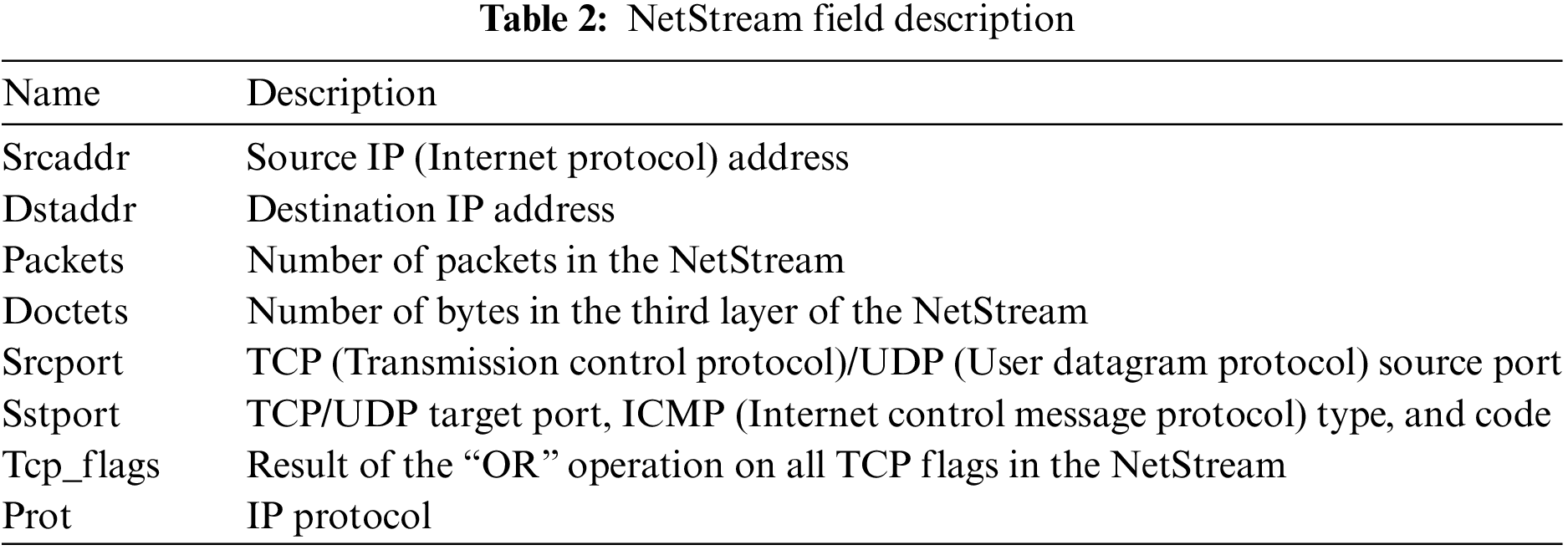
Network behavior within the context of modern network technology refers to the intentional actions of users utilizing electronic networks facilitated by computer systems to achieve specific objectives. The characterization of network user behavior can be approached from various perspectives. This study adopted the NetStream perspective to delineate user network behavior, termed the network user behavior flow. Utilizing Huawei’s NetStream flow [34] statistics tool, this study collected streams encompassing the rich attributes of user behavior flows. Subsequent analysis was conducted based on data collected through NetStream statistical flows. Table 2 provides descriptions of the fields within NetStream, which are essential for constructing network behavior streams from NetStream viewpoints.

2.5.2 Analysis and Feature Extraction of NetStream

Common representations of network user behavior include quadruples consisting of the source IP, destination IP, statistical parameters, and their corresponding values [35]. The selection of statistical parameters is contingent upon the research purpose, with popularity serving as an indicator of network user behavior within the flow. This study focused on delineating the characteristics of network user behavior within a flow. It conducted an analysis of flow characteristics pertaining to normal user online behavior using sampled traffic data, referencing the findings described in [36], to construct a feature set for user behavior based on NetStream flow data [37]. The resulting trends are shown in Table 3, which illustrates the characteristic traits.

3  Clustering Method Based on a Gravity Algorithm

3.1 Clustering Algorithm

The clustering algorithm, an unsupervised learning method, categorizes similar data objects within a dataset into groups or classes. Its objective is to maximize the similarity among objects within the same group, while minimizing the similarity between different groups. This versatile algorithm has applications across diverse domains, including data mining, machine learning, image processing, and natural language processing. It facilitates the exploration of data structures and features, revealing hidden patterns and insights within the data.

The classification of clustering algorithms encompasses partition-based, hierarchical, and density-based methods. Among these, partition-based clustering algorithms divide data into K clusters and determine the number and shape of clusters by minimizing the distance between the data points and centroids of each cluster. A typical example is K-means. Hierarchical clustering algorithms construct a hierarchical tree graph by iteratively merging or splitting data points, facilitating partitioning into any number of clusters. Cohesive hierarchical clustering is a common approach. Density-based clustering algorithms cluster data based on the density of data points, with DBSCAN (Density-Based Spatial Clustering of Applications with Noise) being a common algorithm.

Clustering algorithms offer the advantage of automatically discovering potential patterns and outliers within data, making them well suited for processing extensive datasets without requiring prior labeling. However, there are drawbacks, including challenges in meeting timeliness and accuracy requirements for clustering large-scale datasets, difficulties in directly processing mixed attribute data, dependency of clustering results on parameters, parameter selection primarily relying on experience or exploration, and lack of simple and universal methods. Hence, selecting clustering algorithms requires a comprehensive evaluation based on specific data characteristics and application scenarios.

In practical applications, such as intrusion detection, swift processing of vast amounts of data is imperative, often involving mixed attributes. In response to these characteristics and shortcomings of existing clustering algorithms, this study investigated novel clustering representation models and dissimilarity measurement methods. Consequently, a universal gravity clustering algorithm tailored for large-scale datasets with mixed attributes was proposed.

3.2 Analytical Model

This study presented a method for detecting abnormal behavior based on the universal gravitation clustering. The outlier analysis process for this model can be summarized as follows. First, a training dataset was created using the original dataset. Because an imbalance of abnormal behavior data could affect the accuracy of the classifier in complex network environments, an appropriate sampling technique was employed to balance the distribution of abnormal behavior data and enhance the accuracy of identifying such behaviors. Subsequently, a similarity or distance measure was applied to measure the similarity between data objects with the aim of assigning objects that were similar to the same cluster with the difference minimized within a cluster. Finally, a process for user-outlier detection and analysis was established. The outlier detection module and misuse detection method contributed to enhancing recognition accuracy, and a response module was integrated. The abnormal user behavior cluster analysis model is shown in Fig. 3.

Figure 3: User abnormal behavior cluster analysis model

3.3 Related Definitions

The clustering-based outlier mining algorithm can expand the definition of distance into a more general difference definition. Drawing upon Definitions 10 and 11, this study employed the concept of universal gravitation to propose a unique definition of difference, thereby establishing an abnormal user mining approach grounded in universal gravitation.

Definition 13: The difference (or dissimilarity) between clusters C1 and C2 is defined as:

dissim(C1,C2)=d(C1,C2)ln⁡(|C1|+9)⋅ln⁡(|C2|+9)(55)

In particular, the difference between object p and cluster C is:

dissim(p,C)=d(p,C)ln⁡(10)⋅ln⁡(|C|+9)(56)

Definition 14: Suppose that C={C1,C2,⋯,Ck} is a division of D, that is D=∪i=1kCi (Ci∩Cj=∅,i≠j).

The outlier factor OF(Ci) of cluster Ci is defined as the average difference between Ci and all clusters:

OF(Ci)=∑j≠idissim(Ci,Cj)k−1(57)

dissim(Ci,Cj) can be regarded as the degree to which Ci deviates from Cj. It can be seen from the definition that this degree of deviation not only reflects the relative distance between clusters, but also considers the size of the cluster. OF(Ci) measures the degree to which cluster Ci deviates from the entire dataset. The greater the value, indicating that the farther Ci deviates from the whole.

3.4 Algorithm Description

3.4.1 Clustering Algorithm

The minimum difference principle was utilized to cluster the data. The specific process is as follows:

(1) Initially, the cluster collection is empty before a new object is read in.

(2) A new cluster is created using this object.

(3) If the end of the data is reached, the algorithm terminates. Otherwise, a new object is read in. By employing the difference criterion, the disparity between the new object and each existing cluster is determined, and the least dissimilarity is selected.

(4) If the minimum difference exceeds the given threshold r, return to (2).

(5) Otherwise, the object is merged into the cluster with the smallest difference, updating the statistical frequency of each classification attribute value of the class and centroid of the numerical attribute. Return to (3).

(6) The algorithm terminates.

3.4.2 Abnormal User Detection

The initial stage employed a clustering algorithm based on the minimum difference principle to group data. The subsequent stage proceeded by initially calculating the abnormality factor for each cluster, subsequently arranging the clusters in descending order based on their abnormality factor, and ultimately designating the abnormal cluster, that is, the abnormal user. The specific explanation is as follows:

Phase 1

Clustering: Cluster the dataset D and obtain the clustering result C={C1,C2,⋯,Ck}.

Phase 2

Determining the abnormal cluster: Calculate the outlier factor OF(Ci) of each cluster Ci(1≤i≤k); rearrange Ci(1≤i≤k) in the decreasing order of OF(Ci); find the minimum b that satisfies ∑i=1b|Ci||D|≥ε(0<ε<1); and mark clusters C1,C2,⋯,Cb as ‘outlier’ (that is, each object in it is regarded as outlier), and mark Cb+1,Cb+2,⋯,Ck as the normal cluster ‘normal’ (that is, each object in it is regarded as normal), where b can also be directly determined by prior knowledge.

3.5 Time and Space Complexity Analysis

The performance of the clustering algorithm with respect to time and space complexity can be influenced by several factors, including the size of the dataset N, the number of attributes m, the number of clusters generated, and the size of each cluster. To facilitate the analysis, it can be assumed that the number of clusters finally generated is k, and that each classification attribute D has n distinct values. In the worst case, the time complexity of the clustering algorithm is:

O(N⋅k(∑i=1mcni+mN))(58)

The space complexity is:

O(N⋅m+k(∑i=1mcni+mN))(59)

As the clustering algorithm is executed, the number of clusters progressively expands from 1 to k concurrently with an increase in the number of attribute values within the clusters. It has been highlighted in [30] that categorical attributes typically exhibit an exceedingly small value range. The customary range of categorical attribute values is less than 100 distinct values, and ∑i=1mcni can typically fall within a restricted range. Therefore, in practical scenarios, the anticipated time complexity of the clustering algorithm is:

O(N⋅k⋅m)(60)

4  Experimental Analysis and Results

4.1 Experimental Parameters

To assess whether user behavior was abnormal by comparing it to a database of abnormal behavior using the Euclidean distance, it was required to determine a suitable range for the threshold value r. To begin this process, N0 pairs of objects within dataset D were randomly selected. Subsequently, the differences between each pair of objects were computed and the average EX of these differences was determined using Eq. (2). The value of r was set within the range [EX − 0.25D, EX + 0.23DX].

4.2 Experimental Tests

The Euclidean distance (x = 2 in Definition 7) was utilized to quantify the differences between data, and the effectiveness of the algorithm was verified on the DARPA 00 intrusion detection evaluation dataset and its extended version, Dataset 99.

4.2.1 DARPA 00 Dataset

The model was constructed using the data from week1 and week2, and subsequently evaluated using the data from the remaining 4 weeks. Table 4 presents the experimental results when threshold r was set between 0.5 and 0.6.

4.2.2 NSL KDD Dataset

The NSL KDD dataset, a revised iteration of the renowned KDD Cup 99 dataset, features both training and testing sets devoid of redundant records, thereby enhancing detection accuracy. Each dataset record comprises 43 features, with 41 representing the traffic input and the remaining two denoting labels (normal or attack) and scores (severity of the traffic input). Notably, the dataset includes four distinct attack types: Denial of Service (DoS), PROBE, User to Root (U2R), and Remote to Local (R2L). A portion of the NSL KDD dataset, comprising 10% of the data, was used to evaluate the performance of the algorithm. This subset was selected, where all 41 attributes were employed for processing. This subset were randomly divided into three groups: P1, P2, and P3. P1 contained 41,232 records, representing 96% normal accounts, P2 contained 19,539 records, representing 98.7% normal accounts, and P3 contained attack types not present in P1, including ftpwrite, guess_passw, imap, land, loadmodule, multihop, perl, phf, pod, rootkit, spy, and warezmaster.

4.3 Analysis of the Effectiveness of r

The model was trained using P1 as the training set (ε = 005). The established model was tested on P3, obtaining EX = 0.234, DX = 0.134, EX − 0.5DX = 0.17, EX − 0.25DX = 0.20, EX + 0.25DX = 0.27, and EX + 0.5DX = 0.30. Furthermore, various values of r were obtained between EX − 0.5DX and EX + 0.5DX, and the detection rates of the different types of attacks are presented in Table 5.

It can be seen that when conducting experiments on networks with different types of attacks using r, the detection results are basically stable, and the overall detection rate reaches over 90%, verifying the effectiveness of r and providing effective measurement parameters for anomaly detection algorithms. Taking into account both time efficiency (i.e., number of clusters) and accuracy, it is recommended that r be taken between EX − 025DX and EX + 0.25D.

4.4 Performance Analysis

To evaluate the performance of the universal gravitation clustering algorithm, it was necessary to compare it with existing algorithms, such as the BP neural network and nearest neighbor detection algorithm proposed in [28,34]. Fig. 4 illustrates the comparison of the three abnormal user behavior analysis methods with different numbers of training samples and test samples. The overall detection rates were improved to a certain extent as the number of test samples increased. The performance of the BP neural network algorithm was found to be unsatisfactory, owing to its susceptibility to noise and instability. Meanwhile, the nearest neighbor detection algorithm grew approximately linearly, exhibiting limited stability. It was only capable of performing fuzzy classification, without the ability to accurately identify or detect Distributed Denial of Service (DDOS) attacks. In contrast, the clustering algorithm proposed in this study had notable advantages. By employing the difference concept under the universal gravitation algorithm, the data were classified effectively even for various test samples. The overall stability of the algorithm was highest, with an average detection rate of 0.98.

Figure 4: Comparison of detection rates

Fig. 5 presents a comparative analysis of the detection speeds of the three-intrusion detection behavior analysis algorithms with varying numbers of training and test samples. As the number of test samples increased, the recognition speed of the algorithms also increased. This study utilized under-sampling to preprocess the data and employed a minimum difference principle-based clustering algorithm to cluster the data, which contributed to the increased speed of sample detection.

Figure 5: Comparison of detection speeds

Fig. 6 illustrates a comparison of the accuracies of the three user abnormal behavior analysis algorithms with respect to the number of training and test samples. As the number of test samples increased, the accuracy of the three algorithms improved to a certain extent. However, owing to the influence of noise, the accuracy of the BP neural network algorithm was unstable. The nearest neighbor-based user abnormal behavior analysis method failed to identify DDOS attacks, which adversely affected its accuracy in identifying abnormal behaviors. In contrast, the algorithm proposed in this study was resistant to noise, capable of identifying DDOS attacks, and demonstrated the potential for recognizing unknown attack types. Therefore, the algorithm presented favorable stability and high accuracy.

Figure 6: Accuracy comparison

Fig. 7 demonstrates a comparison of the false rates for the three abnormal behavior analysis methods that utilized varying numbers of training and test samples. The graph indicates that the overall false rates for the three methods decreased as the number of test samples increased. However, the method proposed in this paper, which employed an outlier identification algorithm, demonstrated a consistently lower false rate than the other two methods. This suggested that the algorithm had superior capabilities for accurately identifying abnormal user behavior.

Figure 7: False-rate comparison

Fig. 8 compares the missing rates for the three-user abnormal behavior analysis methods, based on varying numbers of training and test samples. The missing rates for all the three algorithms decreased as the number of test samples increased. However, the BP neural network algorithm was affected by noise and unidentified outlier types, resulting in a relatively high missing rate. The nearest neighbor algorithm was unable to identify DDOS attacks and could only perform fuzzy classification, leading to a high missing rate. In contrast, the algorithm proposed in this study demonstrated a lower sensitivity to noise and exhibited a certain degree of recognition for unknown attack types. Consequently, it had a lower false-negative rate than the other two algorithms.

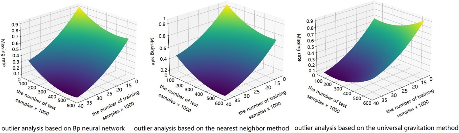
Figure 8: Missing rate comparison

Fig. 9 presents a comparison of the predicted classification results obtained using the algorithm proposed in this study with the actual classification results in the context of unknown types of abnormal behaviors. This experimental comparison indicated that the algorithm proposed in this study exhibited superior identification capabilities for known outliers and achieved more favorable classification outcomes for unknown outlier types.

Figure 9: Comparison of predicted and real classification results

The findings from the experiments conducted in this study revealed that the universal gravitation clustering method demonstrated remarkable speed in detecting abnormal behaviors while maintaining a high level of accuracy. It was also found that the algorithm was relatively resistant to noise, enabling it to utilize a semi-supervised learning technique to classify user behavior effectively. This proved to be an effective approach for identifying and responding to abnormal behaviors.

Overall, abnormal behavior analysis technology demonstrated commendable scalability and adaptability while exhibiting robust identification capabilities.

5  Conclusion

Considering the limitations of traditional clustering algorithms in addressing real-time requirements for high-dimensional data, this study presented a method for detecting abnormal behavior based on a universal gravitation clustering algorithm. The algorithm demonstrated exceptional stability with an average detection rate of 0.98. First, the minimum difference principle-based clustering algorithm was employed to cluster the data, followed by calculation of the outlier factor for each cluster. The clusters were then sorted according to the outlier factors, enabling the identification of abnormal users in the network. The simulation results demonstrated that this method exhibited notable improvements in detection rate, speed, false rate, and missing rate. In summary, the proposed intrusion detection method based on a universal gravitation clustering algorithm offers numerous advantages, effectively addresses evolving network intrusion threats, and contributes to the protection of network system security.

The algorithm addresses the challenges in parameter settings within traditional clustering methods. This study provides comprehensive insights into the fundamental principles, parameter settings, clustering evaluation criteria, and algorithmic steps. Practical applications demonstrated its efficacy in both clustering analysis and anomaly detection. However, implementation and performance may vary owing to factors such as dataset scale, dimensionality, abnormal behavior definitions, and detection thresholds. Despite this, the anomaly detection method based on the law of universal gravitation clustering algorithms proved to be effective in practical applications, exhibiting excellent clustering and anomaly detection capabilities. Nevertheless, implementation specifics necessitate the evaluation and optimization tailored to distinct application scenarios and datasets. With the continuous development of big data and machine learning technologies, there is significant potential for advancing anomaly detection methods utilizing the law of universal gravitation clustering algorithms. For instance, incorporating deep learning techniques can enhance the capability of the algorithm to handle complex data, whereas integrating other anomaly detection methods can yield a more comprehensive and accurate anomaly detection system.

Acknowledgement: The authors would like to thank all the reviewers who participated in the review, as well as MJEditor (www.mjeditor.com) for providing English editing services during the preparation of this manuscript.

Funding Statement: YJ, YGF, XXM, and LZX are supported by the Fujian China University Education Informatization Project (FJGX2023013). National Natural Science Foundation of China Youth Program (72001126). Sanming University’s Research and Optimization of the Function of Safety Test Management and Control Platform Project (KH22097). Young and Middle-Aged Teacher Education Research Project of Fujian Provincial Department of Education (JAT200642, B202033).

Author Contributions: The authors confirm their contribution to the paper as follows: Study conception design: Jian Yu, Gaofeng Yu, Xiangmei Xiao, Zhixing Lin; data collection: Jian Yu, Xiangmei Xiao, Zhixing Lin; analysis and interpretation of results: Jian Yu, Xiangmei Xiao; draft manuscript preparation: Jian Yu, Gaofeng Yu. All authors reviewed the results and approved the final version of the manuscript.

Availability of Data and Materials: Due to the nature of this research, participants of this study did not agree for their data to be shared publicly, so supporting data is not available.

Conflicts of Interest: The authors declare that they have no conflicts of interest to report regarding the present study.

References

1. S. Bhattacharya et al., “A novel PCA-fireflbased XGBoost classification model for intrusion detection in networks using GPU,” Electronics, vol. 2, no. 19, pp. 219–327, 2020. [Google Scholar]

2. R. M. S. Priya et al., “An effectivefeature engineering for DNN using hybrid PCA-GWO for intrusion detection,” IoMT Architect. Comput. Commun., vol. 160, no. 23, pp. 139–149, 2020. [Google Scholar]

3. S. Namasudra, R. Chakraborty, A. Majumder, and N. R. Moparthi, “Securing multimedia by using DNA-based encryption in the cloud computing environment,” ACM Trans. Multimed. Comput. Commumn. App., vol. 16, no. 3s, pp. 1–19, 2020. doi: 10.1145/3392665. [Google Scholar] [CrossRef]

4. R. Alkanhel et al., “Network intrusion detection based on feature selection and hybrid metaheuristic optimization,” Comput., Mater. Contin., vol. 74, no. 2, pp. 2677–2693, 2023. doi: 10.32604/cmc.2023.033273. [Google Scholar] [CrossRef]

5. F. M. Alotaibi, “Network intrusion detection model using fused machine learning technique,” Comput., Mater. Contin., vol. 75, no. 2, pp. 2479–2490, 2023. doi: 10.32604/cmc.2023.033792. [Google Scholar] [CrossRef]

6. S. Sharma, V. Kumar, and K. Dutta, “Multi-objective optimization algorithms for intrusion detection in IoT networks: A systematic review,” Internet Things Cyber-Phys. Syst., vol. 56, no. 4, pp. 4258–4267, 2024. [Google Scholar]

7. B. L. Li, L. Zhu, and Y. Liu, “Research on cloud computing security based on deep learning,” Comput. Knowl. Technol., vol. 45, no. 22, pp. 166–168+174, 2019 (In Chinese). [Google Scholar]

8. D. Ravikumar et al., “Analysis of smart grid-based intrusion detection system through machine learning methods,” Int. J. Electr. Secur. Digit. Forensic., vol. 16, no. 2, pp. 84–96, 2024 (In Chinese). [Google Scholar]

9. S. N. Samina Khalid and T. Khalil, “A survey of feature selection and feature extraction techniques in machine learning,” in 2014 Sci. lnform. Conf., London, UK, 2017, vol. 24, pp. 1–13. [Google Scholar]

10. S. Musyimi, M. Waweru, and C. Otieno, “Adaptive network intrusion detection and mitigation model using clustering and bayesian algorithm in a dynamic environment,” Int. J. Comput. App., vol. 181, no. 20, pp. 36–48, 2018. [Google Scholar]

11. H. Ngo et al., “Federated fuzzy clustering for decentralized incomplete longitudinal behavioral data,” IEEE Internet Things J., vol. 11, no. 8, pp. 14657–14670, 2024. doi: 10.1109/JIOT.2023.3343719. [Google Scholar] [CrossRef]

12. S. Iqbal and C. Zhang, “A new hesitant fuzzy-based forecasting method integrated with clustering and modified smoothing approach,” Int. J. Fuzz. Syst., vol. 22, no. 4, pp. 1–14, 2020. [Google Scholar]

13. Y. Sun et al., “Dynamic intelligent supply-demand adaptation model towards intelligent cloud manufacturing,” Comput., Mater. Contin., vol. 72, no. 2, pp. 2825–2843, 2022. doi: 10.32604/cmc.2022.026574. [Google Scholar] [CrossRef]

14. Z. Abdulmunim Aziz and A. Mohsin Abdulazeez, “Application of machine learning approaches in intrusion detection system,” J. Soft Comput. Data Min., vol. 2, no. 2, pp. 1–13, 2021. [Google Scholar]

15. B. Ingre, A. Yadav, and A. K. Soni, “Decision tree based intrusion detection system for NSL-KDD dataset,” in Inf. Commun. Technol. Intell. Syst., Springer, 2017, pp. 207–218. [Google Scholar]

16. S. Aljawarneh, M. Aldwairi, and M. B. Yassein, “Anomaly-based intrusion detection system throughfeature selection analysis and building hybrid efficient model,” J. Comput. Sci., vol. 25, no. 6, pp. 152–160, 2018. [Google Scholar]

17. C. Yin et al., “A deep learning approach for intrusion detection using recurrentneural networks,” IEEE Access, vol. 5, pp. 21954–21961, 2017. doi: 10.1109/ACCESS.2017.2762418. [Google Scholar] [CrossRef]

18. U. Ahmad, H. Asim, M. T. Hassan, and S. Naseer, “Analysis of classification techniques for intrusion detection,” in 2019 Int. Conf. Innov. Comput., New Delhi, India, IEEE, 2019, pp. 1–6. [Google Scholar]

19. S. A. Aziz, E. Sanaa, and A. E. Hassanien, “Comparison of classification techniques applied fornetwork intrusion detection and classification,” J. Appl. Logic., vol. 24, pp. 109–118, 2017. doi: 10.1016/j.jal.2016.11.018. [Google Scholar] [CrossRef]

20. A. Hajimirzaei and N. J. Navimipour, “Intrusion detection for cloud computing using neural networks and artificial bee colony optimization algorithm,” ICT Express, vol. 5, no. 1, pp. 56–59, 2019. doi: 10.1016/j.icte.2018.01.014. [Google Scholar] [CrossRef]

21. M. R. Parsaei, S. M. Rostami, and R. Javidan, “A hybrid data mining approach for intrusion detectionon imbalanced NSL-KDD dataset,” Int. J. Adv. Comput. Sci. App., vol. 7, no. 6, pp. 20–25, 2016. [Google Scholar]

22. Y. S. Sydney and M. Kasongo, “A deep learning method with wrapper based feature extraction for wireless intrusion detection system,” Comput. Secur., vol. 92, pp. 101752, 2020. doi: 10.1016/j.cose.2020.101752. [Google Scholar] [CrossRef]

23. K. E. S. Hadeel Alazzam and A. Sharieh, “A feature selection algorithm for intrusion detection system based on pigeon inspred optimizer,” Expert. Syst. App., vol. 148, pp. 113249, 2020. doi: 10.1016/j.eswa.2020.113249. [Google Scholar] [CrossRef]

24. J. Singh and M. J. Nene, “A survey on machine learning techniques forintrusion detection systerns,” Int. J. Adv. Res. Comput. Commun. Eng., vol. 12, no. 1, pp. 4349–4355, 2013. [Google Scholar]

25. F. C. Tsai et al., “Intrusion detection by machine learning: A review,” Expert. Syst. App., vol. 36, no. 10, pp. 11994–12000, 2002. [Google Scholar]

26. J. R Quinlan, “Induction of decision trees,” Mach. Leam., vol. 1, no. 1, pp. 81–106, 1986. doi: 10.1007/BF00116251. [Google Scholar] [CrossRef]

27. Y. Z. Zhu, “Intrusion detection method based on improved BP neural network research,” Int. J. Secur. App., vol. 10, no. 5, pp. 193–202, 2016. [Google Scholar]

28. H. Zhao, Y. Jiang, and J. Wang, “Cloud computing user abnormal behavior detection method based on fractal dimension clustering algorithm,” J. Intell. Fuzz. Syst., vol. 37, no. 1, pp. 1103–1112, 2019. [Google Scholar]

29. A. M. Yogita Hande, “A survey on intrusion detection system for software defined networks (SDN),” in Research Anthology on Artificial Intelligence Applications in Security, 2021. doi: 10.4018/978-1-7998-7705-9.ch023. [Google Scholar] [CrossRef]

30. K. S. Dorman and R. Maitra, “An efficient k-modes algorithm for clustering categorical datasets,” Stat. Analy. Data Min, vol. 15, no. 1, pp. 83–97, 2022. doi: 10.1002/sam.v15.1. [Google Scholar] [CrossRef]

31. Y. Gao, Y. Hu, and Y. Chu, “Ability grouping of elderly individuals based on an improved K-prototypes algorithm,” Mathemat. Probl. Eng., vol. 56, no. 23, pp. 1–11, 2023. [Google Scholar]

32. R. S. Sangam and H. Om, “An equi-biased k-prototypes algorithm for clustering mixed-type data,” Sādhanā, vol. 43, no. 3, pp. 37, 2018. doi: 10.1007/s12046-018-0823-0. [Google Scholar] [CrossRef]

33. F. Gholamreza, “Black hole attack detection using K-nearest neighbor algorithm and reputation calculation in mobile ad hoc networks,” Secur. Commun. Netw., vol. 2021, pp. 1–15, 2021. [Google Scholar]

34. Y. Hu, X. Chen, and J. Wang, “Abnormal traffic detection based on traffic behavior characteristics,” Inf. Netw. Secur., vol. 57, no. 11, pp. 45–51, 2016. [Google Scholar]

35. T. Qin et al., “Users behavior character analysis and classification approaches in enterprise networks,” in IEEE. Eighth IEEE/ACIS Int. Conf. Comput. Inf. Sci., Shanghai, China, 2009, pp. 323–328. [Google Scholar]

36. V. C. Adrián et al., “Malicious traffic detection on sampled network flow data with novelty-detection-based models,” Sci. Rep., vol. 13, no. 1, pp. 15446, 2023. doi: 10.1038/s41598-023-42618-9. [Google Scholar] [CrossRef]

37. J. Guo, D. Li, and Z. Chen, “Performance analysis of heterogeneous traffic networks based on sFlow and NetStream,” Int. J. Perform. Eng., vol. 16, no. 10, pp. 1598–1607, 2020. doi: 10.23940/ijpe.20.10.p11.15981607. [Google Scholar] [CrossRef]