Maximum Power Point Tracking Control of Offshore Wind-Photovoltaic Hybrid Power Generation System with Crane-Assisted

1  Introduction

1.1 Background of the Topic and Research Significance

With the rapid development of global industry and economy, countries are increasingly dependent on fossil energy. This deep-seated dependence has not only led to the gradual depletion of resources, but also caused irreversible pollution and damage to the environment. For China, which is in a period of rapid development, this situation is even more grim. According to relevant data, China has become the world’s largest energy producer and consumer. Therefore, in order to solve the energy crisis and achieve high-quality development, China must get rid of its excessive dependence on non-renewable fossil energy. In contrast, renewable energy has the advantages of being pollution-free, abundant in reserves and widely distributed. It will be an ideal substitute for fossil energy and the key to China’s entry into a new stage of development [1].

The wind power-photovoltaic complementary power generation system has great technical and economic feasibility and the ability to reduce wind and solar power abandonment. Among many renewable energy sources, solar energy and wind energy are highly favored due to their abundant resources and low cost. Regarding wind energy, in the 10 m low-altitude area, the total amount of onshore exploitable energy in China is 253 million kW; in the 80, 100, 120 and 140 m high-altitude areas, the total amount of onshore wind energy resources technically developed in China is 3.2, 3.9, 4.6 and 5.1 billion kW, respectively. Regarding solar energy, China’s annual total solar radiation is roughly between 3344 and 8400 MJ/m2, and more than two-thirds of the regions have annual sunshine hours greater than 2000 h. According to the 2023 China Wind and Solar Energy Resources Annual Bulletin, the distribution of the average wind power density and total horizontal irradiation at 100 m on land in China [2].

It can be seen that China’s wind and solar energy resources have a high degree of consistency in regional distribution, mainly concentrated in the western region. These places are vast and sparsely populated, which is very suitable for the construction of large-scale wind farms and offshore photovoltaic power plants. In view of the rich offshore wind and solar resources and convenient construction conditions, China is constantly expanding the installed capacity of offshore wind and solar power generation. By the end of October 2023, China’s total installed capacity of renewable energy power generation exceeded 1.4 billion kW, a year-on-year increase of 20.8%, accounting for about 49.9% of China’s total installed capacity, of which wind power has reached 390 million kW and offshore photovoltaic power generation has reached 536 million kW. By 2025, China’s total installed power capacity will reach 2.95 billion kW, of which wind and photovoltaic installed capacity will reach 540 and 560 million kW, respectively [3].

Therefore, offshore photovoltaic power generation, offshore wind power generation and offshore energy storage systems can be combined to form an offshore wind-solar complementary power generation system, which can weaken the impact of environmental factors on power generation, thereby making the system more stable and reliable. Although the offshore wind-solar complementary power generation system can achieve output power complementarity on a seasonal and day-night time scale, the maximum output power point of the power generation system will also fluctuate at all times due to the constant fluctuations in wind speed and light intensity. This study is motivated by the urgent need to explore how hybrid renewable energy systems (HRES) can address the limitations inherent in single-source systems. By delving into technical challenges, economic considerations, and policy prospects, this study aims to provide a comprehensive overview to guide future research, investment, and policy development in this area. If the power generation system is not controlled to track the maximum power point in real-time, the power generation efficiency will become low. Therefore, in order to improve the power generation efficiency, it is very necessary to design an efficient and reasonable maximum power point tracking (MPPT) control method.

1.2 Research Status of Offshore Wind-Solar Hybrid Power Generation System

Power prediction can be used as a reference for control strategies and capacity configuration, which helps to improve the power generation efficiency of the entire power generation system. At present, research in this field mainly focuses on the use and improvement of various neural network models. Wei et al. analyzed the output of wind power and offshore photovoltaic units in offshore wind-solar hybrid power stations, and proposed a neural network power prediction model based on an improved dynamic group cooperation optimization algorithm, which effectively reduced the prediction error [4]. Liu et al. used a wavelet neural network for power prediction of offshore wind-solar hybrid systems. Since wavelet analysis has advantages in extracting signal features and analyzing non-stationary signals, the prediction accuracy of the model can be improved by combining the adaptive ability and self-learning ability of artificial neural networks [5]. The groundbreaking ceremony of the 1600 T self-propelled self-elevating wind turbine installation fully revolving crane vessel built by Zhenhua Heavy Industries for China Power Construction was held in Nantong Zhenhua Heavy Equipment. The 1600 T self-propelled self-elevating wind turbine installation platform has a total length of 123.95 m, a beam of 48 m, a depth of 9.5 m, and a cruising range of 3000 nautical miles. Its lifting capacity is 1600 t, the operating water depth is 70 m, the variable load is not less than 5000 t, and the operating deck area is 3500 square meters. It has lifting, transportation, storage and other functions, and is suitable for unlimited navigation areas. It can meet the needs of deep-sea integrated offshore wind turbine construction operations. The ship is mainly used for offshore wind turbine installation and can transport 2 sets of 12 MW wind turbine equipment and large foundation pipe piles at a time [6]. On 6 April 2024, off the coast of Laizhou Bay in Yantai City, Shandong Province, China, the CGN Yantai Zhaoyuan 400 MW offshore photovoltaic project was under construction at sea. The project is China’s first large-scale fixed offshore photovoltaic project. The first superstructure equipped with solar panels is installed on support piles driven into the seabed. The superstructure is about 70 m long, 40 m wide, weighs 120 t, has an installed capacity of approximately 0.59 MW, and is 17.3 m above the water surface after installation. The offshore installation work was carried out by the 500-t offshore photovoltaic panel crane “Lifting 19” [7].

Marzebali et al. considered the instability of the frequency of an independent offshore wind-solar hybrid AC (Alternating Current) microgrid, proposed a hybrid offshore energy storage system that combines fuel cells and batteries, and used a dynamic droop control strategy to coordinate the power distribution between the two. The hybrid offshore energy storage system and control strategy improve the stability of the AC bus voltage frequency and the life of the battery. When the offshore energy storage system stops working, the offshore wind-solar power generation system assumes the role of maintaining stable voltage and power, but in most cases it is in the Maximum Power Point Tracking (MPPT) state. In the offshore wind-solar hybrid power generation system, the most commonly used MPPT control method is to perform independent MPPT control on the wind power and offshore photovoltaic power generation systems [8]. Liao et al. studied the MPPT control of grid-connected offshore wind-solar hybrid power generation systems, using an adaptive conductance increment method for offshore photovoltaic power generation and an adaptive perturbation observation method for offshore wind power generation. These methods improve the convergence speed while reducing steady-state power oscillations [9]. Liang et al. proposed a two-layer capacity optimization model based on an offshore wind-solar hybrid power generation system that integrates solar thermal power stations and offshore energy storage, and configured and scheduled it through the locust algorithm and Cplex solver. This capacity optimization configuration method alleviates peak load demand and improves the economy and configuration rationality of the system [10]. These research fields are constantly progressing, providing technical support for the development of offshore wind-solar hybrid systems and promoting the wider application of renewable energy. The MPPT control method determines the power generation efficiency of the system during normal operation. Therefore, this study will focus on the core area of MPPT control.

1.3 Research Status of MPPT Control Methods for Offshore Wind-Solar Hybrid Power Generation Systems

There are four main methods for traditional MPPT tracking control strategies for offshore wind power generation systems: tip speed ratio method, hill climbing search method, power signal feedback method and optimal torque method. At present, scholars from various countries have also developed some new MPPT control algorithms with the help of modern control and intelligent algorithms. Traditional MPPT control strategies achieve maximum power point tracking from different operating characteristics of offshore wind power generation systems, so each algorithm has its own characteristics and advantages and disadvantages.

(1)   The hill climbing search method mainly uses the curve relationship between output power and mechanical angular velocity. For a certain wind speed, there is only one maximum power point corresponding to it. If the mechanical angular velocity is continuously adjusted by the change in the output power of the offshore wind turbine and the change in the mechanical angular velocity, the offshore wind power generation system can be close to the maximum power point of the wind speed. Although the hill climbing search method can be independent of external conditions, it is only applicable to situations where the wind speed changes slowly and requires precise adjustment of the search step size to achieve the best effect. Youssef et al. divided the power-to-angular velocity curve into several different sectors and used an adaptive hill-climbing search method near the maximum power point to balance the contradiction between low oscillation and fast tracking. However, the zoning standard is difficult to determine because changes in wind speed will lead to different ranges of mechanical angular velocity changes, and the change trend is not linear [11].

(2)   The power signal feedback method and the optimal torque method mainly use the optimal power curve and the optimal torque curve to control the corresponding physical quantities, thereby realizing maximum power point tracking. In the control process, the power signal feedback method and the optimal torque method only need to monitor the two parameter variables of the real-time mechanical angular velocity and output power of the offshore wind turbine, which has a certain simplicity. However, its overall tracking speed depends on the system inertia, and the optimal curve it relies on is easily disturbed by external conditions, so its application scope is limited in actual engineering applications. Prabhakar et al. aimed to explore several inertia estimation (IE) methods, trying to discover the main difficulties and main characteristics of various IE algorithms, and discussed the future directions and possibilities of IE [12]. Hong et al. designed an optimal torque compensator based on gradient estimation to compensate for the given value of the electromagnetic torque to reduce the influence of large rotational inertia on the change of the mechanical angular velocity of the offshore wind turbine. This method has good system stability and dynamic characteristics, and the transient process time is short. Although this method increases the tracking speed, the tracking accuracy cannot be guaranteed because it still relies on the optimal curve, which is not fixed during operation and is easily disturbed [13].

From the above data, it can be seen that there are roughly three directions for improving MPPT control of offshore wind power generation: one is to combine traditional algorithms to form complementary advantages; the second is to improve the performance of the controller based on the traditional algorithm; the third is to use intelligent algorithms to directly replace and improve the traditional method. For the tip speed ratio method, its biggest disadvantage is the increased cost of wind speed sensors and the complexity of wind speed measurement. However, with the development of technology, the cost of wind speed sensors is decreasing and the accuracy is also increasing. In this case, the first method will increase the computational burden, and the advantage of the third method is not particularly obvious. Therefore, it is a better solution to improve the control performance based on the tip speed ratio method. Among the common control algorithms, neural networks have high computational costs due to the need for a large amount of data for pre-training; fuzzy control relies on expert experience and is suitable for situations where the control accuracy requirements are not too high, so it is not suitable for the problem of maximum power point tracking; although there is a chattering problem in sliding mode control, its sliding mode control has the advantages of simple implementation, strong anti-interference ability, and fast convergence. In summary, for the MPPT control of offshore wind power generation systems, this study will study the sliding mode control algorithm based on the tip speed ratio method. The total length of Zhenhua Heavy Industries’ 3600T fully revolving offshore wind turbine-photovoltaic crane ship is 182 m, the width is 49 m, and the depth is 15 m. A heavy offshore crane with a lifting capacity of 3600 t × 40 m (fixed tail crane)/3000 t × 45 m (fully revolving) is installed at the stern, which can carry out offshore wind turbine-photovoltaic lifting and installation operations. The ship is suitable for sailing in unlimited navigation areas, mainly for offshore wind turbine-photovoltaic piling and installation, while taking into account the lifting and installation of marine structures. The picture of Zhenhua Heavy Industries’ 3600T fully revolving offshore wind turbine-photovoltaic crane ship is shown in Fig. 1 [14].

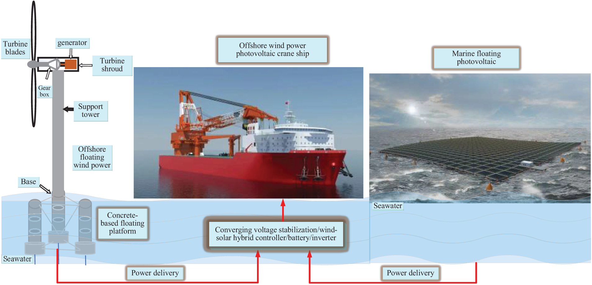
Figure 1: Zhenhua Heavy Industries’ 3600T fully revolving offshore wind turbine-photovoltaic crane shipwith offshore crane-assisted

1.4 Research Status of MPPT Control of Offshore Photovoltaic Power Generation System

Under different lighting conditions, the output power and voltage (P-U) curve of the offshore photovoltaic array will show different characteristics: when the light intensity is uniform, the P-U curve of the offshore photovoltaic array has only one global maximum peak; when the light intensity is uneven, such as due to factors such as building shading and clouds, the P-U curve of the offshore photovoltaic array will have multiple peaks.

(1)   The principle of the perturbation observation method is similar to the hill climbing search method of wind power, but the physical quantity of the perturbation is different. The algorithm first applies a perturbation to the output voltage of the offshore photovoltaic array, measures the voltage and current to calculate the power, and compares it with the previous moment. Then, the perturbation direction is determined according to the power change. Finally, repeating this process continuously can make the system approach the maximum power point. This method has the advantages of easy implementation and fewer measurement parameters, but its perturbation step size is difficult to determine: if it is too small, the tracking speed will be slow; if it is too large, the steady-state oscillation will be too large, thus affecting the power generation efficiency of the system. Mohamedy Ali et al. proposed an improved perturbation and observation algorithm, which first partitions the P-U curve of the offshore photovoltaic system and then tracks the maximum power point by combining large and small step sizes. This method not only achieves fast tracking but also reduces steady-state oscillations, but the partitioning criteria are difficult to determine [15].

(2)   The conductance increment method is a method that uses the relationship between the instantaneous conductance and dynamic conductance of the offshore photovoltaic array to adjust the control signal of the system. Its purpose is to find the point where dP/dU = 0, and by continuously changing the duty cycle of the PWM control signal, the offshore photovoltaic array can output the maximum power at the maximum power point. The conductance increment method has a good tracking effect under uniform illumination conditions. Compared with the perturbation observation method and the constant voltage method, the algorithm has a smaller oscillation amplitude and higher accuracy when reaching a steady state, but the perturbation step size still needs to be reasonably selected. Li et al. proposed a new variable step size algorithm. According to the slope change law of the P-U curve of offshore photovoltaic cells, the algorithm uses logarithmic and exponential function values as dynamic step size coefficients, combines the constant voltage coefficient method to obtain the initial step size value, and uses the power correction method to avoid misjudgment caused by sudden environmental changes. These improvements can enable the offshore photovoltaic power generation system to find the maximum power point faster, while effectively reducing the power loss caused by step size oscillation, but may fail when the illumination conditions change rapidly [16].

Shangguan et al. proposed an improved gray wolf optimization algorithm to deal with the multi-peak problem under local shadows. The algorithm adopted a novel nonlinear update strategy for the convergence factor of the gray wolf optimization algorithm, and introduced Levy flight and dynamic weighting strategies in the group positioning update equation [17]. Jin et al. proposed a maximum power tracking technology that combines the gray wolf optimization algorithm and the conductance increment method. The algorithm first performs a global search through the gray wolf algorithm, and then performs a local fine search using the conductance increment method [18]. Elbaksawi et al. proposed a hybrid method that combines cuckoo search and gray wolf optimization algorithm to optimize the MPPT of offshore photovoltaic power generation systems under non-uniform conditions, which not only reduces steady-state oscillations but also shortens the convergence time [19]. Ding et al. proposed a data-driven power system security situation awareness that can monitor and assess the security status of the power system and warn the organization when the system encounters suspicious threats [20].

(3)   MPPT for offshore wind-photovoltaic hybrid power systems uses intelligent algorithms or combines various control strategies according to the control needs of the power system to complement each other’s strengths and weaknesses to achieve the optimal control effect. They are very suitable for nonlinear control systems with high uncertainty. Some novel research work has been carried out, for example, Ahmed et al. studied hybrid wind and PV by integrating a buck-boost converter with a microcontroller system to achieve a consistent DC bus voltage, and a MATLAB model was developed to simulate the grid integration of hybrid wind and PV, enabling a detailed analysis of the performance of the integrated grid [21]. AL-Wesabi et al. proposed a hybrid photovoltaic/wind energy conversion system (PV/WECS) to supply and support the utility grid and proposed a novel linear active disturbance rejection control (LADRC) combined with a hybrid Salp particle swarm algorithm (SPSA) for grid-connected PV/WECS to extract the global maximum power (GMP), regulate the DC link voltage, and enhance active and reactive power control [22]. Bassey discussed the application of machine learning (ML) techniques in hybrid renewable energy systems, integrating data from solar and wind to predict system performance and improve energy storage solutions. Machine learning-driven modeling significantly improves the accuracy of hybrid renewable energy system performance predictions [23]. Chrifi-Alaoui et al. studied different configurations of hybrid solar and wind energy conversion systems. The behavior of each system was investigated, as well as their mathematical models, characteristics and existing topologies. Control strategies, optimal configurations and sizing techniques for these hybrid photovoltaic-wind systems were presented, as well as different energy management strategies [24].

From the above data analysis, it can be seen that for MPPT under a single peak, although the conductance increment method also needs to reasonably select the perturbation step size, compared with the perturbation observation method and the constant voltage method, the algorithm has a smaller oscillation amplitude and higher accuracy when reaching steady state. For MPPT under multiple peaks, the metaheuristic algorithm does not rely on the original model compared with the two-step method and the equal power curve method, so it has strong applicability. Most of the improvements to the metaheuristic algorithm in the data are concentrated in the following categories: the combination of metaheuristic algorithm and single peak algorithm, the combination of multiple metaheuristic algorithms, and the internal improvement of metaheuristic algorithm. Among them, the combination of metaheuristic algorithm and single peak algorithm can avoid random trial and error of the algorithm in the later stage, thereby improving stability and reducing computational burden, so it is a better solution. Moreover, among the above metaheuristic algorithms, the gray wolf optimization algorithm has certain advantages in tracking accuracy and speed, as well as the number of parameters. In summary, for the MPPT control of offshore photovoltaic power generation systems, this study will carry out further research on the basis of the gray wolf optimization algorithm and the conductance increment method.

1.5 Innovative Research Content Structure

This study mainly focuses on the MPPT control of offshore wind-solar hybrid power generation systems. First, the existing MPPT control methods of wind and solar power generation systems are analyzed, and then the main components and operating characteristics of offshore wind-solar hybrid power generation system are studied. Finally, based on the original MPPT control method, this study proposes new improved MPPT control algorithms for wind and solar power generation systems, and conducts a series of simulation verifications. The structure of the article is arranged as follows:

This paper is organized as follows. Section 1 mainly analyzes the significance of this study and the development of related technologies. The focus is on analyzing the current status of research on offshore wind-solar hybrid power generation system and its MPPT control, and on this basis, the technical route of this study is determined. Section 2 mainly studies the MPPT control algorithm of offshore wind power generation system. In order to improve the tracking efficiency of offshore wind power generation system to the maximum power point, a new global fast integral sliding mode control algorithm (GFISMC) is designed for the outer loop control part, and the stability of the algorithm is proved by Lyapunov function. The algorithm is simulated and verified under step wind speed and random wind speed, proving that the method has fast convergence and low jitter. Section 3 mainly verifies the feasibility and effectiveness of the algorithms proposed in the previous two chapters in the offshore wind-solar hybrid power generation system. First, the working mode of the offshore wind-solar hybrid power generation system is analyzed. Then a complete offshore wind-solar hybrid power generation system is built in MATLAB/Simulink, and the algorithms proposed in the first two chapters are preliminarily simulated and verified under different working conditions. Section 4 conducts semi-physical simulation verification on the ModelingTech power electronics experimental system developed by Yuankuan Energy Technology Co., Ltd., further verifying the feasibility and effectiveness of the proposed MPPT control algorithm. Section 5 is mainly a summary and outlook. The research results and conclusions of this study are summarized, the shortcomings of the current research are analyzed, and the direction of future research is prospected.

2  Research on MPPT Control Method of Offshore Wind Power Generation System

As the core component of offshore wind-solar hybrid power generation system, the power generation efficiency of offshore wind power generation system under changing wind speed will directly affect the output power performance of the entire power generation system. Moreover, due to the complementarity of offshore wind and solar resources, the offshore wind power generation system will play an important supplementary role when there is no sunlight or insufficient sunlight. At this time, the performance of tracking the maximum power point directly determines the power generation efficiency of the entire offshore wind-solar hybrid power generation system. Therefore, based on the control framework, the maximum power point tracking control method of offshore wind power generation system is studied and targeted improvements are made.

2.1 Offshore Wind Power Generation System

2.1.1 Mathematical Model of Offshore Wind Turbines

Offshore wind turbines are generally divided into vertical axis type and horizontal axis type. Currently, the most commonly used type is the horizontal axis offshore wind turbine, whose rotation axis direction is consistent with the wind direction. When working, the mechanical energy captured by the offshore wind turbine will drive the rotation of the generator, thereby realizing the power generation of the generator. The mechanical power captured by the offshore wind turbine can be expressed as Eq. (1):

(1)

The aerodynamic torque of the offshore wind turbine can be expressed as the ratio of the mechanical power to the angular velocity of the offshore wind turbine as Eq. (2):

(2)

The tip speed ratio is used to represent the state of an offshore wind turbine at different wind speeds. It is expressed as the ratio of the tip circumferential velocity of the offshore wind turbine blade to the wind speed as Eq. (3):

(3)

In the above equation, is the air density; is the length of the offshore wind turbine blade; is the wind speed; is the pitch angle; is the wind energy utilization coefficient, which can be expressed by the tip speed ratio and the pitch angle as Eq. (4):

(4)

When the tip speed ratio and the pitch angle are different, the wind energy utilization coefficient will change nonlinearly, and its specific changes are shown in Fig. 2.

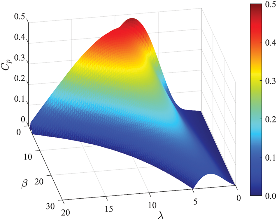
Figure 2: Changes in wind energy utilization coefficient

As can be seen from Fig. 2, when the pitch angle and the tip speed ratio , the wind energy utilization coefficient can reach a maximum value of 0.48. However, when the tip speed ratio remains unchanged, as the pitch angle increases, will show a downward trend, and there is an inverse relationship between the two. Since the object of this study is a direct-drive permanent magnet synchronous offshore wind power generation system, the offshore wind turbine and the generator adopt a direct drive mode without the aid of a speed increase gearbox. Under the premise of ignoring the influence of rigid body torque, the mechanical angular velocity of the offshore wind turbine and the generator is equal, then the kinematic equation of the offshore wind turbine is expressed as Eq. (5):

(5)

In the equation, is the equivalent moment of inertia; is the damping coefficient; is the electromagnetic torque of the generator.

2.1.2 Generator Mathematical Model

The offshore wind power generation system in this study adopts the widely used permanent magnet synchronous generator (PMSG). The three-phase part of this motor has a strong coupling property, and the relationship between its variables also shows significant nonlinearity, which makes it difficult to directly control the motor effectively. In order to overcome this problem, the common practice is to first transform the complex original model into a simpler equivalent model through coordinate transformation, and then carry out subsequent research work on this basis, which helps to simplify the design and implementation of the control strategy. In order to simplify the model establishment and analysis process, the three-phase PMSG is usually regarded as an ideal motor, including the following idealized assumptions: ignoring the effects of magnetic circuit saturation, eddy current loss and hysteresis loss, and considering the magnetic permeability of the core part as a constant. The rotor winding is symmetrical on the longitudinal and transverse axes, respectively; the stator winding is completely consistent in structure, and its air gap magnetomotive force conforms to the sinusoidal distribution law in space. The rotor surface is smooth and has no bumps, and the influence of high-order harmonics is ignored; the permanent magnet flux remains constant and is a constant value. Under the above-idealized assumptions, the voltage equations of PMSG in the natural coordinate system can be derived as Eq. (6):

(6)

In the formula, , , and represent the phase voltages in the three-phase stator windings; , , and represent the phase currents in the three-phase stator windings; is the equivalent resistance of the stator windings; , , and represent the flux linkages in the three-phase stator windings. To simplify the analysis process, the original equation can be transformed into the synchronously rotating d-q reference coordinate system according to Clark and Park transformation. In the new coordinate system, the d-axis is aligned with the direction of the rotor permanent magnet flux, while the q-axis is ahead of the d-axis by a certain phase angle. After this coordinate transformation, the original voltage equation in the d-q synchronously rotating coordinate system becomes Eq. (7):

(7)

The magnetic flux equation in the d-q axis coordinate system is Eq. (8):

(8)

Substituting Eq. (7) into Eq. (8) further decouples the voltage equation to obtain Eq. (9):

(9)

In the above formula, and are the d-axis and q-axis voltages of the generator stator, respectively; and are the d-axis and q-axis currents of the generator stator; and are the d-axis and q-axis flux linkages of the generator stator; and are the d-axis and q-axis inductances of the generator stator; is the electrical angular velocity of the generator rotor; and is the rotor permanent magnet flux linkage. The electromagnetic torque equation of the permanent magnet synchronous motor can be expressed as Eq. (10):

(10)

where is the number of pole pairs.

2.1.3 Analysis of Offshore Wind Turbine Operation Characteristics

Since the direct-drive permanent magnet synchronous offshore wind power generation system in this study belongs to a variable-speed offshore wind power generation system, the variable-speed offshore wind power generation system can be divided into four different areas according to different wind speeds, as shown in Fig. 3.

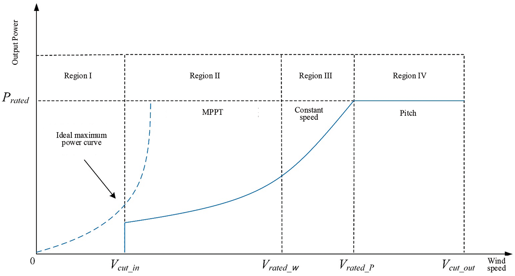
Figure 3: Schematic diagram of the operating area of the variable speed offshore wind power generation system

The first area is the start-up preparation interval of the offshore wind power generation system. At this time, the generator set has not yet been connected to the grid. The offshore wind power generation system mainly completes the preparation work for grid connection and startup, and there is no need to implement the power control strategy for the time being. The second area is the constant wind energy utilization coefficient interval. After the wind speed reaches the starting wind speed, the offshore wind rotor accelerates to the mechanical angular velocity at which the generator is put into operation. After that, by adjusting the mechanical angular velocity of the generator, the wind energy utilization coefficient continues to rise to the maximum value, and the system operates best at this time. The control strategy focuses on maintaining the mechanical angular velocity of the offshore wind rotor near the optimal value to achieve maximum wind energy capture. The third area is the constant mechanical angular velocity interval. As the wind speed increases, the mechanical angular velocity of the offshore wind turbine will continue to increase until it reaches the maximum allowable limit. To prevent damage, the control system will lock the mechanical angular velocity unchanged. Although the wind energy utilization coefficient decreases, the output power of the whole unit will still increase due to the increase in wind speed. The fourth area is the constant power interval. When the generator and power converter are close to the rated power limit, it is necessary to ensure that the system output power is maintained below the limit value. When the wind speed increases, the power coefficient will be rapidly reduced by adjusting the pitch angle, thereby locking the output power at the rated value and achieving constant power output.

Since in actual scenarios, most offshore wind power generation systems operate in the second area, the maximum power point tracking control algorithm in this area will directly affect the power generation efficiency of the entire offshore wind power generation system. In order to better study and improve the maximum power point tracking control algorithm, an offshore wind turbine simulation model was established using MATLAB/Simulink to study the operating characteristics of offshore wind turbines at different wind speeds. The simulation model is shown in Fig. 4.

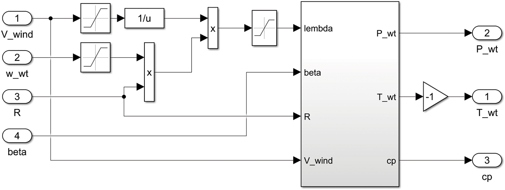
Figure 4: Offshore wind turbine simulation model

When the offshore wind turbine is simulated, the blade radius is set to 8 m, the air density is 1.225 kg/m3, and the blade pitch angle is 0°. For the wind speed , five working conditions of 8, 9, 10, 11 and 12 m/s are set, respectively, and a signal disturbance with a linear slope of 1 is applied to the mechanical angular velocity of the offshore wind turbine. Based on the above simulation setting conditions, the functional relationship curve between the wind energy utilization coefficient and the mechanical angular velocity of the offshore wind turbine, as well as the functional relationship curve between the output power of the offshore wind turbine and the mechanical angular velocity can be obtained through numerical simulation calculation, and these curves are shown in Fig. 5, respectively.

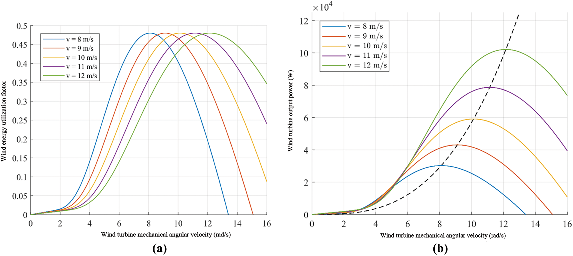
Figure 5: Offshore wind turbine output characteristic curves at different wind speeds. (a) Wind energy utilization coefficient at different wind speeds. (b) Offshore wind turbine output power at different wind speeds

It can be analyzed from Fig. 5a that under a specific blade pitch angle setting, for different wind speed conditions, the maximum value of the wind energy utilization coefficient curve is 0.48. However, under different wind speeds, the optimal mechanical angular velocity of the offshore wind turbine will be different, and the optimal mechanical angular velocity will increase with the increase of wind speed. It can be analyzed from Fig. 5b that under the condition that the mechanical angular velocity of the offshore wind turbine remains unchanged, the output power of the offshore wind turbine will show an increasing trend with the increase of wind speed. However, for a certain wind speed condition, there is an optimal mechanical angular velocity that makes the output power reach the maximum value, which is consistent with the result shown in Fig. 5a.

2.1.4 Control Framework of AC/DC Converter for Offshore Wind Power Generation System

The AC/DC converter on the machine side of the offshore wind power generation system adopts a two-level three-phase voltage-type PWM converter, and its circuit is shown in Fig. 6, where are IGBT switch tubes.

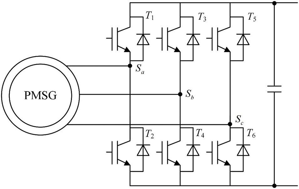
Figure 6: Schematic diagram of the structure of a two-level three-phase voltage-source PWM converter

The circuit can construct eight different logical switch states through eight combinations of switch signals Sa, Sb and Sc (000, 100, 010, 001, 011, 101, 110, 111). In these combinations, “1” represents that the upper part of the corresponding bridge arm is turned on, while “0” represents that the lower part of the corresponding bridge arm is turned on. By flexibly designing the switching sequence and switching mode of these eight logical switch states, the control system can accurately adjust the stator output voltage of the generator, thereby effectively regulating the stator current and finally optimizing the mechanical angular velocity of the generator rotor. In this process, the conversion circuit can also convert the alternating current output by the generator into direct current. In order to convert the reference voltage into a switching signal, the space vector pulse width modulation (SVPWM) technology is usually used. The main process of the algorithm is as follows: First, the reference voltage in the two-phase stationary coordinate system is converted into the corresponding amplitude and spatial displacement angle using the polar coordinate method. Next, the sector where the reference voltage is located is determined based on the calculated spatial displacement angle, and the reference voltage amplitude is used to calculate the working time of the voltage vector. Then, the working time is compared with the triangular carrier signal to generate an equivalent switching signal. Finally, the actual switching signal can be obtained based on the known sector and the equivalent switching signal, so that the actual value of the stator voltage is the same as the reference voltage.

The reference voltage can be obtained through the maximum power point tracking control algorithm. The maximum power point tracking control algorithm of this study adopts the magnetic field oriented vector control strategy framework. The control strategy is divided into outer loop and inner loop control. The reference variable of the outer loop is the optimal mechanical angular velocity, the optimal tip speed ratio or the optimal power, etc. The inner loop is the current loop, which adopts the zero d-axis current (Zero d-axis Current, ZDC) control method. It can be seen from Eq. (10) that under the control strategy of , the electromagnetic torque of the generator is only related to the q-axis current isq, which greatly simplifies the control of the electromagnetic torque. It can be seen from Eq. (9) that there is a coupling relationship between the voltage and current on the d and q axes. In order to eliminate the coupling term, the feedforward decoupling is introduced to obtain Eq. (11):

(11)

In the formula, and are the parameters of the current inner loop PI controller; and are the reference currents of the stator d and q axes respectively. Substituting Eq. (11) into Eq. (9), the decoupled current equation can be obtained as Eq. (12):

(12)

It can be seen from the common Eq. (12) that after decoupling, the change of is only related to itself and has nothing to do with . Similarly, the change of is only related to itself. As a result, the control system can independently control the d-axis and q-axis currents, thereby significantly improving the control speed and ensuring efficient and stable operation of the system. Based on this, the overall control framework based on the machine-side converter is shown in Fig. 7. The core of the control framework is the outer loop of the MPPT control algorithm. The input variable is the error between the actual control parameter M and the given target value , which will vary depending on the specific selected MPPT algorithm. The workflow of the overall control framework is summarized as follows: First, the d-axis reference current is given as 0, and the MPPT control algorithm calculates the reference value of the inner loop q-axis current based on the deviation between M and . Then, after the d- and q-axis reference currents are decoupled from the inner loop, dynamic voltage regulation components and are generated. Then, through the 2 r to 2 s coordinate transformation, the above-mentioned regulation components are converted into voltage control instructions and in the two-phase stationary coordinate system. Finally, based on the SVPWM waveform modulation technology, the switching signals , and that drive each IGBT to open and close are generated according to the control instructions.

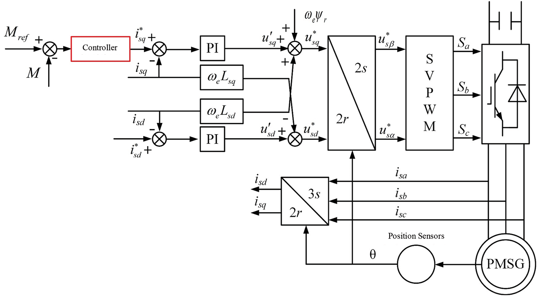
Figure 7: Control framework diagram based on machine-side converter

2.2 Research on MPPT Control Method Based on TSR and SMC Algorithm

2.2.1 MPPT Control Principle of Offshore Wind Power Generation

From the analysis in Chapter 2, it can be seen that under the setting of a given pitch angle, there is only one maximum output power point for offshore wind turbines under different wind speed conditions, that is, there is only one optimal mechanical angular velocity. When it is lower than the optimal mechanical angular velocity, the output power of the offshore wind turbine will increase with the increase of the mechanical angular velocity; but after exceeding the optimal point, the power output will begin to decrease. Therefore, if the corresponding optimal mechanical angular velocity can be quickly locked according to the change of wind speed in time, and the mechanical angular velocity of the wind turbine can be adjusted to this value, the system can achieve maximum power output under changing wind speed. The MPPT control principle of offshore wind power generation is shown in Fig. 8.

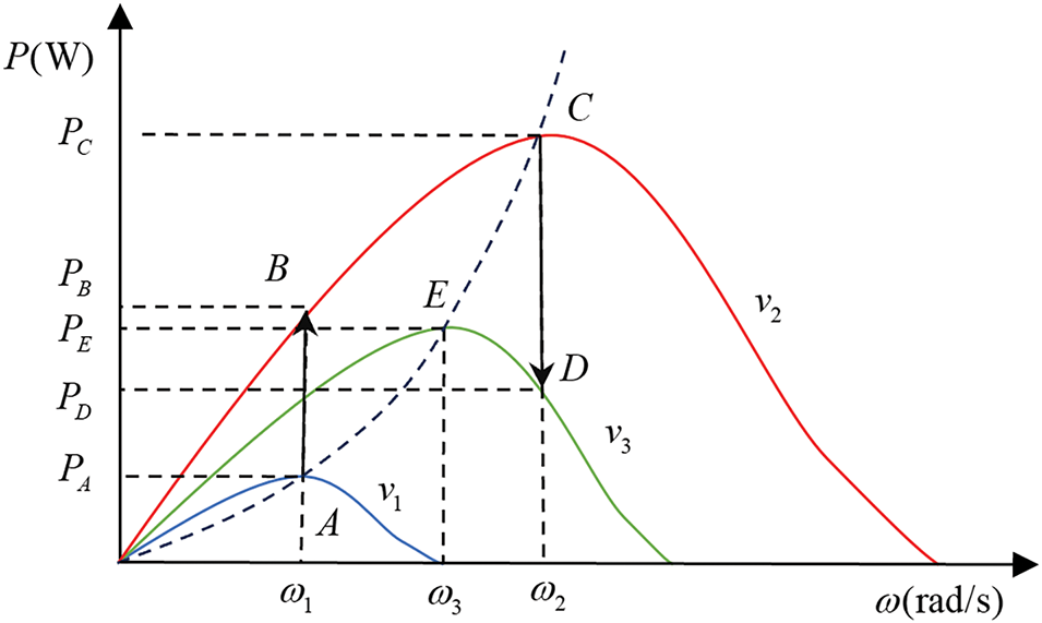
Figure 8: MPPT control principle diagram of offshore wind power generation

When the current wind speed is , the offshore wind turbine generator set operates normally at point of the maximum mechanical power curve, and the optimal mechanical angular velocity at wind speed is . At a certain moment, the wind speed changes to , that is, the wind speed increases, and the mechanical power captured by the offshore wind rotor will increase, that is, the output power of the offshore wind rotor will increase to , so it is necessary to quickly adjust the mechanical angular velocity to through the maximum power point tracking control method. When the output power of the offshore wind rotor reaches the intersection point of the offshore wind rotor power curve and the maximum power curve, the mechanical angular velocity stabilizes at the optimal mechanical angular velocity at wind speed , the electromagnetic torque and the offshore wind torque are equal, the power enters balance again, and the maximum power output of the generator is . When the wind speed suddenly drops from to , the mechanical power captured by the offshore wind rotor will drop to . At this time, it is necessary to quickly drop the mechanical angular velocity of the offshore wind rotor from to , so that the output power of the generator can track the maximum power at the wind speed .

2.2.2 Tip Speed Ratio Method and Principle of Sliding Mode Control Algorithm

From the above analysis, it can be seen that when the pitch angle is 0, if the tip speed ratio can be kept at the optimal value of 8.1, then the maximum wind energy utilization coefficient is 0.48. Therefore, maintaining the tip speed ratio at the optimal value is to ensure that the wind energy utilization coefficient is at the optimal value, and the optimal tip speed ratio λ_opt can be achieved through the optimal mechanical angular velocity ω_(wt_opt), which is equivalent to a variant of the tip speed ratio method (Tip Speed Ratio, TSR). If the mechanical angular velocity of the offshore wind turbine can be kept at this optimal mechanical angular velocity, the output power of the offshore wind turbine will be optimal regardless of the wind speed conditions, thereby achieving the goal of the offshore wind turbine to track the maximum power point. The control logic block diagram of the tip speed ratio method is shown in Fig. 9.

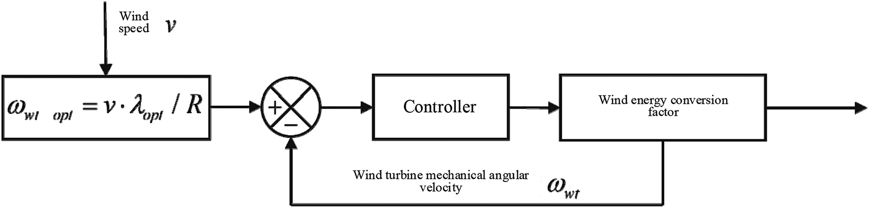
Figure 9: Control logic block diagram of the tip speed ratio method

With the advancement of sensor technology, this method has the advantages of high accuracy, simple implementation, and fast speed compared with the hill climbing search method, power signal feedback method, and optimal torque method. The tracking effect of this method is not only affected by the wind speed measurement accuracy but also by the performance of the controller. Therefore, if you want to improve the tracking effect of this method, you must study the controller. Among many control algorithms, the sliding mode control algorithm (SMC) has a good application prospect for offshore wind power generation systems in random wind speed environments due to its strong anti-interference and fast response characteristics. In the sliding mode motion control theory, the system state space is divided into three regions by a hypersurface: the region where the switching surface is located, and the two regions of and , as shown in Fig. 10. The performance of the motion state point on the switching surface varies according to its trajectory, and can be mainly divided into three situations: first, the starting motion point, as shown in the trajectory of point , initially approaches the switching surface, and when it reaches the switching surface, it moves away from the two areas; second, the ending motion point, as shown in the trajectory of point , the motion trajectory gradually approaches and eventually tends to the switching surface; third, the normal motion point, as shown in the trajectory of point in the figure, gradually approaches the switching surface and eventually crosses and continues to move. The starting motion point and the normal motion point have no meaning for the dynamic process of the system, but the ending motion point can significantly change the robustness of the controlled object under this control mode. Specifically, when the motion state trajectory gradually approaches a switching surface area formed by the termination point, it will be constrained by the switching function and attracted to move in this area. The switching surface area that meets the above conditions is defined as the “sliding mode area”, and the motion process inside it is called “sliding mode motion”.

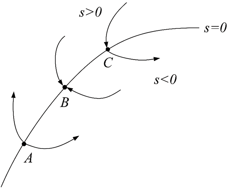
Figure 10: Schematic diagram of sliding mode control theory

The sliding mode control method is as follows, considering the nonlinear system as Eq. (13):

(13)

In the formula, refers to the state variable of the system; represents the control input applied to the system; and are functions related to the system; represents the total disturbance affecting the system. For a system that needs to implement sliding mode control, the first step is to select a suitable sliding mode switching surface . Then, based on the selected switching surface, through mathematical solution, the control function expression of the sliding mode controller can be finally derived as Eq. (14):

(14)

When the system state trajectory falls on the sliding surface, the corresponding . In order to construct an effective sliding mode control, three basic criteria need to be implemented simultaneously: existence criterion, reachability criterion and stability criterion. The existence criterion means that the system must have a sliding mode, that is, satisfy the following inequality relationship as shown in (15):

(15)

The reachability criterion means that any state point outside the sliding surface can converge to the sliding surface within a finite time, which can be expressed as (16):

(16)

From Eqs. (15) and (16), it can be seen that there is an inherent coupling relationship between the existence condition of the sliding mode and the reachability condition, that is, when , the system can meet the existence requirement of the sliding mode and ensure that the state trajectory finally converges to the sliding surface. The realization of this inequality relationship is one of the basic requirements to be followed in building a sliding mode controller. The stability condition means that when the Lyapunov function of the state point near the sliding surface is positive definite and its derivative is negative definite, the state point can remain stable near the sliding surface, and the entire system will also maintain stable operation. The mathematical expression is Eq. (17):

(17)

The motion trajectory of sliding mode control can be summarized into two typical stages. The first is the normal motion mode stage, in which the system trajectory points are mainly distributed outside the switching surface , with occasional crossing movements. The second is the sliding mode stage along the switching surface, in which the system trajectory points will completely slide in the sliding mode region on the switching surface. The dynamic quality level of these two motion modes directly determines the performance of the entire sliding mode control. Since the quality of the motion process cannot be fully optimized through a single design, the performance level of the two motion stages must be improved separately. For this reason, the design process of the sliding mode controller is generally divided into two steps: the first is the design of the switching surface, so that the system can converge to the target control point after entering the sliding mode motion and has good dynamic response quality; the second is the design of the switching control item to ensure that the system trajectory can reach the switching surface, thereby performing sliding mode motion along the switching surface.

2.2.3 MPPT Control Algorithm Based on GFISMC Algorithm

From the above research, it can be seen that after adopting rotor flux oriented control and voltage feedforward decoupling, the control strategy on the machine side is divided into an outer loop and an inner loop. The inner loop generally adopts a PI controller, while the outer loop is the focus of this study. The reference mechanical angular velocity of the outer loop is determined by TSR. In order to improve the tracking speed, this study adopts a global fast integral sliding mode control (GFISMC) in the controller of the outer loop. The sliding surface adopts a new type of fast integral sliding surface, and the approach part adopts a new type of fuzzy fast switching control item, which can make the mechanical angular velocity globally and quickly track to the optimal mechanical angular velocity.

(1) Fast integral sliding surface

The state variable of the machine side converter system is defined as Eq. (18):

(18)

Substituting Eq. (18) and its derivative into Eq. (13), we obtain Eq. (19):

(19)

After rearranging, we can get the state Eq. (20):

(20)

here, , , , .

is the total interference term in the dynamic equation composed of uncertain parameters and external interference, is the total interference term under the state equation, and . is the compensation coefficient used to compensate for the interference term. In order to ensure that the state variables converge quickly within a finite time and improve the robustness of the system, a fast integral sliding surface is used as Eq. (21):

(21)

here, , .

If the initial value of the integral on the sliding surface is known, then is zero at the initial moment, which means that the initial state of the system is on the sliding surface, thereby enhancing the system’s ability to resist interference. The transient process of this method is closely related to the initial value of the integral. In order to obtain the initial value of the integral and ensure the smoothness of the target speed, a first-order low-pass filter can be used to temporarily process the target speed when a sudden change signal is detected. Its description form is Eq. (22):

(22)

here, . Where is the cutoff frequency. The initial target value after processing is 0, that is, the initial reference mechanical angular velocity is 0, so it can be known that the initial value of the integral is 0, and the new fast integral sliding surface can be obtained as Eq. (23):

(23)

When the system enters the sliding mode, , which is Eq. (24):

(24)

The design goal of the fast integral sliding surface is to make the system trajectory continue to run on the switching surface. However, due to the influence of external disturbances and parameter uncertainty, the motion trajectory of the actual system often presents a sawtooth motion along the switching surface, and the system error state quantity may be an arbitrary value. As shown in Eq. (24), when the error state quantity is far away from the equilibrium point, the term plays a dominant role; and when the error state variable is close to the equilibrium point, the term plays a dominant role. Therefore, compared with the traditional sliding surface , the proposed sliding surface has better rapid convergence performance. Different from the traditional sliding surface , for any initial error state, the proposed sliding surface can make the error state quantity converge to 0 in a finite time. Assuming , Eq. (24) can be expressed as Eq. (25):

(25)

By dividing both sides of the equation by , it can be transformed into Eq. (26):

(26)

Define a new variable , so , substitute into Eq. (26) and simplify to get Eq. (27):

(27)

Solving Eq. (27), we can get the general solution to Eq. (28):

(28)

For the initial condition x(0) = x0, the general solution can be transformed into Eq. (29):

(29)

here, , .

Based on this, the time T required for the system to reach stability is Eq. (30):

(30)

From Eq. (30), it can be seen that the maximum value of the stabilization time can be expressed as Eq. (31):

(31)

Eq. (31) shows that the designed sliding surface ensures that the system error state variable returns to zero within a finite time, and this upper bound of the stable time does not depend on the size of the initial error state variable.

(2) Fuzzy fast switching control term

Taking into account the influence of external disturbances and uncertain parameters, and in order to ensure the high robustness of the system and that the system motion trajectory always moves toward the switching surface, this study uses the design method of equivalent sliding mode control to design the control law. The equivalent sliding mode control is divided into two parts: one is the switching control term in the approaching motion stage, and the other is the equivalent control term on the sliding surface. The equivalent control term is determined by the sliding surface designed above, and the switching control term is the focus of this section. Without considering the disturbance, it is assumed that the sliding mode control law that has been obtained makes the sliding surface a dead point and satisfies . Combining Eqs. (30) and (31), the equivalent control term can be obtained as Eq. (32):

(32)

In order to ensure that the system can reach the sliding surface when considering interference, a new switching control term is adopted as Eq. (33):

(33)

In the formula, , , are positive odd number to ensure that the system convergence conditions are met.

It can be seen from Eq. (33) that when the system is far away from the sliding surface, the term plays a major role; when the system approaches the sliding surface, the term plays a major role. Therefore, in the approach motion stage, the proposed switching control term can enable the system to quickly reach the sliding surface. It can be seen from Eq. (32) that the equivalent control term is essentially continuous, achieving a smooth transition and greatly reducing control jitter. It can be seen from Eq. (33) that during the switching process, the term and the term are continuous, while the switching function of the compensation term is not continuous, which may cause high-frequency jitter. In order to reduce jitter, this study uses the function instead of the function, and Eq. (34) is obtained:

(34)

When is 0.1 and is different, the function is shown in Fig. 11. As shown in Fig. 11, when is closer to 0, the function is closer to the function, and the overall smoothness is better, and the convergence speed will be faster. In addition, because of the existence of the function, the sliding mode control will have stronger robustness in the case of external disturbances.

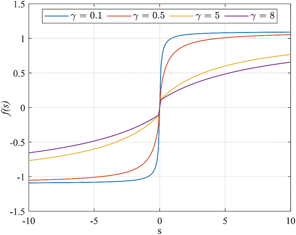
Figure 11: Graph of the function

Combining Eqs. (33) and (34), the control law of the global fast integral sliding mode can be obtained as Eq. (35):

(35)

In specific application scenarios, the disturbance has a time-varying characteristic. If the setting value of the disturbance compensation is too single, it will face different challenges: in the low-speed link, the actual disturbance may be much smaller than , which is easy to cause severe vibration. In the high-speed link, the disturbance d may far exceed , causing the system to fail to meet the Lyapunov stability condition, thereby affecting the stability of the system. Therefore, the dynamic adaptive adjustment of can be achieved by applying fuzzy control technology to enhance the system’s resistance to disturbances. In this study, and are used as the input variables of the fuzzy controller, and is used as the output variable. The domain of the input variable is defined as [−10, 10], which is divided into five intervals {NB, NS, ZO, PS, PB}; the domain of the output variable is set to [0, 6], which is also divided into five intervals {SS, S, M, B, BB}. The fuzzy rules are shown in Table 1. When the values of and are large, it means that the disturbance to the system increases, so the compensation gain needs to be increased accordingly. On the contrary, the compensation gain needs to be reduced. In particular, when , it means that the interference is too large and the compensation gain needs to be increased to ensure the convergence of the system. When , the system is in a convergence state, and appropriately reducing the compensation gain can reduce the jitter phenomenon.

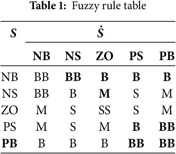
The membership function can be used to fuzzify the precise numerical value. In this study, a triangular membership function is selected, and the centroid method is used for defuzzification. The fuzzy membership function is shown in Fig. 12.

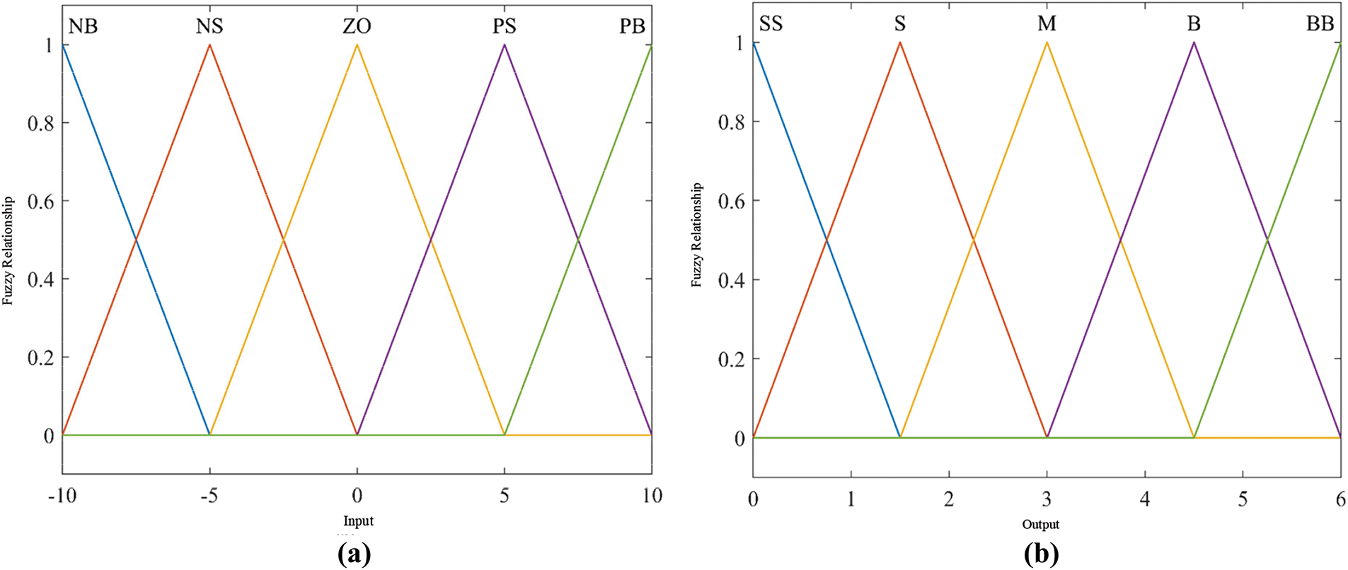
Figure 12: Membership relationship based on triangle type. (a) Membership relationship of input variables. (b) Membership relationship of output variables

2.2.4 Proof of Stability and Effectiveness of GFISMC Algorithm

Define the Lyapunov function as Eq. (36):

(36)

Taking the derivative of , we get Eq. (37):

(37)

It can be seen that when , is globally valid. Therefore, the fuzzy compensation coefficient controller can be used to achieve , thereby ensuring the asymptotic stability of the system in a global sense. In order to quickly verify the stability and effectiveness of the algorithm, a first-order system was built in MATLAB/Simulink for verification, with parameters , , , and the tracking signal . The sliding mode parameters are , , , , , , , , . Fig. 13 is the tracking effect diagram.

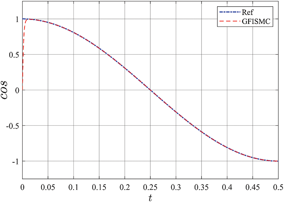
Figure 13: Tracking effect verification diagram

As can be seen from Fig. 13, the GFISMC algorithm smoothly tracks the cosine signal at around 0.01 s, and can always track the reference signal under interference conditions, indicating that the GFISMC algorithm not only has fast tracking but also has strong anti-interference ability.

2.3 MPPT Simulation Analysis of Offshore Wind Power Generation System

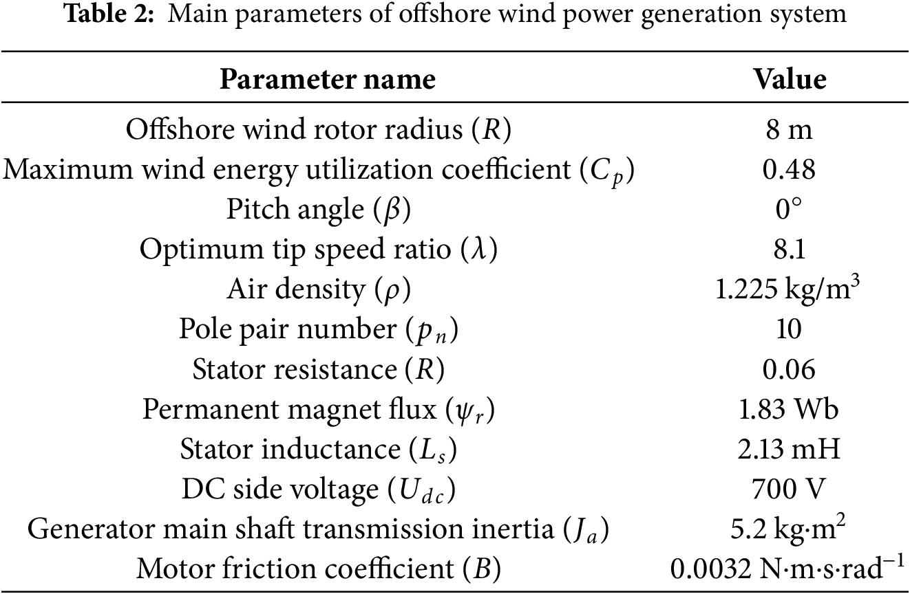
In order to verify the effect of the proposed algorithm in the offshore wind power generation system, this study established an offshore wind power generation system model based on permanent magnet synchronous motor with the help of MATLAB/Simulink. The model includes permanent magnet synchronous motor and AC/DC converter, as shown in Fig. 14. Considering that the control essence of the algorithm is to control the mechanical angular velocity of the generator to quickly reach the optimal mechanical angular velocity, in order to quickly verify the tracking effect of the proposed algorithm, the huge inertia of the offshore wind wheel is ignored in the model. The key parameters of the offshore wind power generation system are listed in Table 2.

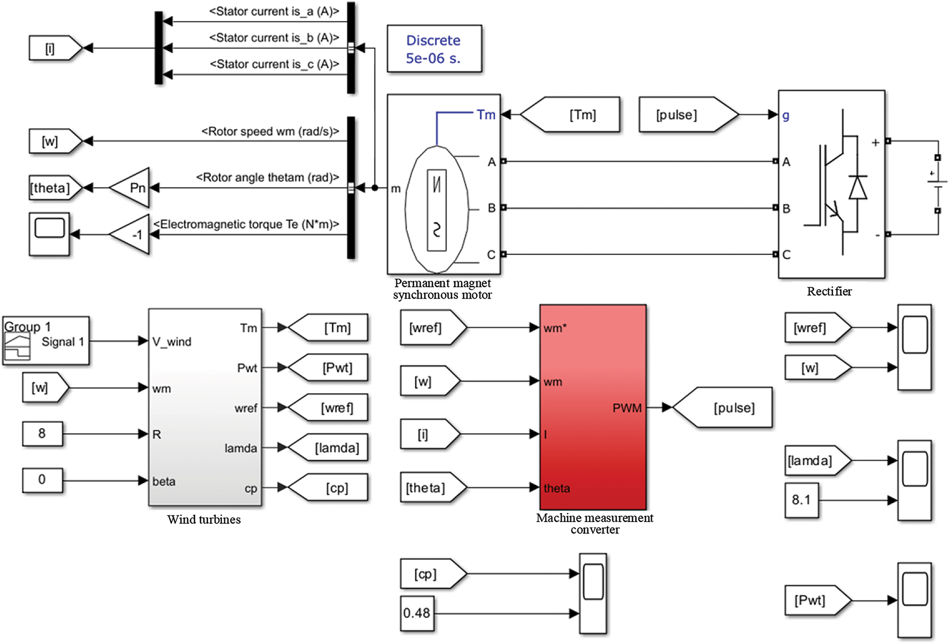
Figure 14: Offshore wind power generation system model

Based on the above conditions, simulation verification was carried out under step wind speed and random wind speed, and GFISMC, SMC and PI were compared. The parameters of the GFISMC algorithm are: , , , , , , , , , , .

2.3.1 MPPT Simulation Analysis under Step Wind Speed

In order to verify the effectiveness of the proposed control algorithm, a corresponding test is performed using step wind speed. The simulation time is set to 0.9 s. The wind speed change is shown in Fig. 15. The wind speed increase increases with time. At 0 s, the wind speed is 7 m/s; at 0.3, the wind speed jumps from 7 to 9 m/s, in order to further test the performance of the algorithm; at 0.6 s, the wind speed continues to rise, and the amplitude becomes larger, which can test the stability and robustness of the control algorithm to the greatest extent.

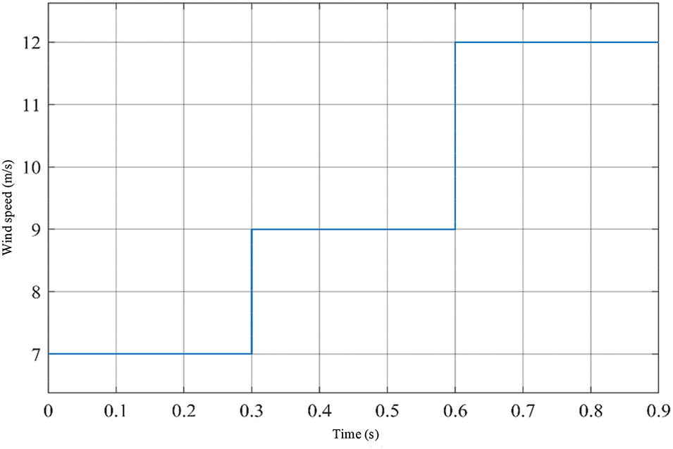
Figure 15: Step wind speed diagram

Figs. 16–19 are performance indicators of each algorithm when tracking the maximum power point. These performance indicators can reflect the specific effect of the control algorithm.

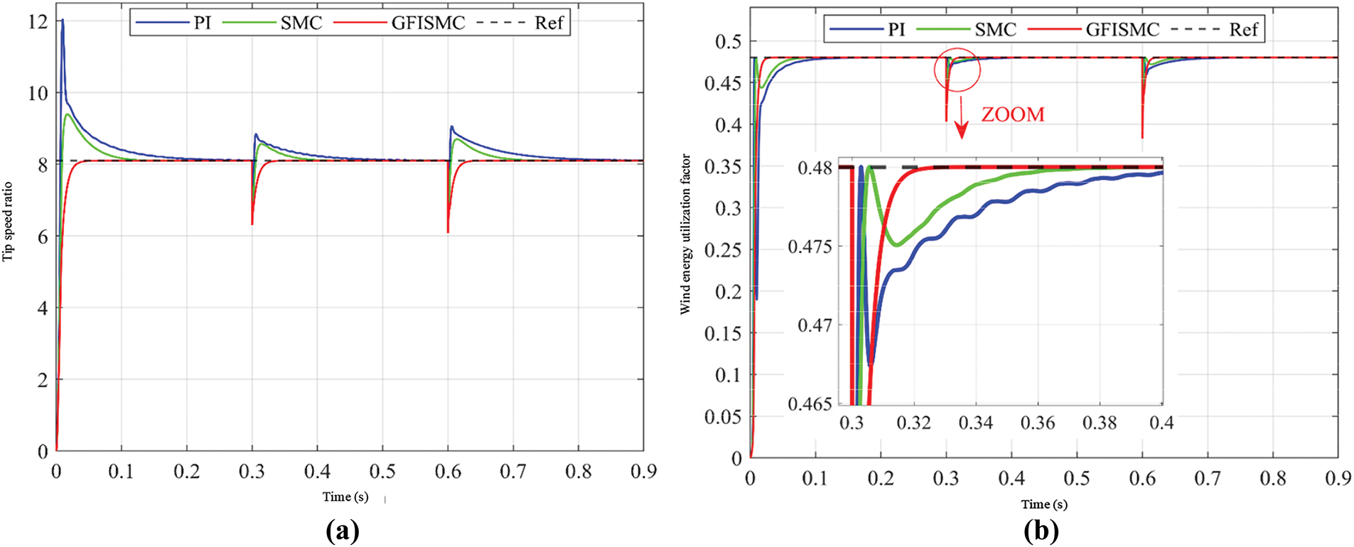
Figure 16: Tip speed ratio and wind energy utilization coefficient of offshore wind turbines under step wind speed. (a) Tip speed ratio of offshore wind turbine. (b) Wind energy utilization coefficient of offshore wind turbines

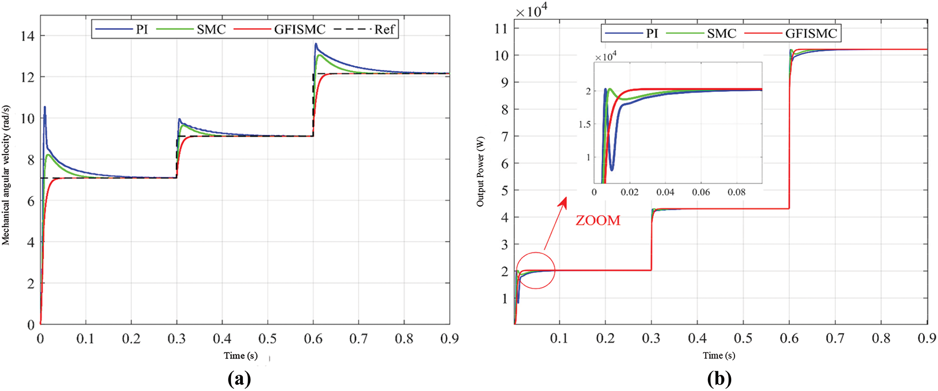
Figure 17: Mechanical angular velocity and output power of offshore wind turbines under step wind speed. (a) Mechanical angular velocity of offshore wind turbine. (b) Output power of offshore wind turbines

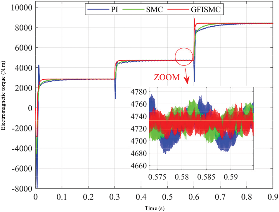
Figure 18: Generator electromagnetic torque under step wind speed

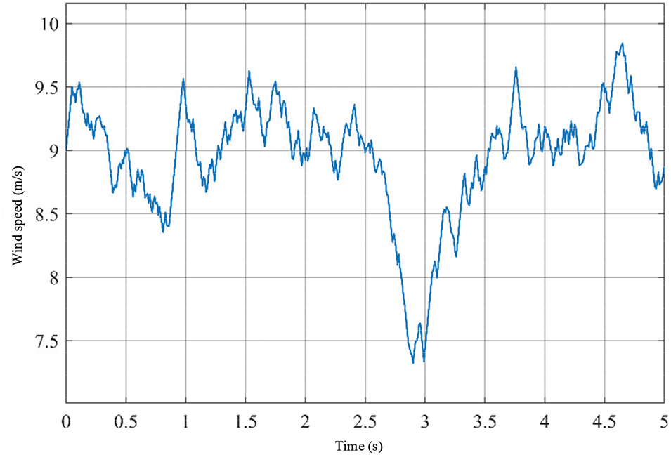
Figure 19: Random wind speed graph

Fig. 16a,b shows the response effects of the two parameters, tip speed ratio and wind energy utilization coefficient. It can be seen that in the case of a sudden change in wind speed, the GFISMC algorithm can quickly track the two optimal parameters of 8.1 and 0.48, while the SMC and PI algorithms can also track these two parameters, but the tracking amplitude is relatively large and the speed is slow. As shown in Fig. 17a, when the wind speed changes stepwise, the GFISMC algorithm proposed in this study can track the optimal mechanical angular velocity in about 0.03 s, and there is almost no overshoot, with good tracking quality. As shown in Fig. 17b, since the GFISMC algorithm can smoothly track the optimal mechanical angular velocity, the output power of the offshore wind turbine in the figure can respond quickly and has almost no fluctuations.

As shown in Fig. 18, compared with the SMC and PI algorithms, the algorithm proposed in this study not only has a fast response speed, but also causes less electromagnetic torque jitter when in steady state, which can not only reduce the generation of harmonics, but also help to improve the life of the entire power generation system equipment.

2.3.2 MPPT Simulation Analysis under Random Wind Speed

The wind speed in reality will not fluctuate greatly in the short term, but it will not always remain at a constant value, and most of them are random fluctuation signals. Therefore, in order to maximize the effect of the control algorithm under actual conditions, this section simulates and verifies the proposed algorithm under random wind speed, and the simulation time is set to 5 s. The random wind speed situation is shown in Fig. 19.

The basic wind speed of the random wind speed is 9 m/s, and the overall fluctuation is between 7.5 and 10 m/s. There is a large drop at 2.6 s, which can test the robustness of the control algorithm under random wind speed. Figs. 20–22 are the output characteristic curves of the offshore wind power generation system under random wind speed.

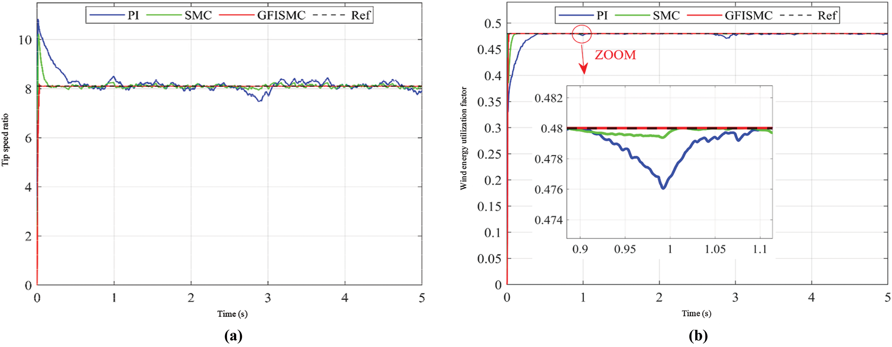
Figure 20: Tip speed ratio and wind energy utilization coefficient of offshore wind turbines under random wind speeds. (a) Tip speed ratio of offshore wind turbine. (b) Wind energy utilization coefficient of offshore wind turbines

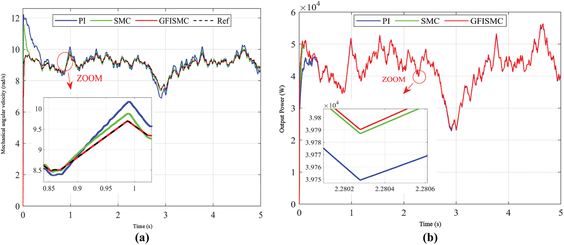
Figure 21: Mechanical angular velocity and output power of offshore wind turbines under random wind speeds. (a) Mechanical angular velocity of offshore wind turbine. (b) Output power of offshore wind turbines

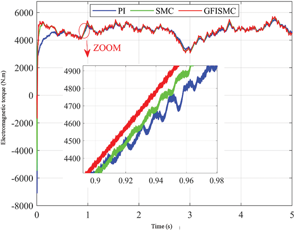
Figure 22: Generator electromagnetic torque under random wind speed

It can be seen from Fig. 20a,b that under random wind speed, the tip speed ratio and wind energy utilization coefficient of the GFISMC algorithm can be maintained at 8.1 and 0.48, indicating that the GFISMC algorithm has stronger robustness and anti-interference ability than the PI and SMC algorithms.

As shown in Fig. 21a, under random wind speed, the optimal mechanical angular velocity changes with the change of wind speed, and the mechanical angular velocity under the GFISMC algorithm can always track the optimal mechanical angular velocity, and the tracking accuracy is significantly higher than that of the SMC and PI algorithms. As shown in Fig. 21b, due to the relatively high tracking accuracy of the GFISMC algorithm, the output power of the offshore wind turbine under its control is higher than that of the SMC and PI algorithms under random wind speed.

As can be seen from Fig. 22, under random wind speed, each algorithm still has jitter during steady-state tracking, but the jitter amplitude of the GFISMC algorithm is still small, indicating that the GFISMC algorithm also has better tracking quality under random wind speed and can effectively reduce power loss.

3  MPPT Simulation Analysis of Offshore Wind-Solar Hybrid Power Generation System

The above research used independent offshore wind power generation systems and offshore photovoltaic power generation systems to verify the improved MPPT control algorithm separately. In order to further verify the feasibility and effectiveness of the improved algorithm in a complete offshore wind-solar hybrid power generation system, this section built an off-grid offshore wind-solar hybrid power generation system model in MATLAB/Simulink, and combined with Yuankuan Energy’s ModelingTech semi-physical simulation platform to carry out semi-physical verification analysis of the improved algorithm.

3.1 Analysis of the Working Mode of Offshore Wind-Solar Complementary Power Generation System

Offshore wind-solar resources often have a certain degree of complementarity on a time scale. Therefore, for off-grid microgrids, an offshore wind-solar complementary power generation system composed of an offshore wind power generation system and an offshore photovoltaic power generation system can maximize the stability of power output and improve the utilization rate of offshore wind-solar resources. The specific working conditions of the offshore wind-solar complementary power generation system are closely related to weather conditions. Theoretically, the weather conditions of the offshore wind-solar complementary system can be roughly divided into four categories: wind and sunshine, wind but no sunshine, no wind and sunshine, and no wind and no sunshine. Under different weather conditions, the offshore wind power generation module and the offshore photovoltaic power generation module in the offshore wind-solar complementary power generation system are combined or supplemented with each other, and there will be different working modes. According to the above four weather conditions, four operating modes of the offshore wind-solar complementary system can be obtained: offshore wind-solar power generation modules work together; offshore wind power generation modules work alone; offshore photovoltaic power generation modules work alone; offshore wind-solar complementary power generation modules stop working. In different working modes, according to the relationship between offshore wind power generation power , offshore photovoltaic power generation power , DC load power consumption and battery SOC, the system can be subdivided into the following working modes. The energy flow is shown in Fig. 23.

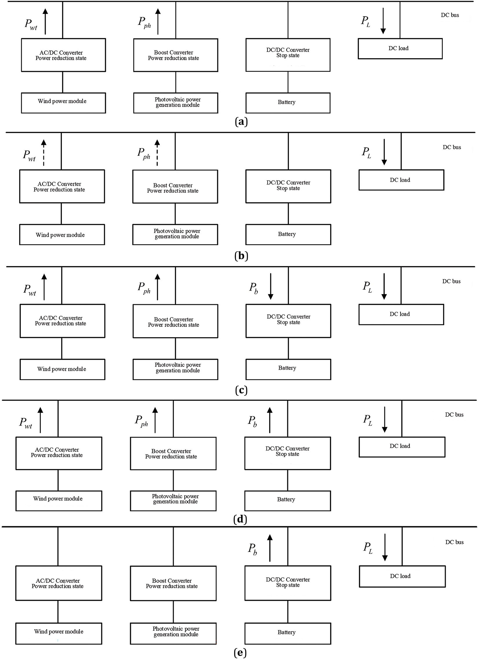
Figure 23: Energy flow diagram. (a). Mode I. (b). Mode II. (c). Mode III. (d). Mode IV. (e). Mode V

Mode 1: In this mode, the weather conditions are sunny and windy, , . At this time, in order to prevent overcharging, the battery stops working; the offshore photovoltaic power generation and offshore wind power generation modules are in a reduced power working state, and the voltage on the DC bus is stabilized by the offshore photovoltaic power generation and offshore wind power generation modules using droop control, as is shown in Fig. 23a.

Mode 2: In this mode, the weather conditions are sun without wind or sun without wind, or , . At this time, to prevent overcharging, the battery stops working; the offshore photovoltaic or offshore wind power generation module is in a reduced power working state; the voltage on the DC bus is stabilized by the offshore photovoltaic or offshore wind power generation module using constant voltage control, as is shown in Fig. 23b.

Mode 3: In this mode, the weather conditions are any one, , . At this time, the battery is in the charging state; the offshore photovoltaic power generation and offshore wind power generation modules are in the MPPT working state; the DC bus voltage is stabilized by the battery using constant voltage control, as is shown in Fig. 23c.

Mode 4: In this mode, the weather condition is any , . At this time, the battery is in the discharge working state; the offshore photovoltaic power generation and offshore wind power generation modules are in the MPPT working state; the voltage on the DC bus is stabilized by the battery using constant voltage control, as is shown in Fig. 23d.

Mode 5: In this mode, the weather condition is no wind and no sun, . The battery is in a discharge state; the offshore photovoltaic power generation and offshore wind power generation modules are not working; the voltage on the DC bus is stabilized by the battery using constant voltage control, as is shown in Fig. 23e.

It can be seen that under different weather conditions, the offshore wind-solar hybrid power generation system has five working modes. When the entire system is in mode three and mode four, the power generation module is in the MPPT state. Since the focus of this study is the MPPT control research of the offshore wind-solar hybrid power generation system, the feasibility and effectiveness of the MPPT control algorithm improved in the first two chapters will be verified in mode three and mode four.

3.2 Simulation Analysis Based on MATLAB/Simulink

In order to verify the feasibility and effectiveness of the improved MPPT control algorithm in the offshore wind-solar hybrid power generation system, an offshore wind-solar hybrid power generation system consisting of an offshore photovoltaic power generation system, a direct-drive permanent magnet offshore wind power generation system, a battery offshore energy storage system and a DC load was built using MATLAB/Simulink. The simulation model is shown in Fig. 24.

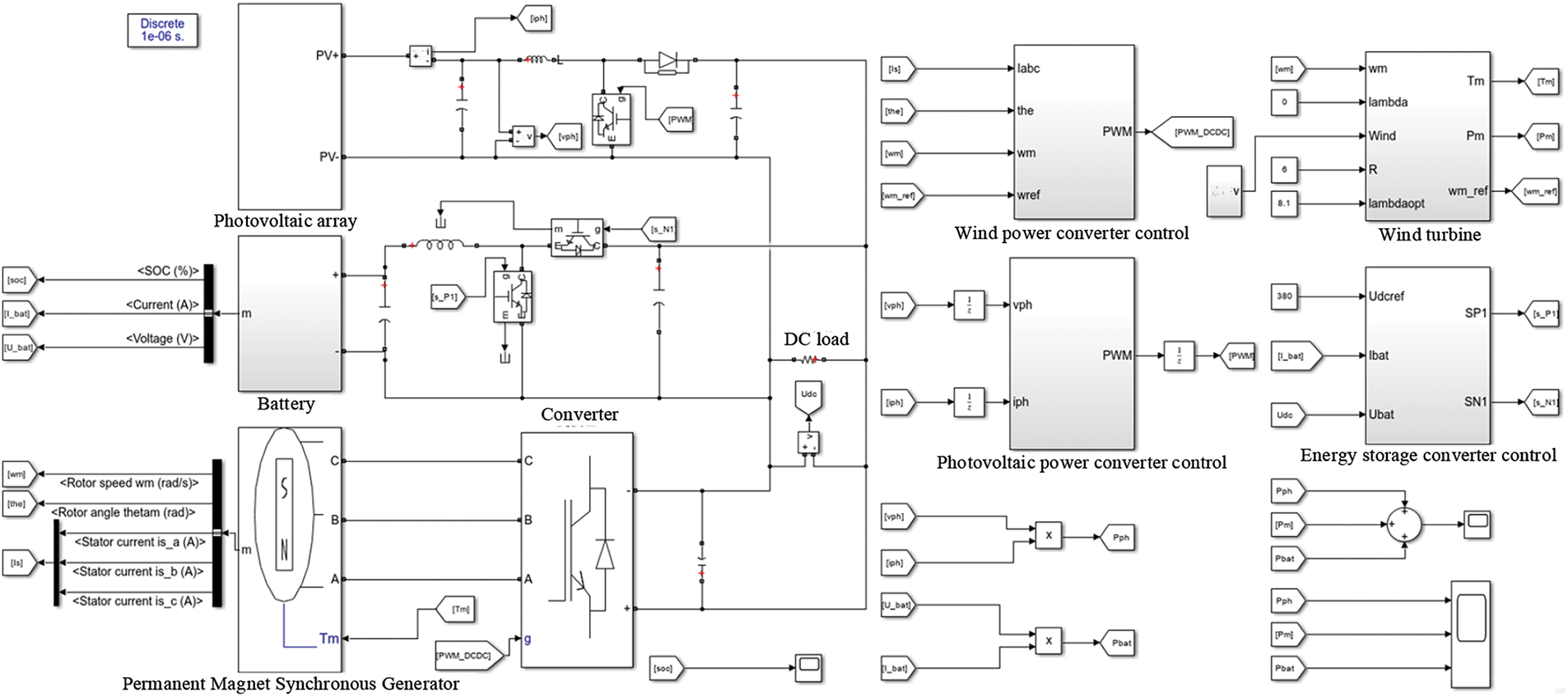
Figure 24: Offshore wind-solar hybrid power generation system model

In the offshore wind-solar hybrid power generation system, the coordinated operation of each unit power needs to be considered, and the parameters are set as follows: the DC load power is 15 kW. The rated voltage of the DC bus is 380 V; in order to facilitate the observation of the change in the state of charge, the rated voltage of the battery assembly is 235 V, the capacity is 50 Ah, and the initial SOC is 50%. The offshore wind rotor radius of the offshore wind power generation subsystem is 6 m, and the parameters of the permanent magnet synchronous generator are shown in Table 2. The offshore photovoltaic array of the offshore photovoltaic power generation subsystem is composed of 3 small offshore photovoltaic arrays in series, and each small offshore photovoltaic array is composed of 3 × 12 offshore photovoltaic cells in series and parallel. The parameters of each offshore photovoltaic cell are shown in Table 2. In addition, in order to minimize the impact of the volatility of the offshore wind power generation system and the offshore energy storage system on the maximum power point tracking of the offshore photovoltaic power generation system, this model adds a PI-based voltage control loop to the controller part of the offshore photovoltaic power generation system, but the overall control essence has not changed, except that the initial population of the UIGWO-INC algorithm is changed from the duty cycle D to the output voltage of the offshore photovoltaic array.

Based on the above simulation model, the wind speed is set as a random condition, and the light is set as a dynamic partial shading condition. Since the rapid convergence of GFISMC and UIGWO-INC has been independently verified in the previous chapters, the focus of this section is to verify the feasibility and effectiveness of these two improved algorithms running on the offshore wind-solar hybrid power generation system at the same time. Therefore, only GFISMC and UIGWO-INC are used for simulation experiments in mode three and mode four. The key parameters of the UIGWO-INC algorithm are as follows: the initial output voltage range is set to 80 to 270 V; the population size is 5, the maximum number of iterations is 8; the perturbation step size of the INC algorithm is 0.5 V. The key parameters of the GFISMC algorithm are as follows: , , , , , , , , , , . The overall simulation is divided into two stages. 0 s to 2 s is the initial stage, and the offshore wind-solar hybrid power generation system is in mode three; 2 s later is the second stage, and the offshore wind-solar hybrid power generation system is in mode four. The wind speed conditions in these two stages are both random wind speeds. As shown in Fig. 25a, the basic wind speeds in the two stages are 6 and 5 , respectively, and the overall fluctuation is between 4.5 and 7 . The temperature conditions in both stages are 25°C, and the illumination conditions are local shadows with different situations. The output characteristic curves of the overall offshore photovoltaic array under these two lighting conditions are shown in Fig. 25b. In the initial stage, the light intensity received by the three small offshore photovoltaic arrays is F1: 1000, 800 and 600 , respectively, and the maximum output power is 14,891 W. At 0.2 s, the light intensity received by the small offshore photovoltaic array is F2: 400, 550 and 200 , respectively, and the maximum output power is 5947 W.

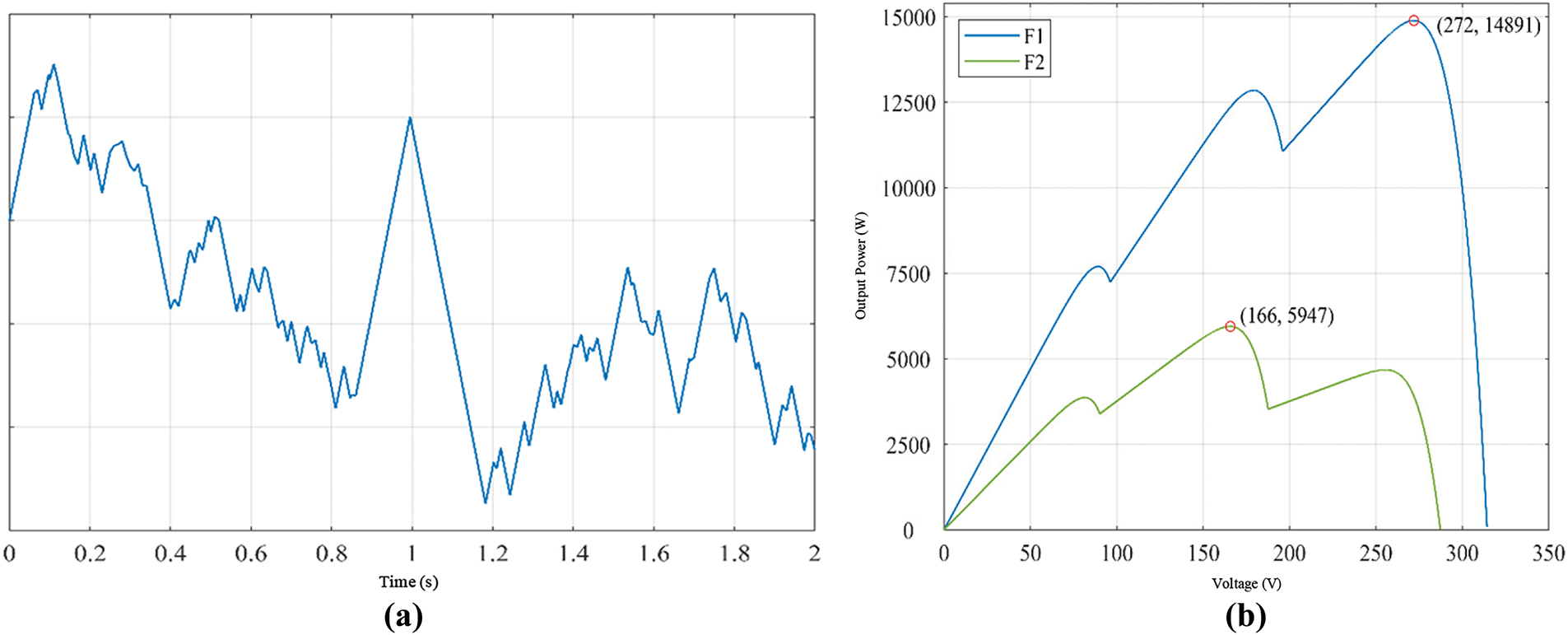
Figure 25: Random wind speed and output power characteristics of offshore photovoltaic arrays. (a) Random wind speed. (b) Output power characteristics of offshore photovoltaic arrays

The response curves in Figs. 26–28 are key indicator curves for the operation of each component, which reflect the specific effects of the improved algorithm on the offshore wind-solar complementary power generation system.

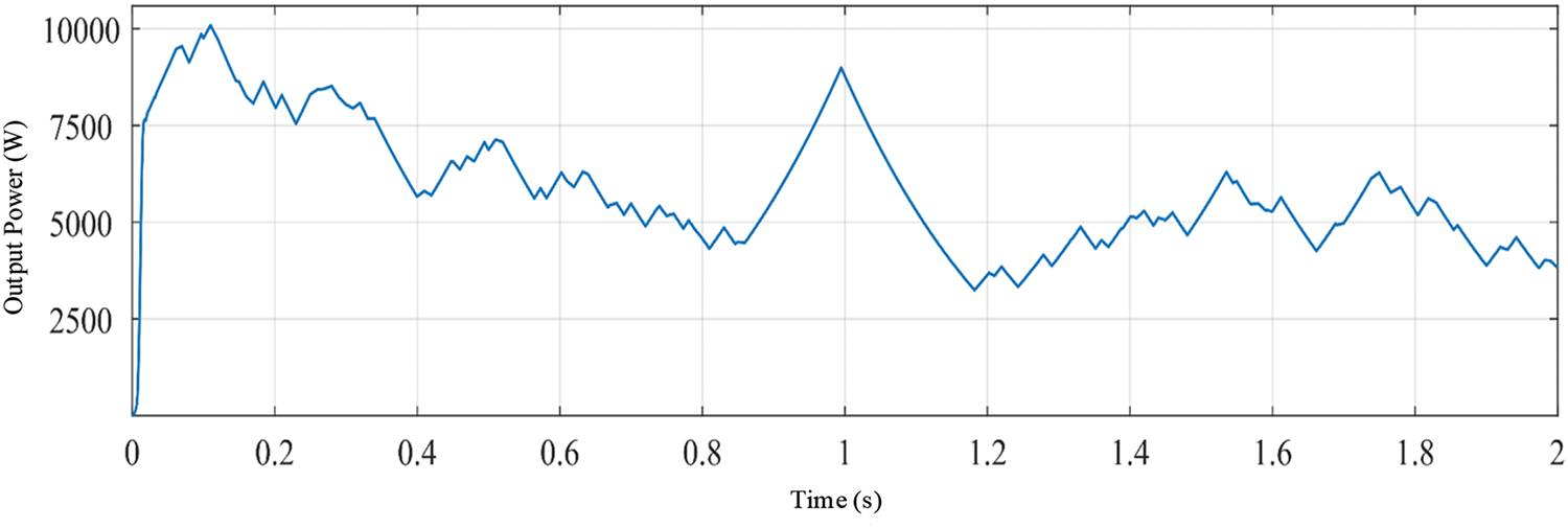
Figure 26: Offshore wind turbine output power under offshore wind and solar simulation

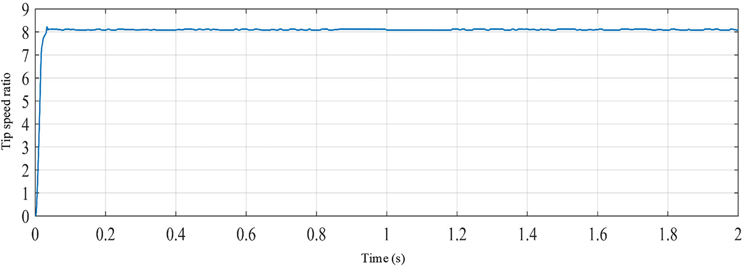
Figure 27: Tip speed ratio under light simulation

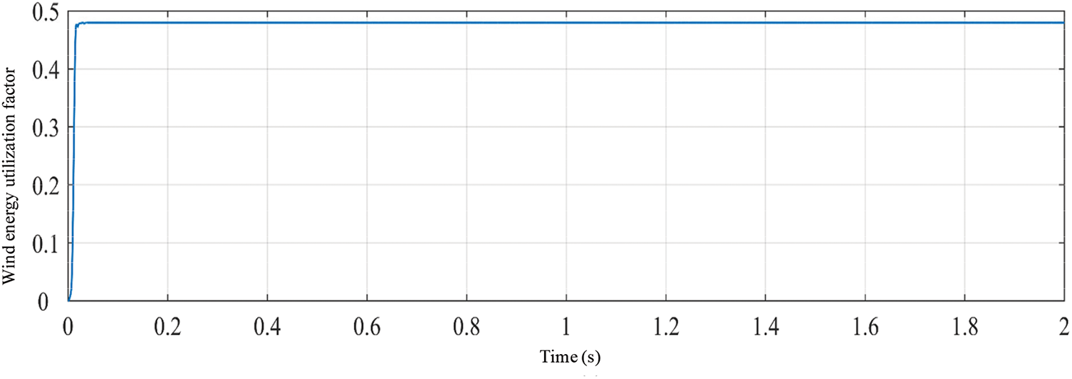
Figure 28: Wind energy utilization coefficient under light simulation

It can be seen from Figs. 26–28 that although the tip speed ratio and wind energy utilization coefficient of the offshore wind rotor under random wind speeds fluctuate, they have been stable at around 8.1 and 0.48, indicating that the output power of the offshore wind rotor in Fig. 28 has been stable at the maximum power of each random wind speed value.

As shown in Fig. 29, although the output power is affected by the voltage fluctuation on the DC bus during the tracking stage, it can quickly stabilize near the maximum power point in both the first and second stages. In the first stage, the offshore photovoltaic power generation system tracked to about 14,593 W after about 0.17 s, with a tracking accuracy of 98%. In the second stage, due to the small fluctuation of the DC bus voltage, the offshore photovoltaic power generation system tracked to about 5887 W after about 0.07 s, with a tracking accuracy of 99%.

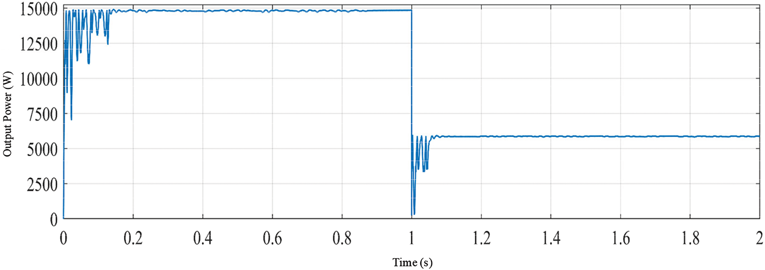
Figure 29: Offshore photovoltaic array output power under offshore wind and solar simulation

As shown in Fig. 30, when the entire power grid was first started, the offshore wind power generation and offshore photovoltaic power generation modules had not yet entered the working state, and the output power of the battery had a discharge step. Overall, the operating state of the battery changes with the changes in wind speed and light intensity, which provides a guarantee for the stability of the voltage on the DC bus.

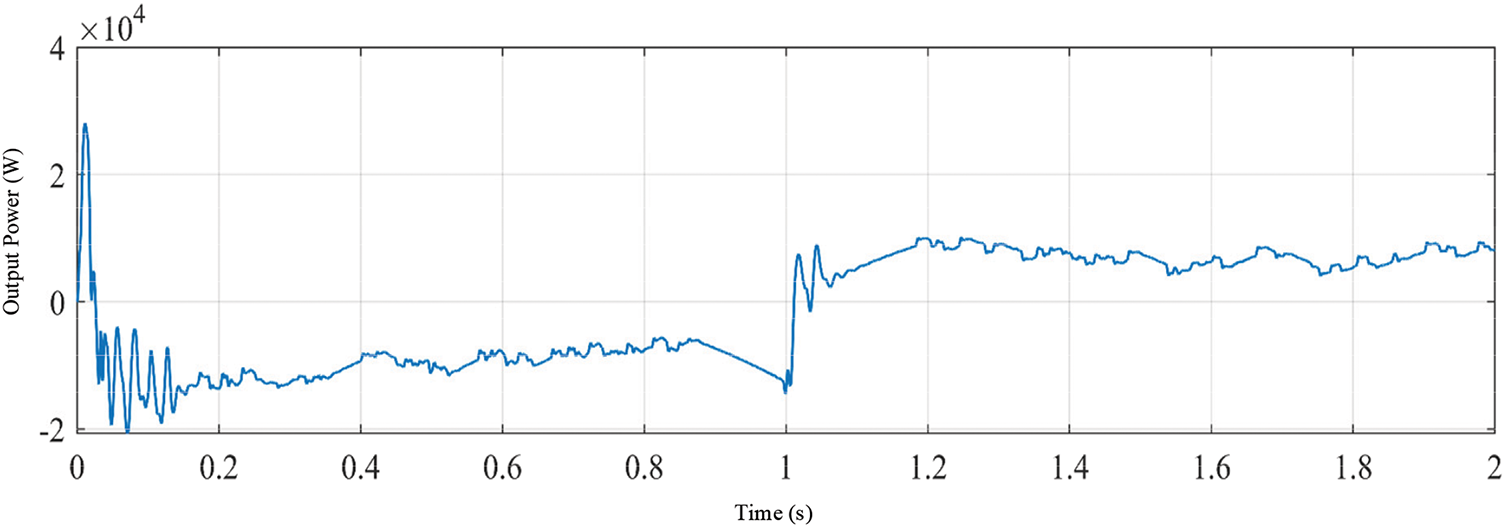
Figure 30: Battery output power

As can be seen from Fig. 31, the power consumption of the DC load fluctuates with changes in the environment, but has always been stable at around 15 kW, and the power on the DC bus is in a dynamic balance state.

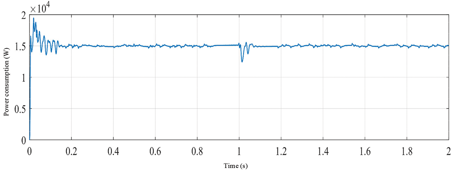
Figure 31: DC load power consumption

As shown in Fig. 32, during the startup phase, the state of charge of the battery has a slight downward trend, which corresponds to the discharge step in Fig. 32. Before 1 s, the state of charge is on an upward trend, indicating that the battery is in a charging state; after 1 s, the state of charge is on a downward trend, indicating that the battery is in a discharging state.

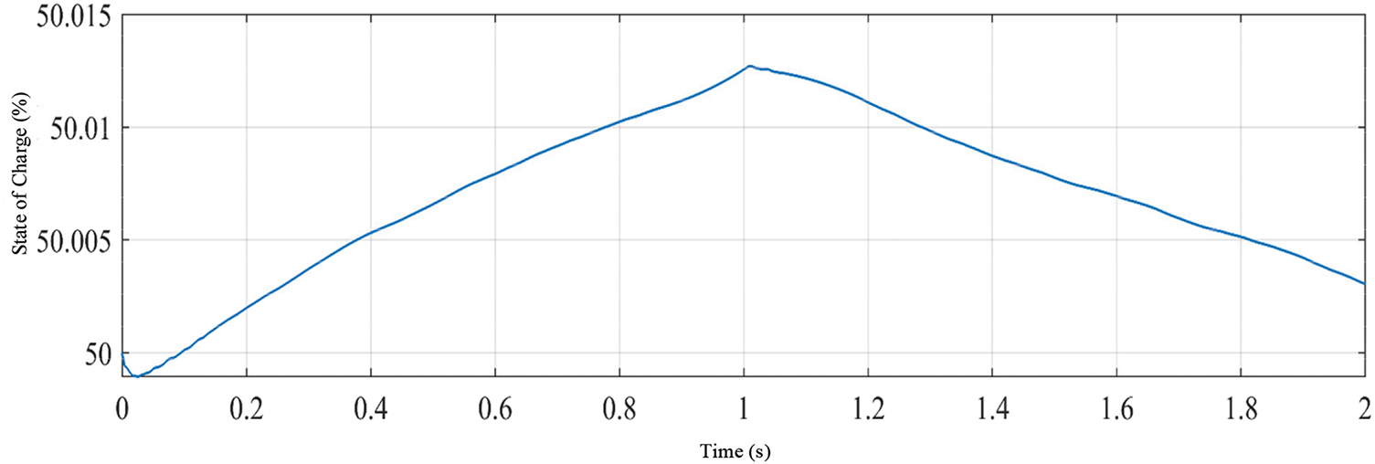
Figure 32: Battery state of charge

As shown in Fig. 33, the DC bus voltage has been maintained at around 380 V, which shows that the constant voltage control strategy based on the Buck/Boost converter can well control the DC bus within a constant value. In summary, the GFISMC algorithm and the UIGWO-INC algorithm can quickly stabilize the output power of the offshore wind-solar hybrid power generation system near the maximum power point when external conditions change.

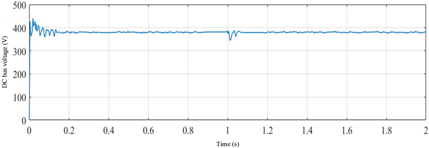
Figure 33: Voltage on the DC bus

4  Simulation Analysis Based on Semi-Physical Simulation Platform

4.1 Introduction to Semi-Physical Simulation Platform and Simulation Process

Due to the large number of subsystems and circuit components in the offshore wind-solar hybrid power generation system, if the algorithm proposed in this study is directly used to test the actual offshore wind-solar hybrid power generation system, it may damage the original equipment, resulting in high cost and low efficiency. Therefore, in order to quickly and cost-effectively verify the feasibility and effectiveness of the control strategy mentioned above, this study conducted semi-physical simulation verification on the ModelingTech power electronics experimental system developed by Yuankuan Energy Technology Co., Ltd. The hardware structure of the semi-physical simulation system is shown in Fig. 34.

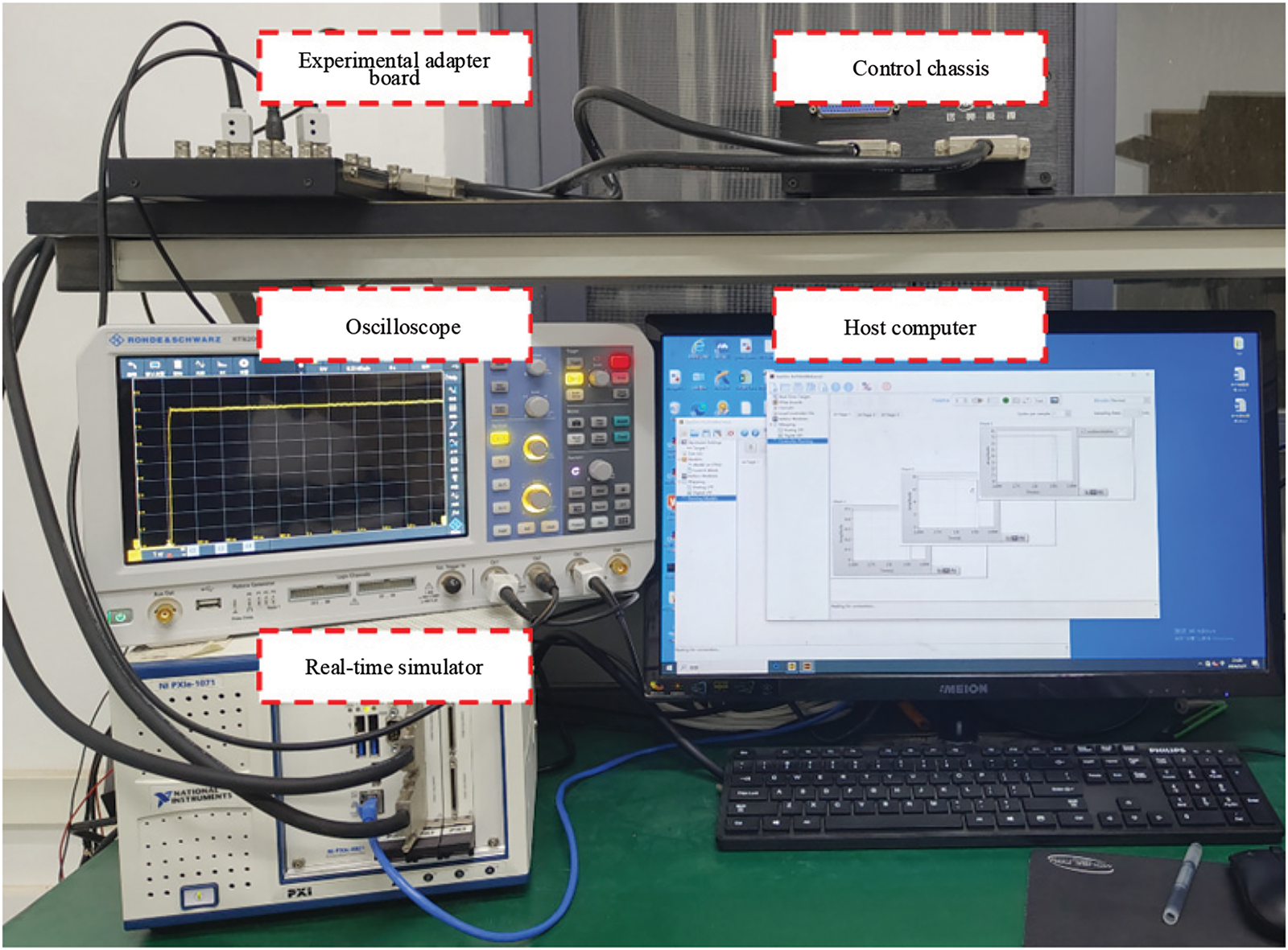
Figure 34: Overall architecture of the semi-physical simulation system

As shown in Fig. 34, the hardware of the semi-physical simulation system mainly consists of four parts: control chassis, real-time simulation chassis, experimental adapter board, and oscilloscope:

(1)   The control chassis is mainly used to generate and transmit control signals. This chassis has a built-in embedded controller. The controller is based on the ZYNQ architecture and uses the NI Linux Real-Time operating system, Artix-7 FPGA, and a dual-core ARM Cortex-A9 processor with a main frequency of 667 MHz to achieve real-time control and high-performance computing. In addition, the control chassis is also equipped with 32 LVTTL digital I/O interfaces, 8 1 kS/s low-speed analog output interfaces, and 16 100 kS/s high-speed synchronous analog sampling input interfaces.

(2)   The core function of the real-time simulation chassis is to perform high-precision real-time simulation. The real-time simulation chassis is designed based on a 4-slot 3U PXI Express chassis architecture with a bandwidth of up to 1 GB/s (dedicated) and 3 GB/s (system) per slot. It is equipped with Kintex-7 160 T series FPGA chip, Intel i3 series dual-core 2.6 GHz CPU, 2 GB memory, and integrated USB, serial port and Gigabit Ethernet interface. In addition, the chassis provides 8 16-bit ±10 V 500 kS/s analog input interfaces, 8 16-bit ± 10 V 1 MS/s analog output interfaces, 32 10 MHz 3.3 V TTL digital input interfaces and 8 10 MHz 3.3 V TTL digital output interfaces.

(3)   The main function of the experimental adapter board is to connect the control end and the simulation end and transmit signals between the two ends. One end is connected to the simulator through the SCSI-68 pin interface, and the other end is connected to the control chassis through the DB-37 interface to form a signal channel. The adapter board is equipped with 24 BNC interfaces, which are divided into three groups: 8 interfaces correspond to the low-speed analog output signals of the control end, 8 interfaces correspond to the digital I/O signals of the simulation end, and 8 interfaces correspond to the analog output signals of the simulation end.

(4)   The oscilloscope is mainly used to monitor the target signal waveform in real time. The oscilloscope has a 10-bit vertical resolution, a sensitivity of 1 mV/div, a sampling rate of 2.5 GS/s, and a maximum storage depth of 20 Msample.

The software part of the semi-physical simulation system mainly consists of StarSim HIL and StarSim RCP, as shown in Figs. 35 and 36. StarSim HIL is a configuration-type model management software that can load Simulink models onto the hardware of the real-time simulation chassis. StarSim RCP is a model management software for rapid control prototyping that can load the control algorithm model code written in Simulink onto the hardware of the control chassis.

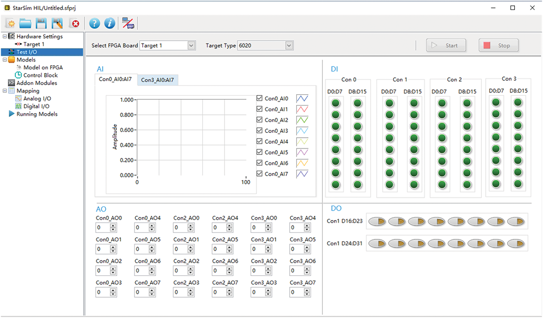
Figure 35: The interface of the StarSim HIL software

Figure 36: The interface of the StarSim RCP software

Based on the above hardware and software, the semi-physical simulation process of the offshore wind-solar hybrid power generation system can be roughly illustrated by the following Fig. 37.

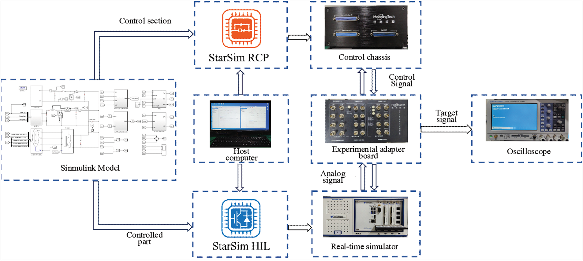
Figure 37: Schematic diagram of the semi-physical simulation process

First, the Simulink model of the offshore wind-solar hybrid power generation system is split into the controlled part and the control part, and the input and output are set. The controlled part is the main circuit model of the offshore wind-solar hybrid power generation system, as shown in Fig. 38; the control part is the control algorithm model of each part, which needs to be converted into a dll file through Simulink, as shown in Fig. 39.

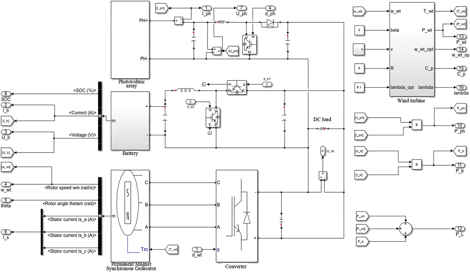
Figure 38: Controlled part of the offshore wind-solar hybrid power generation system

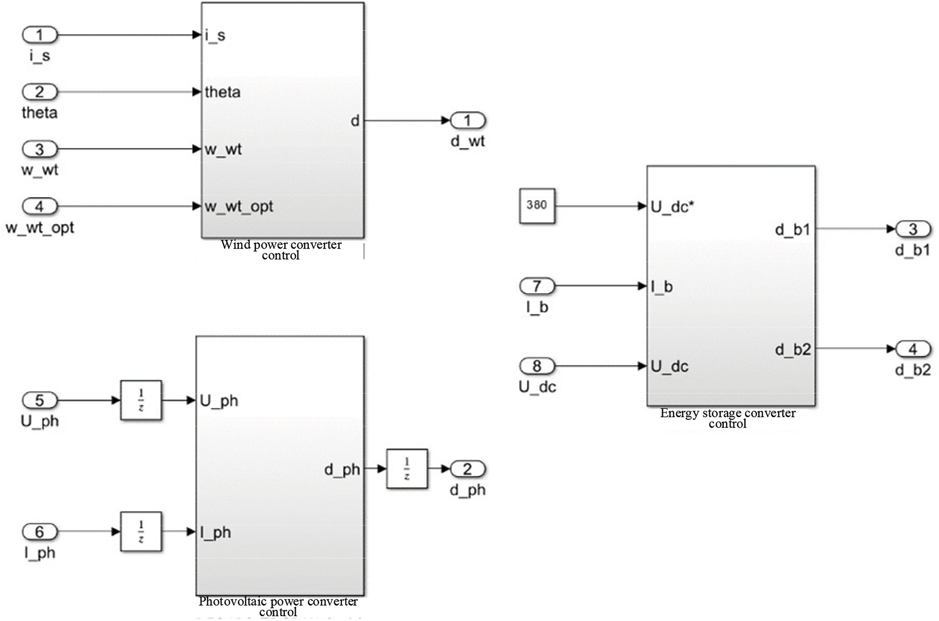
Figure 39: Control section of the offshore wind-solar hybrid power generation system

Then, start the real-time simulation chassis and the control chassis, and communicate with the host computer by entering the IP address. Load the Simulink model of the controlled part into StarSim HIL in the host computer, and load the dll file of the control part into StarSim RCP. Then, through the visual I/O configuration, match the input and output signals of the model with the input and output interfaces of the two chassis, as shown in Figs. 40 and 41.

Figure 40: Schematic diagram of interface matching of the controlled part

Figure 41: Schematic diagram of the control part interface matching

After the preparation is completed, the control part is first loaded onto the CPU of the control chassis using StarSim RCP software, and then the controlled part is loaded onto the FPGA of the real-time simulation chassis using StarSim HIL software. When the entire system is running, the target signal can be observed with the help of an oscilloscope, as shown in Fig. 41, and the signal data can also be collected using the host computer interface for real-time observation, as shown in Fig. 42.

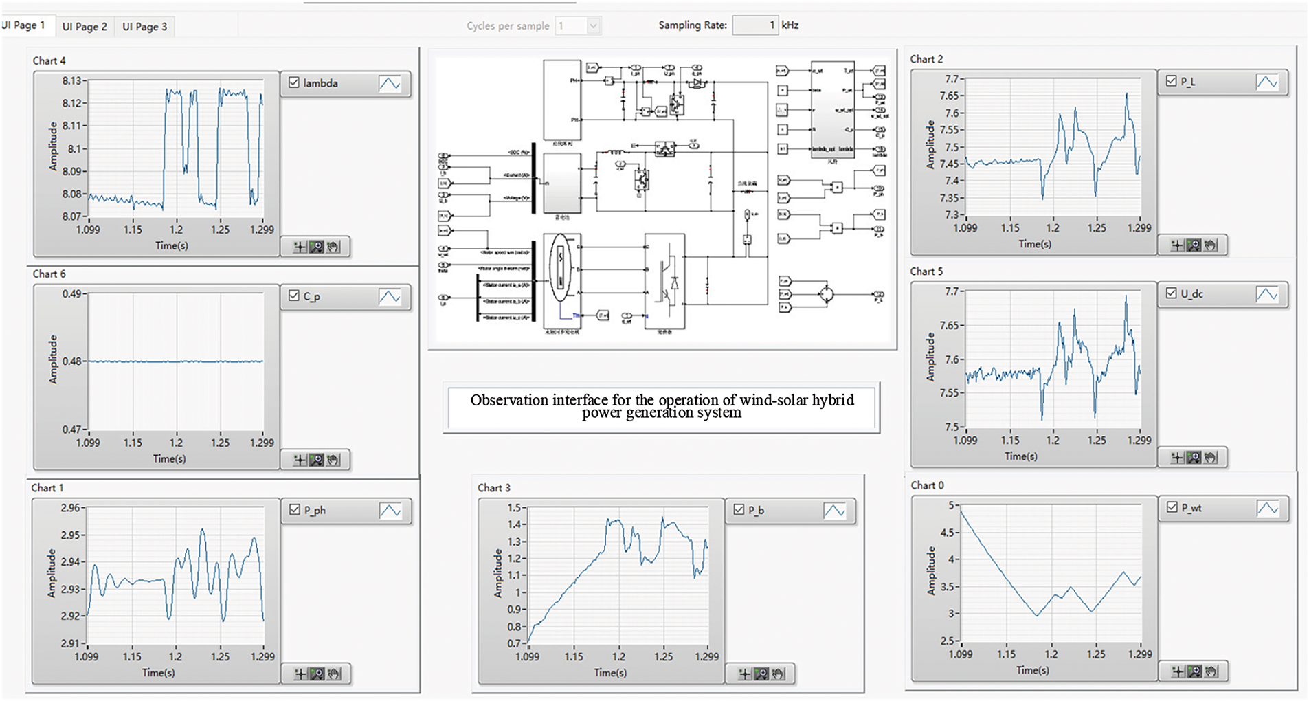
Figure 42: Observation interface of the operation of offshore wind-solar hybrid power generation system

4.2 Results of Semi-Physical Simulation

In order to verify the correctness and rationality of the simulation model built in the previous section, the key parameters and working conditions of the offshore wind-solar hybrid power generation system model in the semi-physical simulation process are the same as those in the previous section, and the target signal input to the oscilloscope is also the same key indicator signal. Since the voltage range of the analog output of the real-time simulation chassis is limited to between −10 and 10 V, the key indicator signal can only be fully output to the oscilloscope for display after being reduced. The horizontal axis scale value of the oscilloscope is set to 200 ms, and the overall simulation is 2.2 s. In addition, since the key indicator signal curve needs to be manually captured in the oscilloscope, there will be a slight offset in the time correspondence, but the overall change trend and the size of the vertical axis will not be affected. Based on the above foundation, the simulation results under the semi-physical simulation platform are shown in Figs. 43 to 46. Since the minimum scale of the oscilloscope vertical axis is 1 mV and the SOC change amplitude of the battery is small, the change of the SOC indicator will not be analyzed.

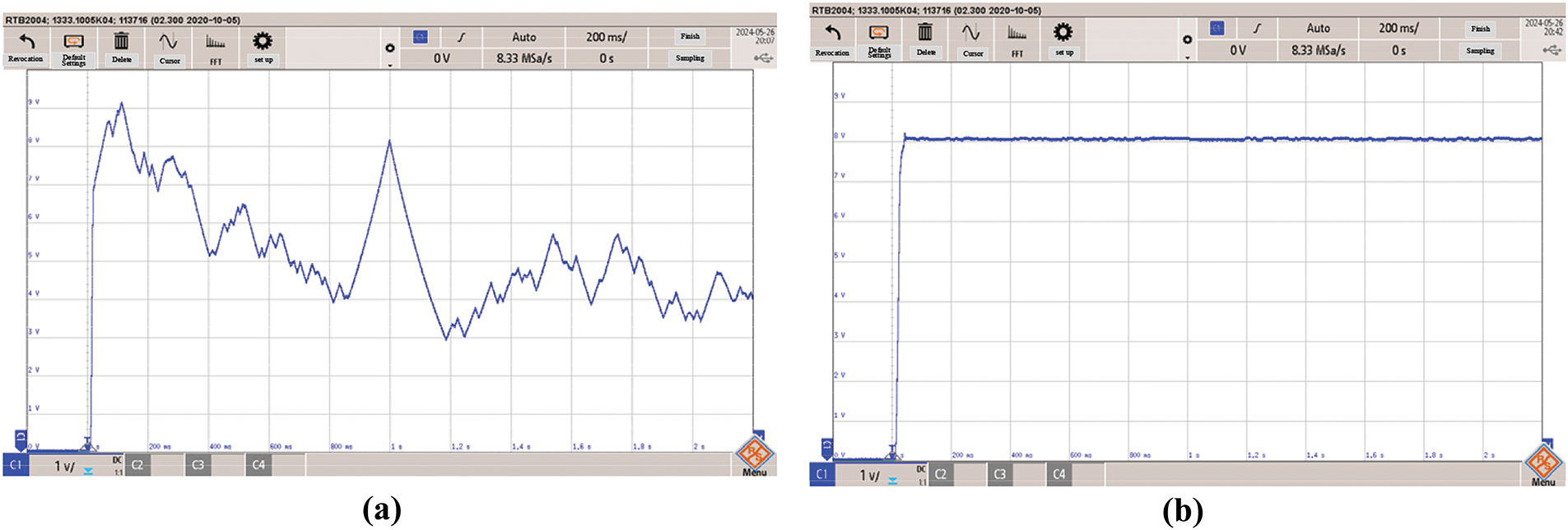
Figure 43: Offshore wind turbine output power and tip speed ratio under semi-physical simulation. (a) Offshore wind turbine output power. (b) Tip speed ratio

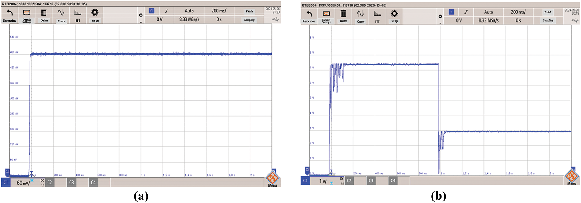
Figure 44: Wind energy utilization coefficient and offshore photovoltaic array output power under semi-physical simulation. (a) Wind energy utilization coefficient. (b) Offshore photovoltaic array output power

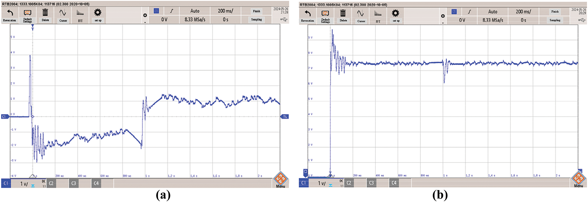
Figure 45: Battery output power and DC load power consumption under semi-physical simulation. (a) Battery output power. (b) DC load power consumption

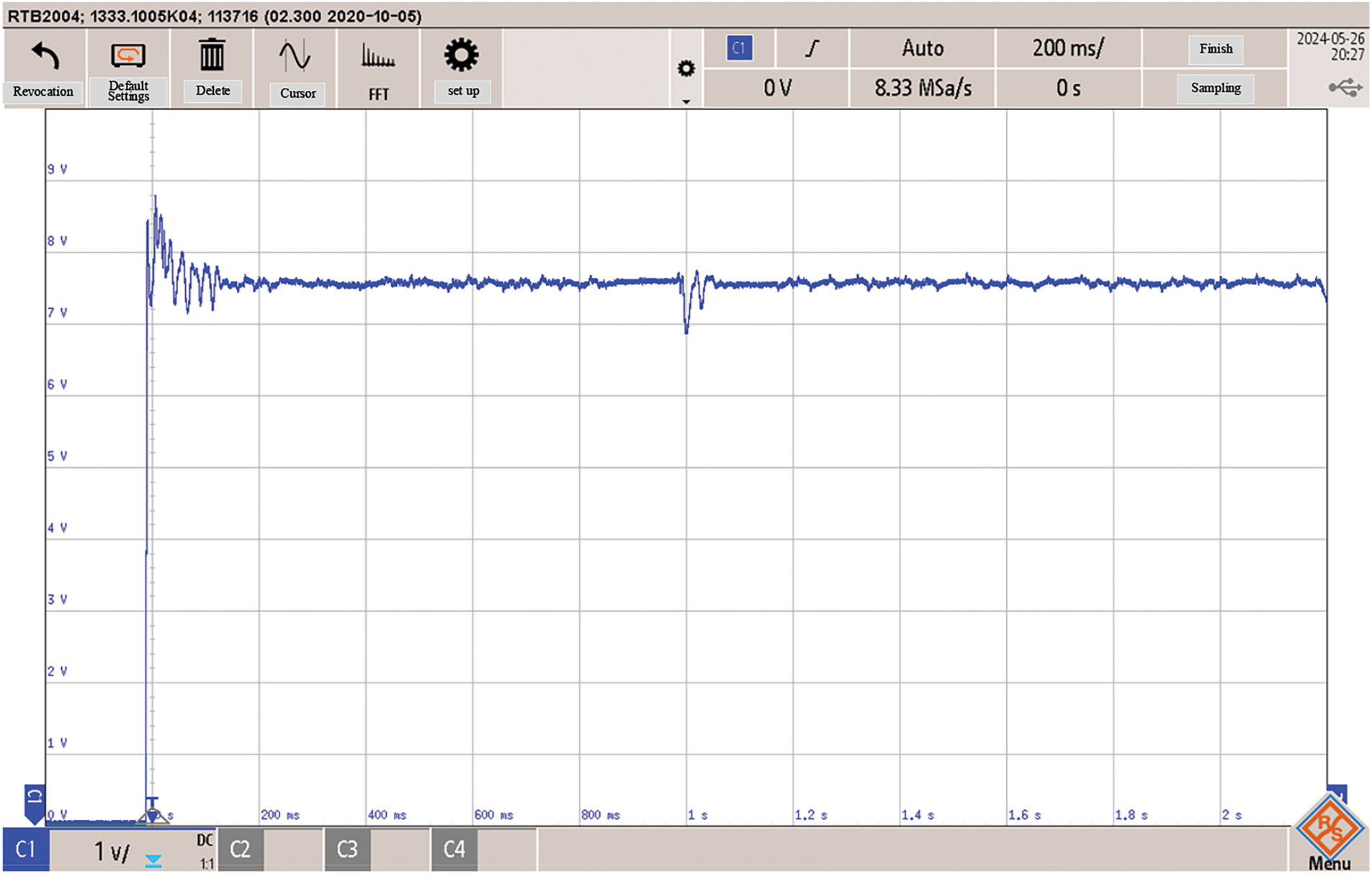
Figure 46: DC bus voltage under semi-physical simulation

The vertical axis scale values in Fig. 43 are all 1 V, and the first scale is also 0 V. In Fig. 43a, the displayed value of the offshore wind turbine output power is 1/1100 of its original analog signal, and its overall trend changes with the wind speed. In Fig. 43b, the displayed value of the tip speed ratio is the same as its original analog signal, and has been stable at the optimal tip speed ratio of about 8.1.

The first scale of the vertical axis in Fig. 44 is 0 V. The scale value of the vertical axis in Fig. 44a is 0.1 V, where the displayed value of the wind energy utilization coefficient is the same as its original analog signal, and has been stable at around the maximum wind energy utilization coefficient of 0.48. Its optimal tip speed ratio with the above figure fully demonstrates that the proposed algorithm can enable the offshore wind power generation module to track the maximum power point. The scale value of the vertical axis in Fig. 44b is 1 V, and the value of the output power of the offshore photovoltaic array is 1/2000 of its original analog signal. Through conversion, it is known that the output power of the offshore photovoltaic array in the first and second stages can quickly stabilize near their respective maximum power points, which are 14,357 and 5832 W, respectively.

The vertical axis scale values in Fig. 45 are all 1 V. The first scale of the vertical axis in Fig. 45a is −4 V, and the value of the battery output power is 1/7000 of its original analog signal. The battery output power is in the charging state in the first stage and in the discharging state in the second stage. The first scale of the vertical axis in Fig. 45b is 0 V, and the value of the DC load power consumption is 1/2000 of its original analog signal. It can be seen from the conversion that the DC load power consumption is dynamically stable at about 15 kW. The vertical axis scale value in Fig. 46 is 1 V, the first scale is 0 V, and the value of the DC bus voltage is 1/50 of its original analog signal. It can be seen from the conversion that the DC bus voltage has been dynamically stable at about 380 V. In summary, the results of the semi-physical simulation curve fully prove that under random wind speed and dynamic local shadow, the algorithm proposed in this study can quickly and effectively track the maximum power point of the offshore wind-solar hybrid power generation system. The trends and specific values of each key indicator also indirectly verify the rationality and correctness of the MATLAB/Simulink simulation model built in the previous section.

5  Conclusion

This study focuses on the maximum power point tracking control of offshore wind-solar hybrid power generation systems. First, the mathematical model, working characteristics, and corresponding control strategies of wind and solar power generation systems are analyzed. Then, based on this, the MPPT control algorithm is improved. Finally, MATLAB/Simulink is used to build the integrated simulation model of each independent part and system, and the improved algorithm is verified under different working conditions with the help of this platform and the semi-physical simulation platform. The main work completed in this study is summarized as follows:

(i)   The MPPT control method of offshore wind power generation system is improved. In view of the fact that the offshore wind power generation system has a maximum power point at each wind speed, this study studies the sliding mode control algorithm based on the tip speed ratio method and proposes a global fast integral sliding mode control algorithm (GFISMC). The algorithm adopts a fast integral sliding mode surface and a fuzzy fast switching control term so that the system state error variable converges quickly to 0. In the process of designing the switching control term, in order to solve the problem of chattering, this study uses the sign function to replace the original sign function and adds a fuzzy compensation coefficient, which not only reduces the chattering but also increases the anti-interference ability of the sliding mode control. Finally, a simulation model of an offshore wind power generation system was built in MATLAB/Simulink. The fast tracking and low jitter properties of the algorithm were verified through comparative experiments under step wind speed and random wind speed.

(ii)   The feasibility and effectiveness of the improved algorithm were verified in an offshore wind-solar hybrid power generation system. The working mode of the off-grid offshore wind-solar hybrid power generation system was analyzed, and the working mode in the MPPT control state was selected. Subsequently, a complete offshore wind-solar hybrid power generation system model was built using MATLAB/Simulink, and the semi-physical simulation platform was used to simulate the selected working mode and the feasibility and effectiveness of the improved MPPT control algorithm were fully verified.

This study mainly studies the MPPT control method of the offshore wind-solar hybrid power generation system and verifies the algorithm effect through a series of simulations. Improvements and improvements are needed, mainly including the following aspects:

(i)   This study focuses on the MPPT control method under the condition of continuous fluctuations in wind speed and light intensity but ignores the economic cost control of offshore wind and offshore photovoltaic power generation, as well as the overall coordinated optimization of the offshore wind-solar hybrid power generation system. In the future, research in these areas can be carried out based on this study so as to further improve the economic benefits and overall performance of the system.

(ii)   Although the research content of this study was verified on the MATLAB/Simulink simulation platform and the semi-physical simulation platform, the verified working conditions were relatively simple. In subsequent research, more complex load conditions and off-grid conditions can be considered, and a full-physical hardware platform can also be built for experimental verification.

(iii)   The actual deployment scenarios of this algorithm in real-world offshore wind-solar systems are still improving. Potential engineering limitations, such as computational complexity in complex environments, parameter sensitivity, or hardware feasibility, need to be gradually addressed.

Acknowledgement: This work was supported by the 2022 Sanya Science and Technology Innovation Project, China, the Sanya Science and Education Innovation Park, Wuhan University of Technology, China and the Hainan Provincial Joint Project of Sanya Yazhou Bay Science and Technology City, China.

Funding Statement: This work was supported by the 2022 Sanya Science and Technology Innovation Project, China (No. 2022KJCX03), the Sanya Science and Education Innovation Park, Wuhan University of Technology, China (Grant No. 2022KF0028) and the Hainan Provincial Joint Project of Sanya Yazhou Bay Science and Technology City, China (Grant No. 2021JJLH0036).

Author Contributions: Conceptualization, Xiangyang Cao, Yaojie Zheng; methodology, Hanbin Xiao, Min Xiao; software, Xiangyang Cao, Yaojie Zheng; validation, Hanbin Xiao, Min Xiao; formal analysis, Xiangyang Cao, Yaojie Zheng; investigation, Hanbin Xiao, Min Xiao; resources, Xiangyang Cao, Yaojie Zheng; data curation, Hanbin Xiao, Min Xiao; writing—original draft preparation, Xiangyang Cao, Yaojie Zheng; writing—review and editing, Hanbin Xiao, Min Xiao; visualization, Xiangyang Cao, Yaojie Zheng; supervision, Hanbin Xiao; project administration, Min Xiao; funding acquisition, Min Xiao. All authors reviewed the results and approved the final version of the manuscript.

Availability of Data and Materials: Data available on request from the authors.

Ethics Approval: Not applicable.

Conflicts of Interest: The authors declare no conflicts of interest to report regarding the present study.

References

1. Yin X, Lei M. Jointly improving energy efficiency and smoothing power oscillations of integrated offshore wind and photovoltaic power: a deep reinforcement learning approach. Prot Control Mod Power Syst. 2023;8(1):25. doi:10.1186/s41601-023-00298-7. [Google Scholar] [CrossRef]

2. Tang W, Xu S, Zhou X, Yang K, Wang Y, Qin J, et al. Meeting China’s electricity demand with renewable energy over Tibetan Plateau. Sci Bull. 2023;68(1):39–42. doi:10.1016/j.scib.2022.12.012. [Google Scholar] [PubMed] [CrossRef]

3. Guo X, Dong Y, Ren D. CO2 emission reduction effect of photovoltaic industry through 2060 in China. Energy. 2023;269:126692. doi:10.1016/j.energy.2023.126692. [Google Scholar] [CrossRef]

4. Wei D, Wei P, Li D, Ying Z, Hao X, Xue Z. Intelligent damping control of renewable energy/hydrogen energy DC interconnection system. Energy Rep. 2022;8(6):972–82. doi:10.1016/j.egyr.2022.10.306. [Google Scholar] [CrossRef]

5. Liu S, You H, Liu Y, Feng W, Fu S. Research on optimal control strategy of wind-solar hybrid system based on power prediction. ISA Trans. 2022;123(3):179–87. doi:10.1016/j.isatra.2021.05.010. [Google Scholar] [PubMed] [CrossRef]

6. Zhang J, Song J, Liu J, Lin J. Bridge type grab ship unloaders. In: Handbook of port machinery 2024. Singapore: Springer Nature Singapore; 2024. p. 363–450. [Google Scholar]

7. Huang G, Tang Y, Chen X, Chen M, Jiang Y. A comprehensive review of floating solar plants and potentials for offshore applications. J Mar Sci Eng. 2023;11(11):2064. doi:10.3390/jmse11112064. [Google Scholar] [CrossRef]

8. Marzebali MH, Mazidi M, Mohiti M. An adaptive droop-based control strategy for fuel cell-battery hybrid energy storage system to support primary frequency in stand-alone microgrids. J Energy Storage. 2020;27:101127. doi:10.1016/j.est.2019.101127. [Google Scholar] [CrossRef]

9. Liao X, Wang Y, Du Y, Xiao S, Liu X, Zhu Z, et al. An 85.5% PCE and 99.31% TE piezoelectric energy harvesting interface with sub-one-cycle sampling and dual-loop MPPT. IEEE Trans Circuits Syst II Express Briefs. 2025;72(3):444–8. doi:10.1109/TCSII.2025.3530088. [Google Scholar] [CrossRef]

10. Liang Z, Liang Y, Luo X, Yu Z, Chen J, Chen Y. Multi-objective optimization of proton exchange membrane fuel cell based methanol-solar-to-X hybrid energy systems. Appl Energy. 2024;373(1):123828. doi:10.1016/j.apenergy.2024.123828. [Google Scholar] [CrossRef]

11. Youssef AR, Mousa HHH, Saeed MSR, Ali A, Shaaban MF, Mohamed EEM, et al. A novel self-adjustable robust MPPT strategy for two-stage grid-integrated solar PV systems. Electr Eng. 2024;308(1):634. doi:10.1007/s00202-024-02858-y. [Google Scholar] [CrossRef]

12. Prabhakar K, Jain SK, Padhy PK. Inertia estimation in modern power system: a comprehensive review. Electr Power Syst Res. 2022;211(1):108222. doi:10.1016/j.epsr.2022.108222. [Google Scholar] [CrossRef]

13. Hong F, Wei K, Ji W, Hao J, Fang F, Liu J. A cross-entropy-based synergy method for capacity configuration and SOC management of flywheel energy storage in primary frequency regulation. Energy. 2025;316(9):134498. doi:10.1016/j.energy.2025.134498. [Google Scholar] [CrossRef]

14. Witthohn R. Offshore work. In: International shipping: the role of sea transport in the global economy. Wiesbaden, Germany: Springer Fachmedien Wiesbaden; 2022. p. 491–541. [Google Scholar]

15. Mohamedy Ali MH, Sayed Mohamed MM, Ahmed NM, Zahran MBA. Comparison between P&O and SSO techniques based MPPT algorithm for photovoltaic systems. Int J Electr Comput Eng IJECE. 2022;12(1):32. doi:10.11591/ijece.v12i1.pp32-40. [Google Scholar] [CrossRef]

16. Li K, Wu Y, Wei L. Simulation of photovoltaic system’s artificial intelligence control or based on fuzzy perturbation algorithms. Int J Comput Appl Technol. 2022;70(1):22. doi:10.1504/IJCAT.2022.129892. [Google Scholar] [CrossRef]

17. Shangguan XC, Shi S, He Y, Zhang CK. Optimal digital load frequency control of smart grid considering sampling and time delay based on warm-up gray wolf algorithm. IEEE Trans Ind Inform. 2025;21(2):1773–82. doi:10.1109/TII.2024.3485821. [Google Scholar] [CrossRef]

18. Jin Y, Guo H, Wang J, Song A. A hybrid system based on LSTM for short-term power load forecasting. Energies. 2020;13(23):6241. doi:10.3390/en13236241. [Google Scholar] [CrossRef]

19. Elbaksawi O, Elminshawy NAS, Diab S, Eltamaly AM, Mahmoud A, Elhadidy H. Innovative metaheuristic algorithm with comparative analysis of MPPT for 5.5 kW floating photovoltaic system. Process Saf Environ Prot. 2024;185:1072–88. doi:10.1016/j.psep.2024.03.082. [Google Scholar] [CrossRef]

20. Ding J, Lu C, Li B. A data-driven based security situational awareness framework for power systems. J Signal Process Syst. 2022;94(11):1159–68. doi:10.1007/s11265-022-01741-y. [Google Scholar] [CrossRef]

21. Ahmed MMR, Mirsaeidi S, Ali Koondhar M, Karami N, Tag-Eldin EM, Ghamry NA, et al. Mitigating uncertainty problems of renewable energy resources through efficient integration of hybrid solar PV/wind systems into power networks. IEEE Access. 2024;12(2):30311–28. doi:10.1109/ACCESS.2024.3370163. [Google Scholar] [CrossRef]

22. AL-Wesabi I, Fang Z, Cai J, Hussein Farh HM, Aboudrar I, Dagal I, et al. Fast DC-link voltage control based on power flow management using linear ADRC combined with hybrid salp particle swarm algorithm for PV/wind energy conversion system. Int J Hydrogen Energy. 2024;61:688–709. doi:10.1016/j.ijhydene.2024.02.325. [Google Scholar] [CrossRef]

23. Bassey KE. Hybrid renewable energy systems modeling. Eng Sci Technol J. 2023;4(6):571–88. doi:10.51594/estj.v4i6.1255. [Google Scholar] [CrossRef]

24. Chrifi-Alaoui L, Drid S, Ouriagli M, Mehdi D. Overview of photovoltaic and wind electrical power hybrid systems. Energies. 2023;16(12):4778. doi:10.3390/en16124778. [Google Scholar] [CrossRef]