MOCBOA: Multi-Objective Chef-Based Optimization Algorithm Using Hybrid Dominance Relations for Solving Engineering Design Problems

1  Introduction

An essential concept in several disciplines, such as engineering, economics, and artificial intelligence, is multi-objective optimization. These domains frequently feature situations where it’s necessary to simultaneously optimize several competing goals. For instance, it is typical in engineering design to have to balance performance with cost and weight reduction. It is difficult to develop solutions to such challenges that meet all of the objectives because of the inherent trade-offs. Even though several works have been presented to solve them [1,2], sophisticated multi-objective optimization approaches are required [3,4] due to their complexity in traversing these trade-offs and finding a set of balanced solutions.

Dominance relations, which offer a framework for assessing and contrasting alternatives, are essential to this process (Multi-objective optimization). These relations establish a solution’s relative superiority or inferiority based on how well it performs in comparison to other solutions across the given objectives. Therefore, the choice of a dominance relation strongly impacts the diversity, convergence, and efficiency of the optimization process. The most prevalent dominance relations include Pareto dominance, Epsilon dominance, Cone-epsilon dominance, and Strengthened dominance relations, each providing distinct benefits for various optimization problems. Given the widespread use of those relations as a foundational concept, several algorithms have been created to take advantage of them. Due to the extensive number of algorithms only the state-of-the-art ones are briefly reviewed here.

Probably the most well-known and frequently applied dominance notion is Pareto dominance. If a solution is better in at least one objective and not worse in any, it is said to Pareto-dominate another. Numerous multi-objective algorithms, such as the Non-dominated Sorting Genetic Algorithm II (NSGA-II) [5], are based on this idea. NSGA-II is well known for its ability to quickly sort non-dominated solutions using a crowding distance mechanism and a variety of Pareto-optimal solutions. In Strength Pareto Evolutionary Algorithm II (SPEA-II) [6], each solution is given a strength value by SPEA2, which indicates how many solutions it dominates. To preserve diversity, it also takes into consideration the density of solutions in the objective space. Multi-Objective Evolutionary Algorithm based on Decomposition (MOEA/D) [7] is also a known algorithm. In this algorithm, a multi-objective optimization issue is broken down by MOEA/D into many scalar optimization subproblems, which are then all optimized at the same time. The optimum answers to these subproblems are found using Pareto dominance. Multi-Objective Particle Swarm Optimization (MOPSO) [8] expands upon the standard single-objective PSO algorithm to enable it to handle multiple objectives. It updates the particle positions using Pareto dominance and a global repository of non-dominated solutions. Other techniques include Multi-Objective Grey Wolf Optimization (MOGWO) [9], Multi-Objective Cat Swarm Optimization (MOCSO) [10], and Multi-objective Cohort Intelligence (MOCI) [11].

Another dominance relation is Epsilon Dominance, a variation of Pareto Dominance. It introduces a tolerance level, ε (epsilon), to account for small variations within solutions in each objective. Some of the recent algorithms that use Epsilon dominance include Guided Multi-objective equilibrium optimizer (GMOEO) [12] which enhances exploration and diversity by updating solutions through Epsilon dominance, resulting in efficient movement towards the Pareto front. Another method named Guided Multi-objective Marine Predator Algorithm (GMOMPA) [13], is a modified MPA-based framework for addressing multi-objective optimization issues. It includes an external archive Epsilon dominance, a fast non-dominated solution, and crowding distance. to obtain non-dominated solutions, ensuring fast convergence towards the Pareto optimal. Multi-Objective Gaining–Sharing Knowledge optimization (MOGSK) [14] introduces the extended version of the gaining-sharing knowledge optimization (GSK), to tackle real-world optimization challenges. The algorithm utilizes an external archive population, fast nondominated sorting, and the Epsilon dominance relation to accomplish diversity, coverage, and convergence. The study in [15] investigates a co-evolutionary approach to determine the precise value of ε in multi-objective evolutionary algorithms (MOEAs). The authors in [16] present a new decomposition-based multi-objective evolutionary algorithm for complex Pareto fronts that uses a hybrid weighting technique and adaptive Epsilon dominance to achieve optimal diversity. By employing a population archive, crowding distance, and Epsilon dominance to direct search regions, the work in [17] expands the single objective Manta-Ray foraging optimization to multi-objective cases named (MOMRFO).

Cone-epsilon dominance relation is a variant of Epsilon dominance designed for optimization problems with three or more objectives, or many-objective optimization. It combines Epsilon dominance with a conical region of dominance. Different works discuss that Cone-epsilon dominance is a good method for evolutionary algorithms such as [18] and [19], where it increases the diversity of solutions and enhances the performance in evolutionary multi-objective optimization. Another work that has employed this method is [12], which presents a comparison with Epsilon dominance relation.

Strengthened dominance relation also known as (SDR) is an advanced approach generally used in MOEAs, especially when tackling optimization problems with many different objectives (more than three). It is intended to enhance the selection process by striking a balance between two crucial factors: variety and convergence. Many works have employed SDR or its other variant in multi/many objectives optimization such as Multi-Objective Harris Hawks Optimization (MOHHO) [20], which solves multi-objective optimization problems using a Strengthened dominance relation. In [21], the performance of SDR is examined, and a new dominance relation (CSDR) based on SDR is proposed. In NSGA-II, the CSDR takes the place of Pareto dominance. In [22], a new Reference Points-based Strengthened dominance relation (RPS-dominance) has been introduced into NSGA-II. To differentiate and further stratify Pareto-equipment solutions, it presents a reference point set and the convergence metric. The Guided Differential Evolution method (MGDE) [23] is another approach to solving many objective optimization problems. It applies a Strengthened dominance relation and bi-goal evolution, as well as modified differential evolutionary operators for crossover and mutation. This guided exploration technique promotes convergence towards the Pareto front while maintaining good solution diversity.

A comprehensive review of existing multi-objective optimization algorithms is presented in Table 1. The table summarizes the dominance relations, key contributions, and relevance of each algorithm to the current study. While Pareto dominance is still the most commonly employed due to its simplicity and efficacy, Epsilon dominance and its variants provide more control over solution variety and convergence, especially in many-objective optimization. In contrast, stronger dominance relations address the issues of balancing convergence and diversity in complicated optimization environments. Although current algorithms such as NSGA-II, SPEA2, and MOEA/D have proved the efficacy of these dominance relationships, algorithm-specific evaluations are still required to find the most appropriate dominance strategy for emerging optimization strategies. These evaluations are critical for customizing dominance relations to the specific needs of new algorithms and problem contexts.

Building on these insights, in this work we present an extension of the Chef-Based Optimization Algorithm (CBOA) [25] called the Multi-objective Chef-Based Optimization Algorithm (MOCBOA) to tackle multi-objective optimization problems. MOCBOA incorporates mechanisms such as an external archive, fast non-dominated sorting (FNS), and crowding distance (CD) to ensure a robust performance. A key contribution of this work is the systematic comparison of four dominance relations, Pareto dominance, Epsilon dominance, Cone-epsilon dominance, and Strengthened dominance to determine the most effective strategy for updating archive solutions in MOCBOA. This comprehensive evaluation addresses a gap in the literature, by conducting a systematic comparison of all four dominance relations.

This work’s specific contributions include the following:

•   Extension of CBOA to Multi-Objective Optimization: We propose MOCBOA, the first multi-objective extension of the Chef-Based Optimization Algorithm. MOCBOA uses an external archive to store the non-dominated solutions and lead the total solutions to the best Pareto front.

•   Diversity and Convergence: To maintain diversity, assure solutions convergence, and guarantee an effective solution distribution, MOCBOA uses the FNS and crowding distance.

•   Systematic Comparison of Dominance Relations: The performance of the four dominance relations Pareto dominance, Epsilon dominance, Cone-epsilon dominance, and Strengthened dominance in the context of MOCBOA is compared through an experimental study while used to update the archive solutions. In order to assist in selecting the best approach for a particular optimization problem, this study offers insights into each dominance relation.

•   Validation on Real-World Problems Benchmark: We validate the effectiveness of MOCBOA on a wide range of Real-World constrained MOPs (RWMOPs) including mechanical design, chemical engineering, process, design, and synthesis, power electronics, and power systems.

•   Impact: By providing a robust and versatile tool for solving complex MOPs, MOCBOA addresses real-world challenges in engineering and other domains. The algorithm’s ability to adapt to different dominance relations and problem contexts makes it a valuable contribution to the field of multi-objective optimization. Our results underscore that the choice of a dominance relation significantly shapes the optimization outcomes, influencing both solution diversity and convergence toward the Pareto front.

As shown in Fig. 1, the rest of the paper is structured as follows: Section 2 covers the mathematical background of MOPs, Pareto dominance, Epsilon dominance, Cone-epsilon dominance, and Strengthened dominance. Section 3 presents the single-objective version of the CBOA algorithm. Section 4 introduces the proposed MOCBOA algorithm. Section 5 presents the findings and discussion. Finally, some conclusions are conveyed in Section 6.

Figure 1: Paper structure

2  Mathematical Background

This section contains definitions for concepts such as information on MOPs and Pareto dominance, Epsilon dominance, Cone-epsilon dominance, and Strengthened dominance relations.

2.1 Multi-Objective Optimization Problems

Simultaneously gathering and optimizing opposing objective functions is a systematic procedure known as multi-objective optimization. Depending on the problem’s nature, optimization may include maximization or minimization of an objective. Such a minimization problem can be formulated as follows:

(1)

subject to:

(2)

(3)

(4)

where the solution for the decision variables is denoted by , while meeting the equality constraints for and the inequality constraints for . The value denotes the number of objective functions. Furthermore, and stand for lower and upper bounds, respectively.

2.2 Pareto Dominance

Using the relational arithmetic operators to compare the produced solutions in a MOP proved to be challenging. Consequently, the idea of Pareto optimal dominance offered a straightforward method for contrasting options in the multi-objective search space. Moreover, the search space had a collection of Pareto optimal solutions instead of a single optimum solution with a Pareto front image. The key concepts of the Pareto dominance relation are as follows:

Definition 1. Pareto dominance: Consider two solutions and . is considered to dominate (noted as: ) if:

(5)

Definition 2. Non-dominated set: Non-dominated solutions are those that are not dominated by any other solution. Let be a set of solutions including non-dominated solutions as members. , denotes the set of solutions that are not dominated by any other solution from the set .

Definition 3. Pareto optimal set: The Pareto optimal set represents a collection of all non-dominated solutions in the search space.

2.3 Epsilon Dominance

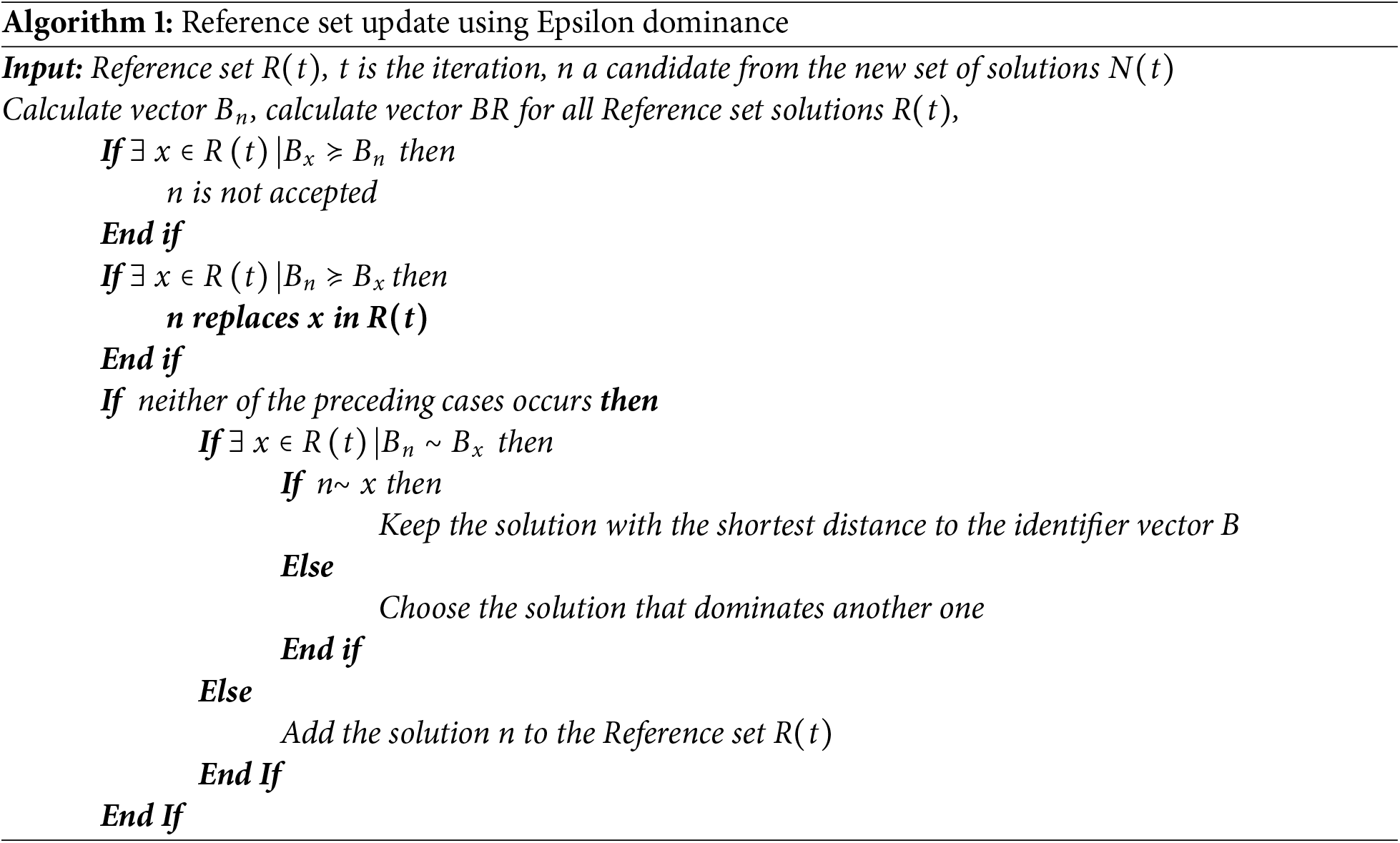
Laumanns et al. [24] presented the Epsilon dominance (-dominance) technique, which uses a two-level selection process to keep a representative and diverse group of solutions for multi-objective optimization. Using this method, the objective space is divided into hyper-boxes, each of which has a single solution vector. The box-level dominance relation guarantees the preservation of a set of non-dominated boxes. The objective space is first divided into hyper-boxes, and a vector B identifies each box. Every solution in the reference set is represented by this vector. Simultaneously, another set of solutions, , is taken into consideration, wherein denotes the identification vector linked to the objectives and is expressed as follows:

(6)

where stands for the permitted error, indicates the objective cost of the solution, and indicates the absolute value.

Let be updated according to Epsilon dominance using a new set of solutions denoted as , following the computation of the identification vectors for the new set of solutions, the -dominance relation is used to compare each new solution with the solutions from the reference set that already exist. Whether a new solution belongs to the reference set or not is decided by this comparison. To be more precise, the new solution n is admitted into the reference set, and the associated reference solution Ri is eliminated if the new solution’s identification vector dominates any identification vector of a solution in the reference set. In contrast, the new solution gets rejected if any of the dominates . A supplementary process is used if neither of these scenarios is valid (that is, if and are incomparable): if the new solution n dominates the reference solution in regular dominance, then n is accepted. If no answer dominates another one, the option that is closest to B is selected. Algorithm 1 presents the update process using the Epsilon dominance relation.

2.4 Cone-Epsilon Dominance

Cone-epsilon dominance, a more flexible form of Pareto dominance that falls under the larger category of relaxed dominance, was first proposed by Batista et al. [19]. Ikeda et al. [26] first proposed relaxed dominance to deal with situations in which a solution has a relatively low value in one objective, making it challenging to dominate. This was further refined by Ikeda et al. by adaptation of the α-dominance technique, which defines upper and lower bounds between two primary objectives using linear trade-off functions. This method enables a more flexible selection of non-dominated solutions, allowing a solution that would normally be rejected by standard Pareto dominance to dominate another one if it is significantly better in one objective but slightly inferior in another one.

Cone-epsilon dominance, which is based on relaxed dominance, is a hybrid form of both α- and -dominance. It makes use of cones to manage the dominance zone while attempting to maintain the convergence property of -dominance.

Definition 4. Cone: A set S is said to be a cone if λx∈S for any x ∈ S ∀ λ ≥ 0.

Definition 5. Generated cone for the vectors: and : the generated cone is the set:

(7)

With respect to dimension , and considering , it can be rewritten as follows:

(8)

Furthermore, in relation to the origins of the box and , the cone can be written as follows:

(9)

where represents the cone dominance matrix, and is a parameter that controls the cone opening.

Let the set be updated according to Cone-epsilon dominance using a new set of solutions denoted as , Cone-epsilon dominance creates hyper-boxes in the objective space, much like -dominance does. Additionally, it adjusts to two types of dominance: regular Pareto dominance and box-level dominance. With upper and lower bounds similar to the property adapted in α-dominance, the box contains a single unique identification vector, b. Each solution derived from R(t) and N(t) is now allocated a box, and b is determined as follows:

(10)

where ⌈.⌉ returns the closest upper integer to their argument and ⎣.⎦ returns the closest lower integer.

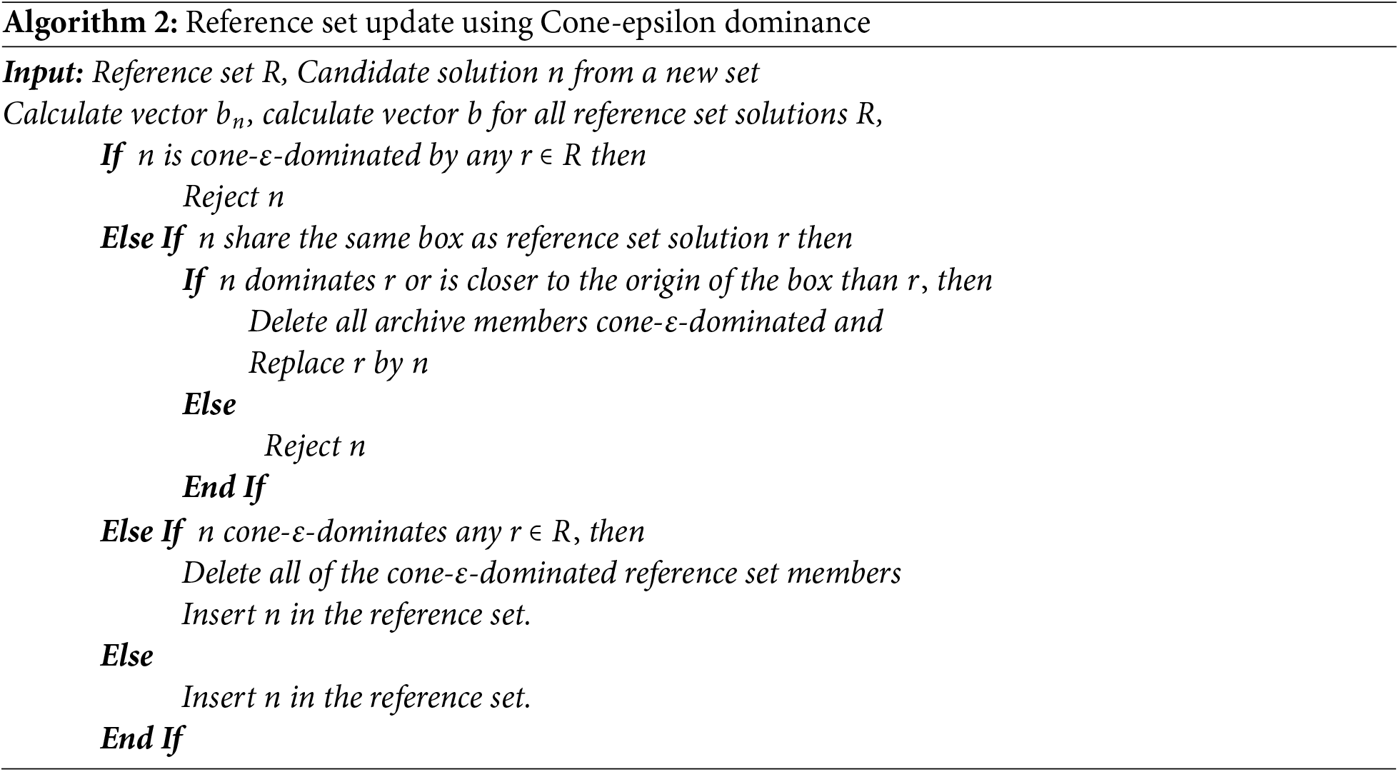
Dominance at the box level is now necessary to add a solution to the reference set. Consider two identification vectors of the solutions and the solutions, respectively, be and . The is said to cone--dominate only and only if Pareto dominates or the solution to the linear system is , with , , gives Similarly, we say if and only if:

(11)

A regular Pareto dominance is used when the identification vectors have the same box; the reference set solution is substituted only if the new set solution also exhibits Pareto dominance. If not, the closest point to the box’s origin is selected. The process for updating the reference set utilizing Cone-epsilon dominance is displayed in Algorithm 2.

2.5 Strengthened Dominance Relation (SDR)

As proposed by Tian et al. [27], the Strengthened dominance relation employs a customized niching strategy to achieve an optimal balance between the non-dominated solution set’s diversity and convergence. A potential solution is considered to be more dominant than another potential solution by SDR (represented as ) if and only if:

(12)

where determines the degree of convergence of , and it is expressed as Eq. (13). Furthermore, the acute angle between the two candidate solutions’ objective values is denoted by according to Eq. (14).

(13)

(14)

where indicates the niche size that each potential solution falls within. As per the first formula of Eq. (12), is considered to dominate when has a lower degree of convergence than and the angle between and any candidate solution is less than . According to the second formula of Eq. (12), the likelihood that will dominate is negatively correlated with the angle , however, if two candidate solutions, and , do not belong to the same niche, can dominate if has a lower degree of convergence than . As a result, the SDR relation does not penalize solution for choosing the solution with good convergence if the two candidate solutions, and , are in the same niche. If they are not, the SDR relation penalizes solution by a factor of to preserve diversity within the set of selected solutions. This dominance relation thereby facilitates improvements in both the convergence and diversity of the solutions.

3  Chef-Based Optimization Algorithm (CBOA)

Before introducing the extended proposed version (MOCBOA), we first introduce the original single-objective version. The CBOA [25] is a recently presented metaheuristic algorithm, inspired by the culinary school learning process. CBOA’s innovative approach is inspired by culinary training. Training programs offered by culinary schools are intended to improve students’ abilities and help them become skilled cooks. This iterative refinement of viable solutions to arrive at an ideal result is akin to the process of continuous improvement in metaheuristic algorithms. The conversion of student cooks into professional chefs is embodied by the CBOA framework, which includes various crucial components:

•   Chef Teachers: Each chef teacher at a cooking school is in charge of leading a class.

•   Class Selection: Students get to pick whatever classes they want to take, and their chef instructors will teach them a variety of cooking techniques.

•   Skill Refinement: With one-on-one instruction and supervision from a master chef instructor, chef instructors continuously enhance their abilities.

•   Students Learning: Students who study cooking strive to imitate and refine the methods that their chef instructors teach them, honing their skills via experience.

•   Graduation: After completing the program, culinary students are skilled cooks who have honed their craft through instruction.

Mathematical Model

The CBOA is a population-based algorithm that is divided into two groups: chefs and cooking students. Every component of the CBOA encapsulates details about the problem variables and suggests a potential solution. Each member of the CBOA is represented mathematically as a vector and can be modeled in a matrix. First, the population is initialized randomly, followed by the computation of the objective function for each member of the population. Then, the selection process of the different groups of chefs/students is done according to the objective function values, where the best results obtained will be selected as chefs while the remaining are selected as students. The population members of COBA must be updated with each iteration because the process is iterative. The update procedure varies depending on the group (chef/student) according to the following two phases:

•   Phase One: The competitive aspect of culinary expertise is shown by chefs striving to create quality ratings.

•   Phase Two: Students compete based on how well they can cook to get their quality ratings.

In phase one, the chefs adapt two strategies for an update: strategy one entails modeling themselves after the best chef teacher to learn their techniques, improves the algorithm by not depending only on the highest-ranking member of the population to train students, but also allowing the best chefs to hone their skills before instructing pupils. Additionally, through the prevention of the algorithm becoming stuck in local optima, this method allows the search space to be scanned more precisely and effectively. Eq. (15) determines each culinary teacher’s new position for with be the number of chefs and

(15)

where is the coordinate of the newly calculated position based on the first strategy (C/S1) of updating the chef instructor for the sorted member of the algorithm, is the coordinate of the best chef instructor, is a random number from the interval [0, 1], and is a number that is selected randomly during the execution from the set {1, 2}. This new position is acceptable if it improves the value of the objective function according to:

(16)

where is the objective function value associated with .

In the second phase, through individualized exercises and activities, the chef instructor aims to enhance his cooking abilities. attempts to find better solutions close to its location, regardless of the positions of other members of the population. It is possible that local search and exploitation, with slight adjustments to population members’ positions in the search space, can yield superior results. This idea states generating a random position around each instructor in the search space. This random position is appropriate for updating if it improves the objective function value.

(17)

(18)

where is an upper bound, is a lower bound, is the iteration count, is the new position, is the chef updating according to the second strategies and is the corresponding objective function value.

In the second phase, students adapt three tactics for updating: The first one is that each cooking student selects a class taught by a chef at random, and this chef instructor then teaches him cooking techniques. This results in students learning from the best and moving in the search space according to Eq. (20) and moving the students’ positions if the new objective function value is better:

(19)

(20)

where is the selected chef, is the students’ first updating strategy, and is randomly selected from the set .

The second tactic adapts a “skill” based update, where a random chef is selected and one of his variables is taken to replace one of the student’s variables. This variable is regarded as a skill.

(21)

(22)

The third updating tactic focuses on local search, where students try to improve all of their variables. Using a randomly generated position close to the student, similar to chef’s second strategy (Eqs. (17) and (18)) a new position is generated as follows:

(23)

where is the objective function value for the new position , and is the students’ third updating strategy.

The above-mentioned whole process is repeated until the stopping criterion is met.

4  Multi-Objective Chef-Based Optimization Algorithm (MOCBOA)

This section provides a detailed outline of the proposed MOCBOA algorithm. The core of MOCBOA is a mechanism for identifying non-dominated solutions by storing them in an external archive. The Pareto dominance relation plays a fundamental role in distinguishing non-dominated solutions, while the crowding distance metric enhances diversity among the solutions, promoting a well-distributed set along the Pareto front. Additionally, the FNS is incorporated to facilitate the generation of multiple Pareto fronts. To ensure that the archive remains up-to-date with the most relevant solutions, MOCBOA uses a combination of dominance relations to compare and refine the entries. In addition to the Pareto dominance, we employ Epsilon dominance to allow a degree of tolerance in solution comparisons, Cone-epsilon dominance to focus on solutions within a specific performance range, and Strengthened dominance to prioritize certain solution characteristics. Together, these strategies enable a robust approach to maintaining an archive that reflects a balanced and high-quality solution set throughout the optimization process. In summary, the employed approach covers multiple key points:

•   an external repository that can direct the candidates towards an optimal set and hold the best non-dominated solutions.

•   The update process of the archive’s solutions uses dominance relations, Epsilon dominance relations, Cone-epsilon dominance, and Strengthened dominance relations, and a comparison between them is established.

•   Crowding distance and FNS are considered to ensure a well-diversified set of solutions and an effective convergence towards the Pareto optimal.

The archive plays a crucial role in guiding solutions and preserving diversity in multi-objective optimization algorithms, helping to produce an adequate set of solutions and to maintain an appropriate balance amid exploration and exploitation. The quality and variance of the archive are vital to the algorithm’s performance as it contains and updates the best solutions discovered during the optimization process. It is crucial to experiment with various dominance relations since the selection of a relation might have a big influence on the optimization process. Though Pareto dominance is the simplest and the most used one, Epsilon dominance introduces a tolerance margin, which increases flexibility and diversity. Cone-epsilon dominance is helpful when certain objectives are prioritized since it expands on this by concentrating on particular areas of the objective space. By boosting solutions in less crowded regions and limiting premature convergence, the Strengthened dominance promotes diversity and convergence. Thus, a comparison of different dominance relations is required to identify the most efficient one, since the optimal dominance relation for the archive population can greatly increase the algorithm’s efficiency by guaranteeing well-distributed and high-quality solutions. On the other side, the crowding distance and FNS are essential elements of multi-objective optimization algorithms. FNS effectively groups solutions into distinct Pareto fronts, facilitating the algorithm’s rapid identification and prioritization of non-dominated solutions. Conversely, the crowding distance promotes diversity by giving priority to solutions in less crowded places and quantifying the density of solutions near a particular point in the objective space. By properly balancing exploration and exploitation, these strategies guarantee that the algorithm not only converges towards the Pareto-optimal front but also preserves a diversified variety of solutions.

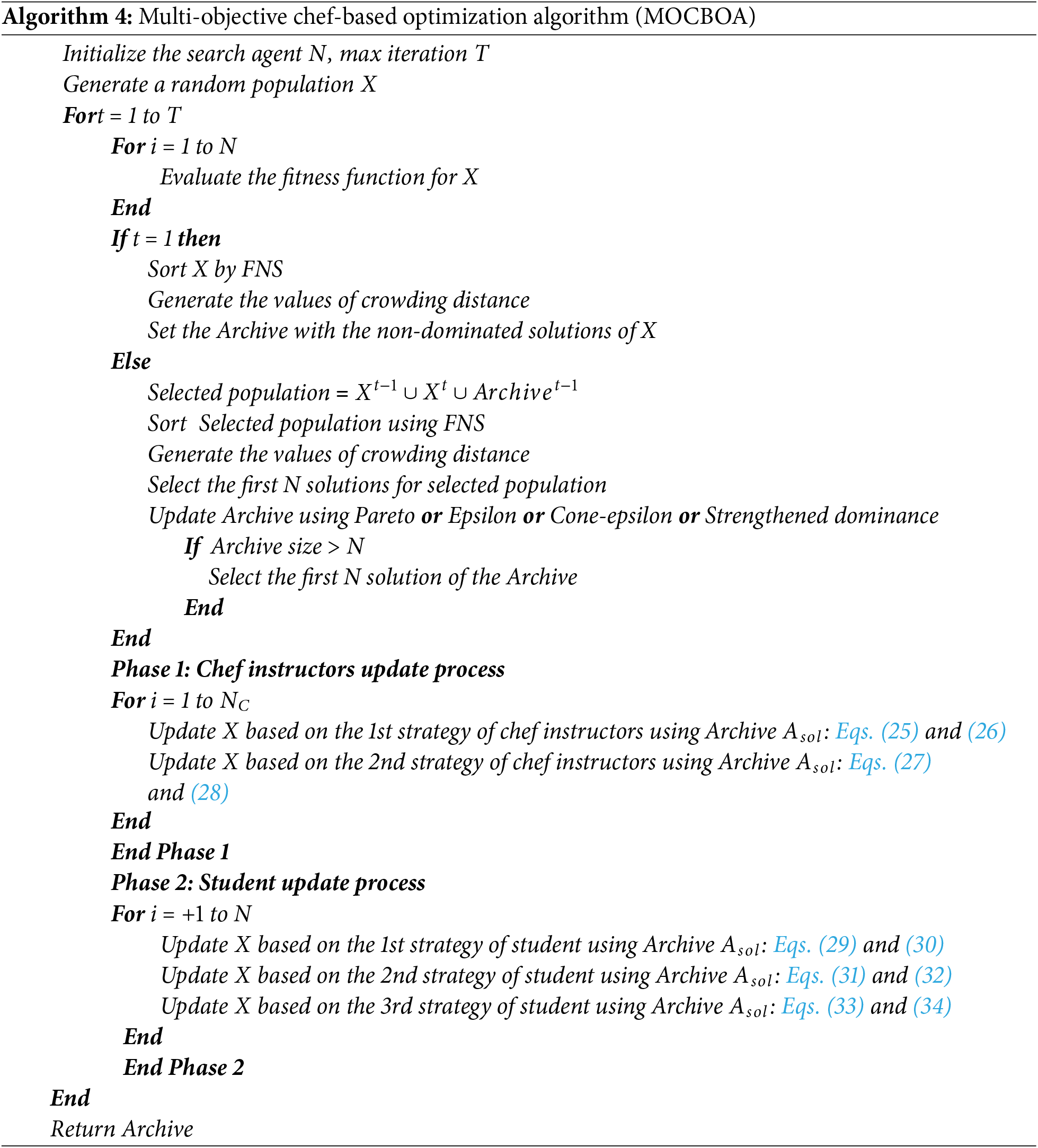
The proposed MOCBOA operates by going through a set of defined steps that are intended to evaluate candidates, systematically explore the solution space, and iteratively refine the population toward optimal solutions. Following establishing the initial population and its evaluation against the M objectives. we began by applying the FNS to the initial population, followed by the crowding distance calculation to identify the most optimal solutions. These top-performing solutions then formed the core of our Selected/Candidate population. After that, we made use of an external archive known as the archive population, which initially contained the first selected population’s non-dominated solution. During every step of the optimization process, this archive kept the best result or the non-dominated set. To achieve Pareto set solutions in every iteration, the algorithm has to carry out the subsequent actions: update the selected population, update the archive population, and then update the population position.

4.1 Selected Population Updating

This population is important since it has a direct impact on the upcoming archive update phase. Its efficacy influences the diversity and quality of the solutions that are kept, which influences the optimization process as a whole. The algorithm iterates through a combined pool of previous, current, and archived populations, selecting the top solutions and systematically evaluating and classifying them to retain the best candidates for further analysis.

•   Create a pool of potential candidates: This pool is created based on combining the previous, current and archive population in order to preserve diversity, maintain a well distributed set of solutions and prevent premature convergence.

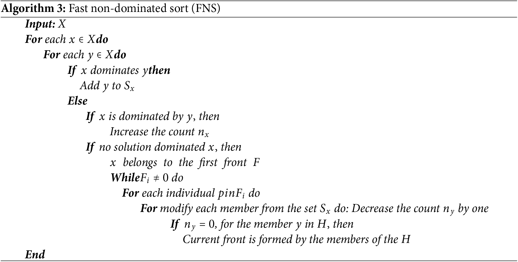
•   Sorting the pool: once the pool is created, the FNS and crowding distance are implemented to sort the solutions accurately according to ranks, after comparing the solutions individually and identifying the non-dominated solutions by checking the two parameters the number of solutions that dominate the solution and the set of solution it dominates. Therefore, if = 0, then those solutions are excluded in a separate front named , after that the whole process is repeated to find the next front solutions.

Algorithm 3 describes the steps adapted by FNS. Once the FNS finishes and to maintain the diversity, the crowding distance is used by calculating for each solution the mean distance to its two surrounding solutions of its cuboid, and ranking them according to this distance. The formulation of the crowding distance is as follows:

(24)

where is the crowding distance of the solution, is the objective function value for the neighboring solutions and of solution The max and min values for the -th objective function are represented by and , respectively, as shown in Fig. 2.

Figure 2: Crowding distance

After calculating the crowding distance of each solution and for each objective function, the solutions are sorted by their crowding distance values that were found in ascending order.

4.2 Archive Updating

The archive population is essential to maintaining the best solutions discovered during the process of optimization. It helps direct the search by influencing subsequent decisions and stores non-dominated solutions to make sure they are not lost. Additionally, the archive preserves diversity by preserving a range of solutions and progresses over time by demonstrating how the quality of solutions increases. It also makes it possible to compare several dominance strategies, including Strengthened dominance, Cone-epsilon dominance, Epsilon dominance, and Pareto dominance. The most optimal and varied set of solutions can be obtained by utilizing one dominant method at a time and examining the archive. Since a clearly defined dominance relation improves convergence, making sure that the optimization process proceeds gradually in the direction of better solutions while maintaining population variety and the search space can be thoroughly explored.

In the update process of the archive, the previously mentioned dominance strategies were used, one at a time. Once the selected population is obtained, it participates in this process by comparing one solution of the archive against the whole selected population. If the archive solution dominates, then it stays in the archive, if not it is replaced by the solution from the selected population. To control the size of the archive and ensure a smooth optimization process, the archive size is limited to the first N solutions.

4.3 Population Updating

Updating the population position to move on with the optimization process is the same as the one employed in the version with only one objective. However, to direct the population towards the Pareto optimal set, the archive population is used in the process. The archive population has been incorporated according to each strategy.

4.3.1 Chef Instructors Update Process

Strategy 1: Modelling themselves after the best chef teacher: This strategy adapts the same equation as the single-objective version using a randomly selected solution of the archive population in the process as follows:

(25)

where this new position is acceptable to the MOCBOA if it dominates as follows:

(26)

Strategy 2: Through individualized exercises and activities: The single-objective version uses a local search and exploitation, with slight adjustments to population members’ positions in the search space, which can yield superior results. This idea states generating a random position around each instructor in the search space. However, since the archive holds the best solutions discovered so far. it is used to help guide the solution towards the optimal results. In the MOCBOA algorithm, instead of generating a local random solution, a random solution is chosen from the archive and used as follows:

(27)

(28)

4.3.2 Students Update Process

Strategy 1: Selecting a random chef and learning a skill: In this strategy, each cooking student selects a class taught by a chef at random, and this chef instructor then teaches cooking techniques. It results in students learning from the best and moving in the search space. In the MOCBOA algorithm, instead of selecting a chef, a solution is selected from the archive as as follows:

(29)

Accordingly, the student’s position is moved, if the new objective function value dominates:

(30)

Strategy 2: Chef selection: One of the variables within the chef is taken to replace by one of the student’s variables. Here, a random variable within a solution from the archive is used as:

(31)

(32)

Strategy 3: Focus on a local search, where students try to improve all of their variables: Using a randomly generated position close by the student, similar to the chef’s second strategy, a new position is generated. As for the MOCBOA algorithm, instead of a random local solution, an archive solution is used as follows:

(33)

(34)

where is a random number from , , &

This process is repeated until the stopping criterion is met. Fig. 3 shows the overall flowchart of the proposed MOCBOA algorithm, and Algorithm 4 describes its pseudo-code.

Figure 3: Flowchart of the proposed MOCBOA algorithm

The computational complexity of the MOCBOA algorithm was analyzed by defining as the population size and as the number of objectives. The main loop of the algorithm shares the same complexity as the CBOA algorithm [25], which operates in polynomial time of , where represents the number of iterations, is the cost function, and is the problem dimension. The first operation, fast non-dominated sorting (FNS), has a complexity of . The second operation, crowding distance calculation, has a complexity of . Updating the archive involves several dominance relations depending on the selected one:

•   Pareto dominance, the most commonly used relation, has a complexity of due to pairwise comparisons of solutions.

•   Epsilon dominance (-dominance), also has a complexity of .

•   Cone--dominance, an extension of -dominance, incurs a complexity of .

•   Strengthened dominance relation, which enhances the selection process by balancing convergence and diversity, typically has a complexity of .

As a result, the overall processing time of GMOEO is determined by the maximum of these complexities: However, the dominant complexity of MOCBOA is , which is consistent with the complexities of MOPSO [8] and MOGWO [9].

5  Results and Discussion

In this section, we validate the proposed algorithm through experiments on real-world engineering problems, known as RWMOPs. These benchmark problems span a variety of engineering and scientific domains, compiled from diverse fields [12]. The test suite includes mechanical design problems (R1–R21), chemical engineering problems (R22–R24), process design and synthesis problems (R25–R29), power electronics problems (R30–R35), and power system problems (R36–R50), in total 50 test cases, as detailed in Table 2.

The main metric used to quantify the performance of the proposed algorithm is the hypervolume indicator (HV) [28] which measures both the convergence and diversity of the solutions, a high HV indicates a better performance. HV evaluates the results of an optimization process by concurrently considering the proximity of points to the Pareto front, as well as diversity and spread. HV also referred to as the measure, represents the volume in the objective space that is dominated by the Pareto front concerning the reference point as a constraint, for all such that . The HV metric is identified as Eq. (35), with as the - Lebesgue measure.

(35)

We assess the effectiveness of four distinct dominance strategies on the performance of the MOCBOA algorithm: Pareto, Epsilon, Cone-epsilon, and Strengthened dominance. For each test problem, we conduct a comprehensive analysis, presenting the best, worst, average, and median outcomes and comparing standard deviations to evaluate the consistency of the solutions. Finally, we examine overall patterns observed across the test problems, comparing the performance of each dominance approach against the others, with a focus on identifying which technique yields the best outcomes in terms of the hypervolume (HV) metric. The experimental settings are standardized to 50 search agents, 10 independent runs, and a maximum of 30,000 function evaluations (i.e., 600 iterations).

5.1 Mechanical Design Problems

Table 3 summarizes the results of MOCBOA across the four dominance techniques to gain a clearer picture of their relative performance on mechanical design problems. Furthermore, Figs. 4 and 5 visually illustrate the performance trends of each dominance technique across the benchmark problems, providing a comparative view of both consistency and variability in results.

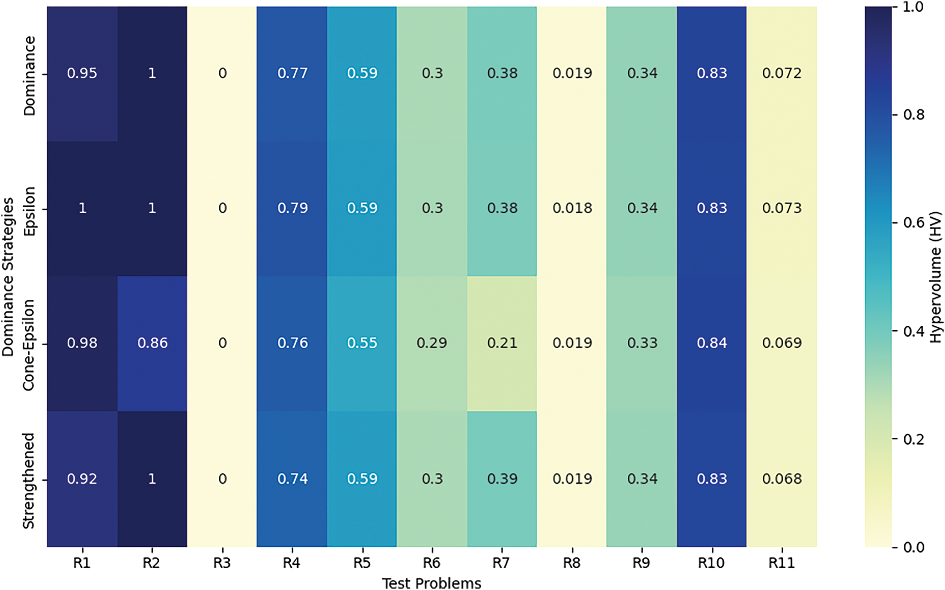
Figure 4: HV analysis across mechanical design problems (R1–R11)

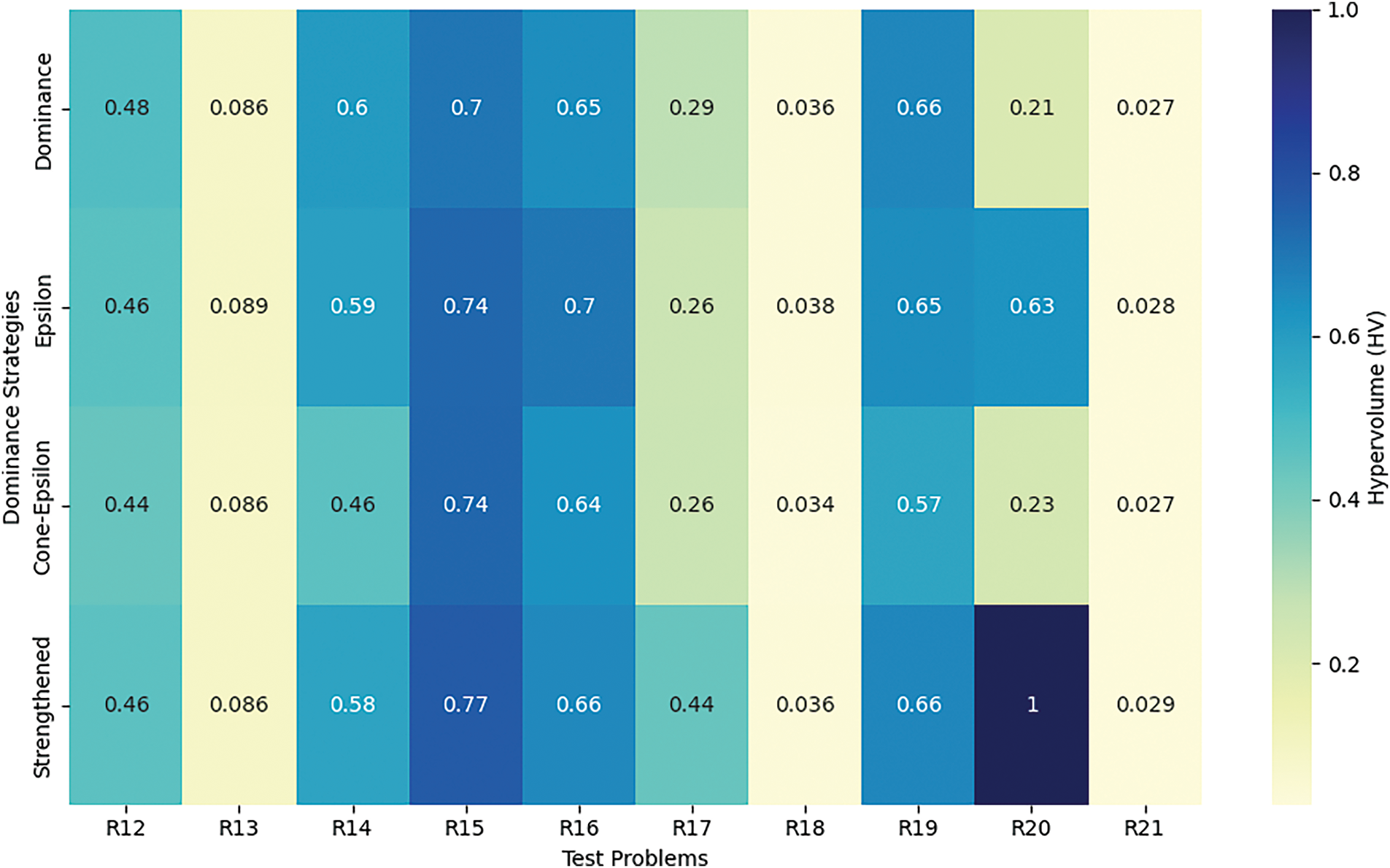
Figure 5: HV analysis across mechanical design problems (R12–R21)

Starting with Pareto dominance, we observe that it consistently achieves respectable median values across the benchmarks, suggesting steady performance. However, it struggles with variability, as indicated by relatively high standard deviations in certain cases, such as in R2 and R7. This variability hints at potential inconsistencies when tackling more intricate problem landscapes. Overall, Pareto dominance demonstrates a solid performance, yet it might be less dependable under more complex conditions. Epsilon dominance, on the other hand, shows stability, particularly with narrow standard deviations in many of the results. For example, its performance on R8 and R16 remains within a tight range, illustrating its ability to handle complex benchmarks consistently. However, its “worst” performance values are generally slightly higher than those observed with Pareto dominance, suggesting that while it maintains reliability, it may sometimes miss achieving the most optimal solutions, possibly due to its tolerance parameter, which affects precision. Moving to Cone-epsilon dominance, this technique seems adept at balancing solution precision and consistency, particularly on benchmarks R9 and R13. It often yields lower best values across several benchmarks, indicating its ability to reach closer-to-optimal solutions in these cases. However, a slight trade-off is apparent, as its median values do not consistently outperform the other techniques. This pattern suggests that while Cone-epsilon is effective at handling specific instances with precision, it may be outperformed in terms of general robustness across varying problem types. Lastly, Strengthened dominance showcases impressive performance on some challenging benchmarks, such as R17 and R18. This technique is especially notable for occasionally achieving exceptionally low “best” values. However, it exhibits considerable variability with broader ranges between best and worst results on some benchmarks. This variability implies that while Strengthened dominance can excel under the right conditions, it may not be as reliable in consistently producing optimal solutions across the board.

The results show that each dominance technique demonstrates unique strengths and weaknesses in addressing the benchmarks. Pareto dominance is solid but somewhat variable, Epsilon dominance is stable yet less precise in finding optimal solutions, Cone-epsilon dominance achieves good precision but has limited general consistency, and Strengthened dominance excels with low best values yet faces variability challenges. These observations underline the importance of selecting the appropriate dominance technique based on specific optimization goals and problem characteristics.

5.2 Chemical Engineering Problems

The results from the MOCBOA algorithm in Table 4 demonstrate clear distinctions in the performance of different dominance approaches across the chemical engineering problems R22–R24. The Epsilon dominance approach consistently delivers stable and high-quality outcomes, showcasing its effectiveness in multi-objective optimization tasks. Its performance is characterized by minimal variability, making it a reliable method for solving complex problems. As shown in Fig. 6, this dominance method performs exceptionally well across all test cases, maintaining consistency even in more challenging scenarios. This consistency underscores the Epsilon dominance approach as a dependable choice when stability is a key requirement in multi-objective optimization.

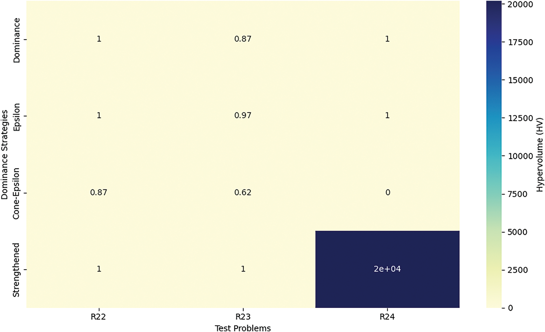
Figure 6: HV analysis across chemical engineering problems (R22–R24)

In contrast, the Dominance approach performs reasonably well in simpler problems but struggles significantly when applied to more complex situations. The results reveal noticeable inconsistencies and variability, particularly in more intricate problems, which make this approach less stable and reliable. These issues suggest that while the Dominance approach may work effectively for straightforward cases, its performance degrades when faced with the added complexity of real-world multi-objective challenges. The variability seen in the results further emphasizes the need for a more robust approach when dealing with difficult problems, making the Dominance approach less suitable for such tasks.

The Cone-epsilon dominance method presents a more nuanced performance. While it shows promising results in certain cases, it also experiences significant variability in others, indicating a high sensitivity to the nature of the problem. This inconsistent behavior suggests that while Cone-epsilon dominance can be effective for some problem types, its performance may not be dependable across the full spectrum of multi-objective optimization problems. Similarly, the Strengthened dominance method demonstrates both strengths and weaknesses. It performs well in some instances but exhibits considerable variability in others, particularly when tackling more challenging problems. According to the obtained results, this approach struggles with stability, particularly in cases where the problem complexity is higher, further emphasizing its unreliability in more difficult scenarios. These findings suggest that the Epsilon dominance approach remains the most stable and reliable choice, while the others may require further refinement or may only be suitable for less complex tasks.

5.3 Process, Design and Synthesis Problems

The results of the MOCBOA algorithm for the process design and synthesis problems (R25–R29) are summarized in Table 5. For the Pareto dominance approach, the results exhibit good consistency in most cases, especially for problems R25, R26, and R29, where the worst, best, and average performance measures show relatively tight ranges. This suggests that Pareto dominance can provide solid solutions in these problems, though there is some variability, particularly with problem R27, which demonstrates a high degree of difficulty as evidenced by the very large worst-case value. This indicates that while Pareto dominance can perform reliably in simpler scenarios, it struggles significantly with more complex problem sets, highlighting its limitations in handling the entire spectrum of multi-objective optimization problems.

The Epsilon dominance approach, on the other hand, shows strong performance in most problems, with notably high average and median values for R25, R26, and R28. The approach excels particularly in its ability to handle the worst-case scenarios, providing a good balance of consistency and quality. However, problems like R27 and R29, especially with the latter having lower performance on average, demonstrate that Epsilon dominance can sometimes struggle with certain problem complexities, leading to a higher standard deviation. This points to a method that is highly effective in many cases but still sensitive to the specific nature of the problem, requiring further refinement or adjustments to handle outliers effectively.

The Cone-epsilon dominance approach exhibits a mixed performance across the problem set, with some issues like R27 and R29 showing significant variability and poor results. The worst-case values for R27 in particular are quite high, signaling that this approach may not be the best choice for all types of optimization problems. The results reveal that while Cone-epsilon dominance can be effective in simpler cases like R25 and R26, it struggles significantly in more complicated scenarios, as seen in R27. Similarly, the Strengthened dominance approach presents a contrasting performance, with some very large worst-case values for problems like R25 and R27, but it also provides some strong results, particularly for R28 and R29. This shows that the Strengthened dominance method can excel in some areas but has considerable instability, especially for more complex problems. As illustrated in Fig. 7, these variations in the performance across different dominance methods reinforce the need for a careful selection of the right approach depending on the problem’s characteristics and complexity.

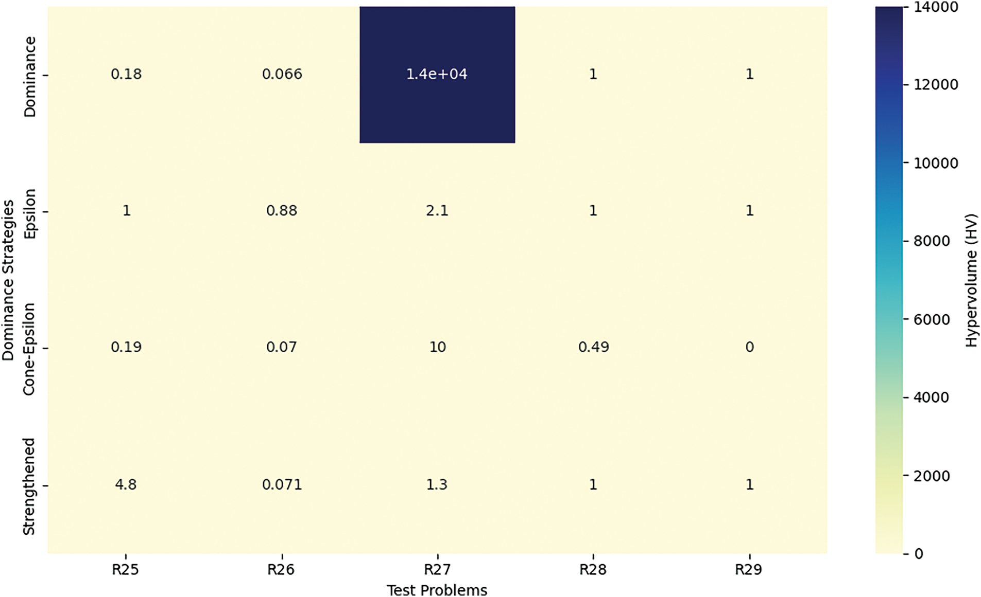
Figure 7: HV analysis across process, design and synthesis problems (R25–R29)

5.4 Power Electronics Problems

The results of the MOCBOA algorithm applied to power electronics problems (R30–R35) in Table 6 reveal interesting patterns across the various dominance approaches. The obtained results in this section can be discussed as follows:

When examining the Pareto dominance results, we see a considerable variation in the performance across the different problems. The worst-case performance for R31 and R35 stands out, with values much higher than for other problems, especially in the case of R35, where the worst-case performance reaches nearly 1. This suggests that Pareto’s dominance faces significant challenges when dealing with these specific power electronics problems, likely due to their complexity. On the other hand, the best-case results for problems like R30, R32, and R34 show promising outcomes, indicating that the algorithm can sometimes find near-optimal solutions under favorable conditions. The median and average values further illustrate a consistent ability to find good solutions, with some issues (R33, R35) showing high average performance despite the large worst-case values.

The Epsilon dominance approach generally follows a similar trend, where problems like R30 and R35 exhibit high worst-case values, indicating challenges in finding optimal solutions. However, this approach performs quite well in terms of average performance, with the average values across most problems (e.g., R30, R31, R33) showing promising results. Notably, the standard deviations are generally higher compared to the Pareto dominance approach, especially for problems R30 and R31, suggesting that Epsilon dominance is more sensitive to problem complexities and may struggle with certain problem instances. Nevertheless, it still demonstrates the potential for high-quality solutions in many cases, particularly for problems where the best values are zero, indicating that the algorithm can achieve optimal or near-optimal results.

The Cone-epsilon dominance approach, which generally shows lower worst-case values, particularly for problems R30 to R34, tends to offer more stability. However, the average and median values for many of the problems (such as R30, R32, and R34) are consistently zero, which indicates that the approach is unable to generate diverse solutions and may fail to address the full range of objectives in these problems. For more complex problems like R35, Cone-epsilon dominance performs relatively better, although the performance still falls short compared to other approaches.

Lastly, the Strengthened dominance approach presents mixed results. While the worst-case values are high for most problems (particularly for R30, R31, and R35), the best-case results indicate that Strengthened dominance can find optimal solutions under certain conditions. This method tends to generate solid performance in terms of average values, though the variability is high, as evidenced by the large standard deviations for most problems.

Overall, while each dominance approach shows its strengths, the results indicate that selecting the most appropriate method depends heavily on the specific characteristics of the power electronics problems at hand. The HV analysis, as shown in Fig. 8, further highlights the differences in the performance across these approaches, suggesting that a hybrid or adaptive strategy might be beneficial to optimize the results for complex problem sets.

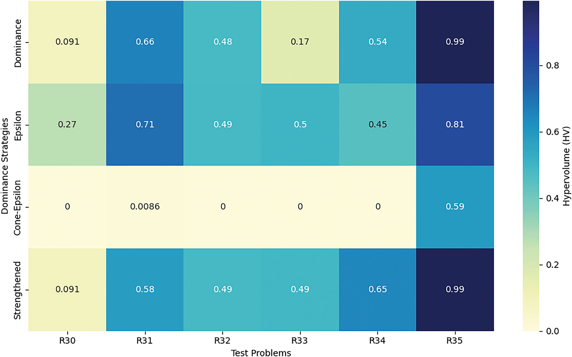
Figure 8: HV analysis across power electronics problems (R30–R35)

5.5 Power System Problems

In this section, we present an analysis and discussion of the results from Table 7, which shows the performance of the MOCBOA algorithm across different power system problems (R36–R50). The table includes metrics based on four dominance techniques: Pareto, Epsilon, Cone-epsilon, and Strengthened dominance. To visualize and further interpret these results, Figs. 9 and 10 depict the HV analysis across the problems R36–R43 and R44–R50, respectively.

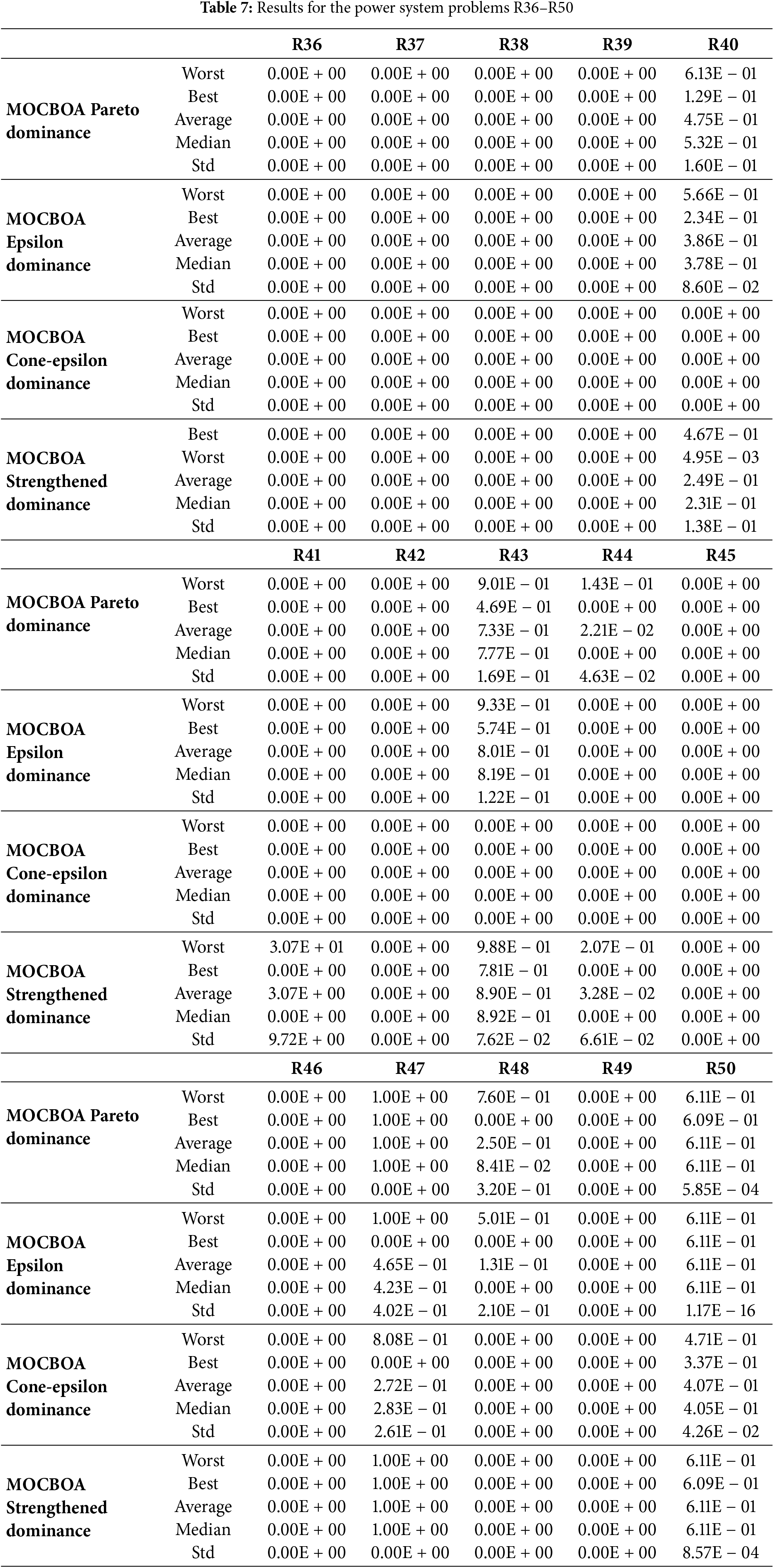
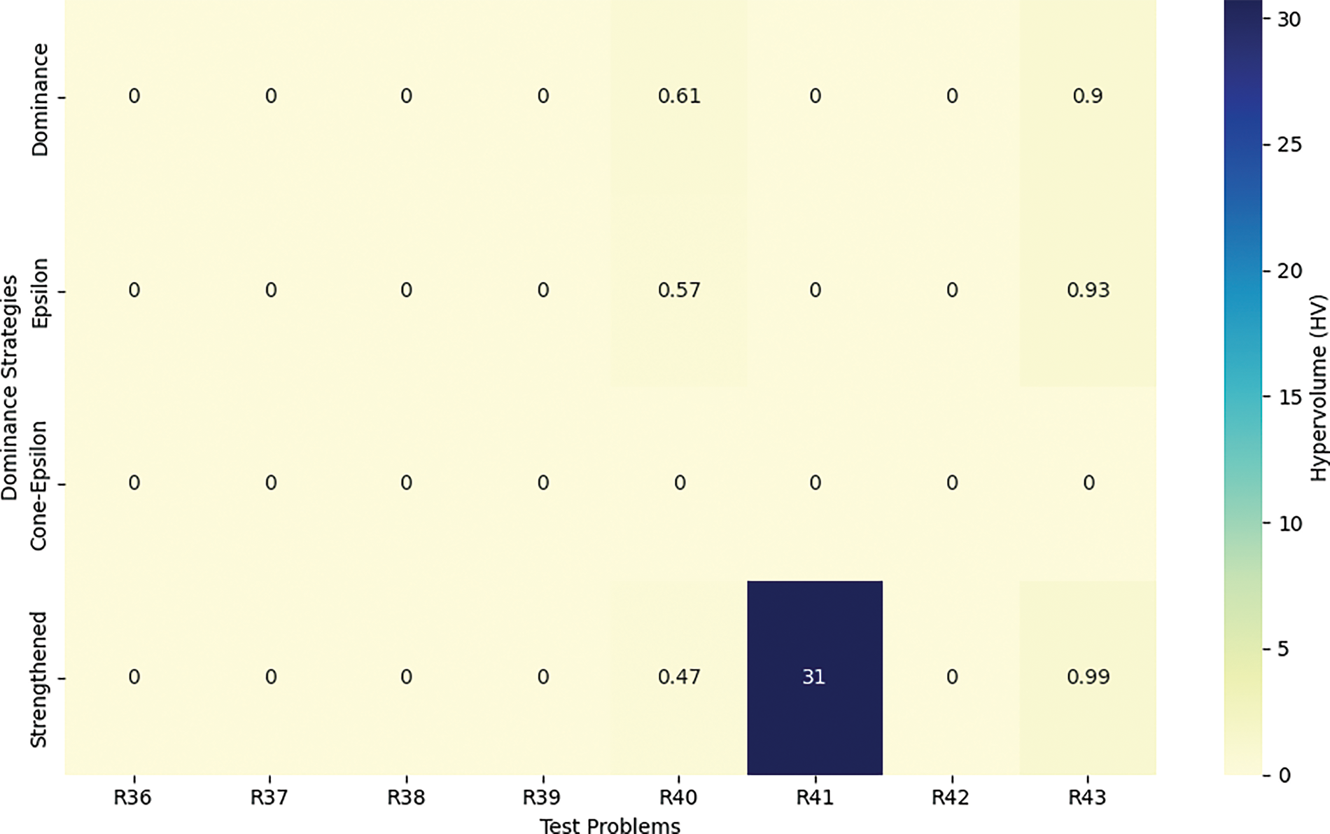
Figure 9: HV analysis across power systems problems (R36–R43)

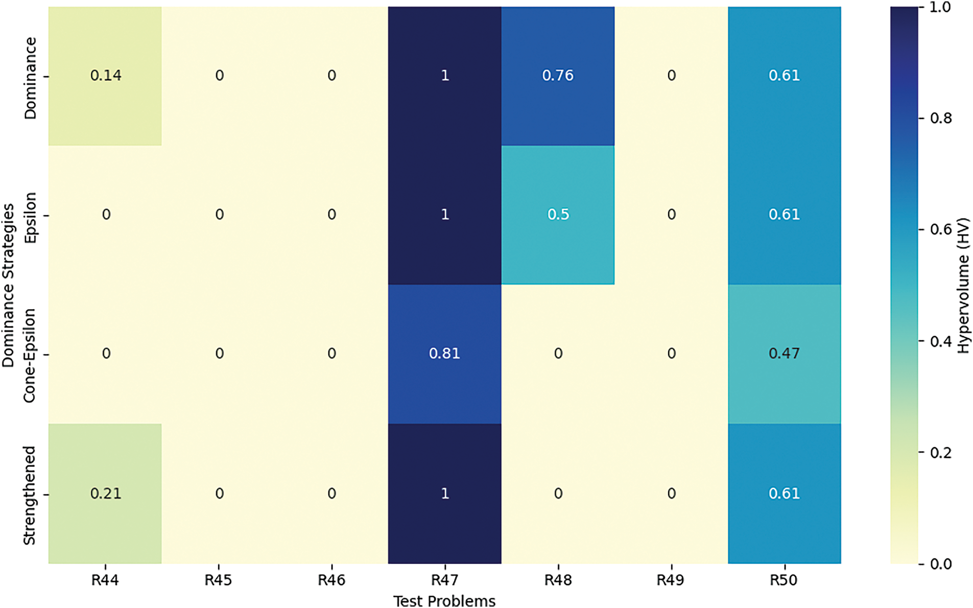
Figure 10: HV analysis across power systems problems (R44–R50)

From Table 7, it is clear that the MOCBOA algorithm consistently yields a “Worst” value of 0.00E + 00 across the majority of the problems under the Pareto and Epsilon dominance techniques, which indicates that the algorithm performs well in avoiding poor solutions. However, the “Best” values vary more noticeably, especially for problems R39–R42, where the results are non-zero, showing that the algorithm reaches better solutions in these cases. The “Average” values for all problems are generally low, confirming the robustness of the algorithm in maintaining a high-quality solution across different instances. The standard deviation (Std) remains very small, which further supports the consistency of MOCBOA across all problems.

In contrast, under the Cone-epsilon dominance technique, all the metrics for the worst, best, average, median, and standard deviation are zero, indicating that this technique may not have contributed positively to the solution diversity or quality in this particular case. The Strengthened dominance technique, however, shows more variation in the results. For the problems R41–R43, the “Worst” value appears to be considerably high (e.g., 3.07E + 01 for R41), but it still manages to show a “Best” solution around 7.81E − 01 for R43, which suggests that the Strengthened dominance technique might handle specific power system challenges more effectively.

Fig. 9 and 10 complement these findings by presenting the HV analysis for the power system problems R36–R43 and R44–R50, respectively. In Fig. 9, the HV values are generally high for most problems, suggesting that the MOCBOA algorithm performs well in both converging to optimal solutions and maintaining diversity in its solutions. Problems R40 and R42 exhibit slightly lower HV values, indicating a possible area for improvement. On the other hand, in Fig. 10, the HV values remain consistently high, with a noticeable peak in R45, showing that the algorithm achieves an optimal convergence in these problems. This analysis demonstrates that MOCBOA excels in solving complex multi-objective optimization problems in power systems, particularly for problems R44–R50, where the HV values indicate an effective balance between convergence and diversity.

Overall, the results indicate that MOCBOA’s performance varies across different power system problems, with significant improvement in convergence and diversity for specific problem instances. The Pareto and Epsilon dominance techniques generally yield good results, while the Strengthened dominance method shows potential for specific problem sets.

5.6 Comparison

Table 8 describes standard parameter settings for each of the algorithms utilized in this experiment: MOGSK, MOEA/D, NSGAII, and SPEA2. Adopting these generally accepted parameters from the literature assures a fair and unbiased comparison by reducing the potential impact of parameter adjustment on the performance outcomes. This method enables us to focus on the inherent strengths and shortcomings of each algorithm under consistent conditions.

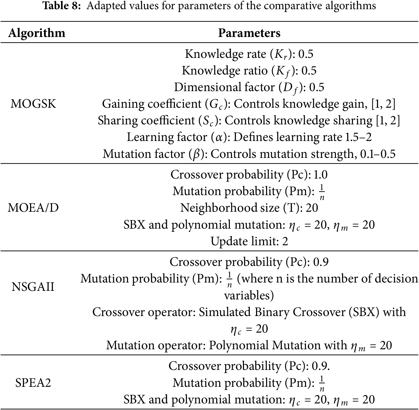
Table 9 presents a comprehensive performance comparison between the proposed MOCBOA algorithm and the existing MOGSK algorithm [14], NSGAII [5], MOEA/D [7], and SPEA2 [6], across 50 test problems (R1–R50), using Hyper volume as the evaluation metric. Fig. 11 provides a visual comparison of the average performance across all test problems. We note that the PlatEmov [67] was used to generate the results for the algorithms NSGAII, MOEA/D, and SPEA2.

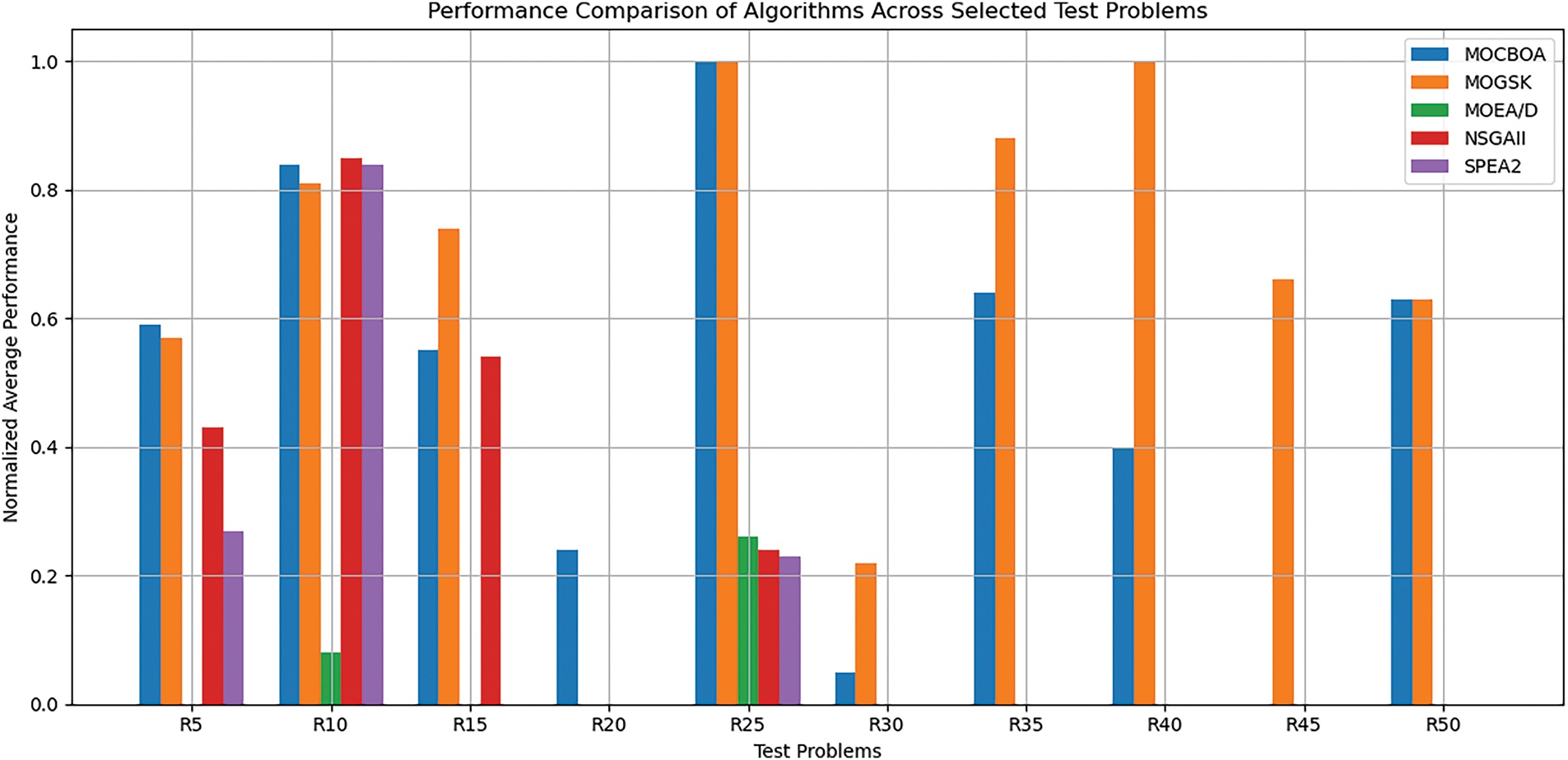
Figure 11: Comparing the proposed MOCBOA algorithm with the MOGSK, NSGAII, MOEA/D and SPEA2 algorithms, on average across selected test problems from R1–R50

Across multiple test problems, MOGSK generally achieves higher and more stable Hypervolume values than MOCBOA. However, MOCBOA occasionally outperforms MOGSK in certain instances, particularly in the best values. For example, in R2, MOCBOA achieves 7.40E − 01, outperforming MOGSK’s 3.80E − 01. However, MOGSK performs better in many other test cases, such as R1 (9.92E − 01) and R22 (9.82E − 01), where it surpasses MOCBOA.

Stability-wise, MOGSK tends to exhibit lower standard deviations in many cases, indicating a more consistent performance. Although MOCBOA has competitive results in some problems, it displays more variability across the test problems, leading to higher standard deviations in multiple cases.

Regarding MOEA/D, the results indicate a large number of NaN values, meaning it fails to converge in multiple instances. When MOEA/D does produce results, its Hypervolume values are generally lower than those of MOGSK and MOCBOA. For example, in R25, MOEA/D records 4.00E − 01, whereas MOCBOA achieves 8.64E − 01. However, in R7, MOEA/D (4.79E − 01) performs better than MOCBOA (0.00E + 00).

NSGA-II performs competitively in certain cases but is inconsistent overall. For example, in R1, MOCBOA records 9.92E − 01, while NSGA-II only reaches 5.96E − 01. However, in R27, NSGA-II shows an extremely high best value (1.80E + 11), which might be an anomaly. Additionally, NSGA-II often exhibits higher standard deviations, suggesting a less stable performance compared to MOGSK and MOCBOA.

SPEA2 also suffers from convergence issues, as indicated by many NaN values across the test cases. However, when valid results exist, MOCBOA often outperforms SPEA2. For instance, in R5, MOCBOA achieves 4.89E − 01, while SPEA2 only records 2.77E − 01. This means that SPEA2 performs better than MOCBOA in R7 (4.83E − 01 vs. 0.00E + 00).

The MOCBOA algorithm’s competitive advantage in multi-objective optimization is demonstrated by its performance on a variety of test problems. It continuously performs better than a number of benchmark algorithms, including SPEA2, NSGA-II, and MOEA/D, particularly when it comes to the optimum Hypervolume values. In many cases, MOCBOA performs exceptionally well, demonstrating excellent solution quality and continuously attaining better average Hypervolume outcomes, which suggests its capacity to efficiently explore the solution space. Even though MOCBOA typically outperforms MOGSK, it can occasionally have problems with stability, as evidenced by greater standard deviations, which point to less reliable performance. Despite this, MOCBOA frequently exhibits superior convergence and dependable outcomes in contrast to MOEA/D and SPEA2, which have several NaN values as a result of convergence problems. Although MOCBOA performs exceptionally well in many problem contexts, it occasionally falls behind MOGSK, which exhibits a superior stability and solution quality. However, MOCBOA is an excellent candidate for multi-objective optimization tasks due to its ability to handle a variety of optimization problems and consistently produce competitive results. This is especially true when paired with upcoming enhancements to improve stability and robustness across all test cases.

6  Conclusions

In this paper, we have proposed a multi-objective optimization algorithm, MOCBOA, which extends the recently introduced CBOA algorithm. The MOCBOA has been designed by incorporating several effective strategies to enhance its performance. Specifically, it utilizes fast non-dominated sorting and crowding distance measures to control the distribution and diversity of solutions during both the exploitation and exploration phases of the optimization process. Additionally, an external repository has been employed to store the best solutions, which serves to guide the population towards the optimal Pareto front. The archive of solutions has been updated using various dominance relations. The effectiveness of the proposed MOCBOA algorithm has been tested on a comprehensive set of benchmarks, which were sourced from various domains, including mechanical design, chemical engineering, power electronics, process design and synthesis, and power system optimization. The comparative results of MOCBOA’s performance in problems such as R2 and R27 with Hypervolume values of 0.740 and 1.65, along with its capacity to produce dependable and consistent outcomes in situations when some competitors stumble (such as when they run across NaN values), show that it is a robust and competitive strategy, particularly in terms of solution quality, stability, and convergence speed. Since multi-objective optimization is the foundation of our approach, its usefulness goes well beyond the scope of the current study. Because MOCBOA may simultaneously optimize conflicting objectives, it is especially well-suited to solving complicated problems across a variety of fields.

Despite the promising performance of the MOCBOA algorithm, there are a few limitations that need further investigation. First, although Epsilon dominance has proven to be effective, the algorithm’s performance might vary for certain types of problems, particularly those with a complex Pareto front. In such cases, the trade-off between exploration and exploitation may need further tuning. Additionally, the computational cost of maintaining and updating the external repository with multiple dominance relations could increase with larger problem instances, affecting the algorithm’s scalability. Therefore, future work should focus on improving the algorithm’s efficiency for large-scale problems by managing the external repository and reducing the computational burden. Further experiments on a wider range of problem domains, particularly those with non-convex or discontinuous Pareto fronts, would also provide valuable insights into the robustness of MOCBOA. Also, hybridizing MOCBOA with knowledge-based heuristics, fuzzy systems, and machine learning techniques could be explored to further enhance its performance in dynamic and real-time optimization scenarios.

Acknowledgement: The authors present their appreciation to King Saud University for funding the publication of this research through Researchers Supporting Program (RSPD2024R809), King Saud University, Riyadh, Saudi Arabia.

Funding Statement: The research is funded by Researchers Supporting Program number (RSPD2024R809), King Saud University, Riyadh, Saudi Arabia.

Author Contributions: Nour Elhouda Chalabi: Conceptualization, resources, methodology, data curation, experimental design, software implementation, writing—original draft preparation. Abdelouahab Attia: Methodology, data collection, software implementation, validation, visualization, writing—review and editing. Abdulaziz S. Almazyad: Project administration, funding acquisition, validation, formal analysis, writing—review and editing. Ali Wagdy Mohamed: Methodology, validation, formal analysis, writing—review and editing. Frank Werner: Supervision, validation, formal analysis, writing—review and editing. Pradeep Jangir: Methodology, visualization, writing—original draft preparation. Mohammad Shokouhifar: Supervision, formal analysis, writing—review and editing. All authors reviewed the results and approved the final version of the manuscript.

Availability of Data and Materials: Data sharing not applicable to this article as no datasets were generated or analyzed during the current study.

Ethics Approval: Not applicable.

Conflicts of Interest: The authors declare no conflicts of interest to report regarding the present study.

References

1. Wang WC, Tian WC, Xu DM, Zang HF. Arctic puffin optimization: a bio-inspired metaheuristic algorithm for solving engineering design optimization. Adv Eng Softw. 2024;195:103694. doi:10.1016/j.advengsoft.2024.103694. [Google Scholar] [CrossRef]

2. Wang WC, Xu L, Chau KW, Zhao Y, Xu DM. An orthogonal opposition-based-learning Yin-Yang-pair optimization algorithm for engineering optimization. Eng Comput. 2022;38(2):1149–83. doi:10.1007/s00366-020-01248-9. [Google Scholar] [CrossRef]

3. Al Mindeel T, Spentzou E, Eftekhari M. Energy, thermal comfort, and indoor air quality: multi-objective optimization review. Renew Sustain Energy Rev. 2024;202(11):114682. doi:10.1016/j.rser.2024.114682. [Google Scholar] [CrossRef]

4. Han Z, Han W, Ye Y, Sui J. Multi-objective sustainability optimization of a solar-based integrated energy system. Renew Sustain Energy Rev. 2024;202(4):114679. doi:10.1016/j.rser.2024.114679. [Google Scholar] [CrossRef]

5. Deb K, Pratap A, Agarwal S, Meyarivan T. A fast and elitist multiobjective genetic algorithm: NSGA-II. IEEE Trans Evol Comput. 2002;6(2):182–97. doi:10.1109/4235.996017. [Google Scholar] [CrossRef]

6. Zitzler E, Laumanns M, Thiele L. SPEA2: improving the strength Pareto evolutionary algorithm. In: TIK report 103. Zurich, Switzerland: ETH Zurich; 2001. [Google Scholar]

7. Zhang Q, Li H. MOEA/D: a multiobjective evolutionary algorithm based on decomposition. IEEE Trans Evol Comput. 2007;11(6):712–31. doi:10.1109/TEVC.2007.892759. [Google Scholar] [CrossRef]

8. Coello Coello CA, Reyes-Sierra M. Multi-objective particle swarm optimizers: a survey of the state-of-the-art. Int J Comput Intell Res. 2006;2(3):287–308. doi:10.5019/j.ijcir.2006.68. [Google Scholar] [CrossRef]

9. Mirjalili S, Saremi S, Mirjalili SM, Coelho LDS. Multi-objective grey wolf optimizer: a novel algorithm for multi-criterion optimization. Expert Syst Appl. 2016;47(6):106–19. doi:10.1016/j.eswa.2015.10.039. [Google Scholar] [CrossRef]

10. Pradhan PM, Panda G. Solving multiobjective problems using cat swarm optimization. Expert Syst Appl. 2012;39(3):2956–64. doi:10.1016/j.eswa.2011.08.157. [Google Scholar] [CrossRef]

11. Patil MV, Kulkarni AJ. Pareto dominance based multiobjective cohort intelligence algorithm. Inf Sci. 2020;538(1):69–118. doi:10.1016/j.ins.2020.05.019. [Google Scholar] [CrossRef]

12. Chalabi NE, Attia A, Bouziane A, Hassaballah M, Alanazi A, Binbusayyis A. An archive-guided equilibrium optimizer based on Epsilon dominance for multi-objective optimization problems. Mathematics. 2023;11(12):2680. doi:10.3390/math11122680. [Google Scholar] [CrossRef]

13. Chalabi NE, Attia A, Bouziane A, Hassaballah M. An improved marine predator algorithm based on Epsilon dominance and Pareto archive for multi-objective optimization. Eng Appl Artif Intell. 2023;119(1):105718. doi:10.1016/j.engappai.2022.105718. [Google Scholar] [CrossRef]

14. Chalabi NE, Attia A, Alnowibet KA, Zawbaa HM, Masri H, Mohamed AW. A multi-objective gaining-sharing knowledge-based optimization algorithm for solving engineering problems. Mathematics. 2023;11(14):3092. doi:10.3390/math11143092. [Google Scholar] [CrossRef]

15. Menchaca-Méndez A, Montero E, Antonio LM, Zapotecas-Martínez S, Coello Coello CA, Riff MC. A co-evolutionary scheme for multi-objective evolutionary algorithms based on ϵ—dominance. IEEE Access. 2019;7:18267–83. doi:10.1109/ACCESS.2019.2896962. [Google Scholar] [CrossRef]

16. Li H, Deng J, Zhang Q, Sun J. Adaptive Epsilon dominance in decomposition-based multiobjective evolutionary algorithm. Swarm Evol Comput. 2019;45(1):52–67. doi:10.1016/j.swevo.2018.12.007. [Google Scholar] [CrossRef]

17. Zouache D, Ben Abdelaziz F. Guided Manta Ray foraging optimization using Epsilon dominance for multi-objective optimization in engineering design. Expert Syst Appl. 2022;189(1):116126. doi:10.1016/j.eswa.2021.116126. [Google Scholar] [CrossRef]

18. Deutz AH, Emmerich M, Wang Y. Many-criteria dominance relations. In: Brockhoff D, Emmerich M, Naujoks B, Purshouse R, editors. Many-criteria optimization and decision analysis. Natural computing series. Cham, Switzerland: Springer Cham; 2023. p. 81–111. [Google Scholar]

19. Batista LS, Campelo F, Guimaraes FG, Ramírez JA. Pareto cone ε-dominance: improving convergence and diversity in multiobjective evolutionary algorithms. In: Evolutionary Multi-Criterion Optimization: 6th International Conference, EMO 2011; 2011; Ouro Preto, Brazil. p. 76–90. [Google Scholar]

20. Zouache D, Got A, Drias H. An external archive guided Harris Hawks optimization using strengthened dominance relation for multi-objective optimization problems. Artif Intell Rev. 2023;56(3):2607–38. doi:10.1007/s10462-022-10235-z. [Google Scholar] [CrossRef]

21. Shen J, Wang P, Wang X. A controlled strengthened dominance relation for evolutionary many-objective optimization. IEEE Trans Cybern. 2022;52(5):3645–57. doi:10.1109/TCYB.2020.3015998. [Google Scholar] [PubMed] [CrossRef]

22. Gu Q, Chen H, Chen L, Li X, Xiong NN. A many-objective evolutionary algorithm with reference points-based strengthened dominance relation. Inf Sci. 2021;554:236–55. doi:10.1016/j.ins.2020.12.025. [Google Scholar] [CrossRef]

23. Zouache D, Ben Abdelaziz F. MGDE: a many-objective guided differential evolution with strengthened dominance relation and bi-goal evolution. Ann Oper Res. 2022;19(1):45. doi:10.1007/s10479-022-04641-3. [Google Scholar] [CrossRef]

24. Laumanns M, Thiele L, Deb K, Zitzler E. Combining convergence and diversity in evolutionary multiobjective optimization. Evol Comput. 2002;10(3):263–82. doi:10.1162/106365602760234108. [Google Scholar] [PubMed] [CrossRef]

25. Trojovská E, Dehghani M. A new human-based metahurestic optimization method based on mimicking cooking training. Sci Rep. 2022;12(1):14861. doi:10.1038/s41598-022-19313-2. [Google Scholar] [PubMed] [CrossRef]

26. Ikeda K, Kita H, Kobayashi S. Failure of Pareto-based MOEAs: does non-dominated really mean near to optimal?. In: Proceedings of the 2001 Congress on Evolutionary Computation; 2001 May 27–30; Seoul, Republic of Korea: IEEE; 2002. p. 957–62. doi:10.1109/CEC.2001.934293. [Google Scholar] [CrossRef]

27. Tian Y, Cheng R, Zhang X, Su Y, Jin Y. A strengthened dominance relation considering convergence and diversity for evolutionary many-objective optimization. IEEE Trans Evol Comput. 2019;23(2):331–45. doi:10.1109/TEVC.2018.2866854. [Google Scholar] [CrossRef]

28. Chao T, Wang S, Wang S, Yang M. A many-objective evolutionary algorithm combining simplified hypervolume and a method for reference point sampling based on angular relationship. Appl Soft Comput. 2024;163(3):111881. doi:10.1016/j.asoc.2024.111881. [Google Scholar] [CrossRef]

29. Kannan BK, Kramer SN. An augmented Lagrange multiplier based method for mixed integer discrete continuous optimization and its applications to mechanical design. In: ASME 1993 Design Technical Conferences; 1993 Sep 19–22; Albuquerque, NM, USA; 2021. p. 103–12. doi:10.1115/DETC1993-0382. [Google Scholar] [CrossRef]

30. Narayanan S, Azarm S. On improving multiobjective genetic algorithms for design optimization. Struct Optim. 1999;18(2):146. doi:10.1007/BF01195989. [Google Scholar] [CrossRef]

31. Chiandussi G, Codegone M, Ferrero S, Varesio FE. Comparison of multi-objective optimization methodologies for engineering applications. Comput Mathem Applicat. 2012;63(5):912–42. doi:10.1016/j.camwa.2011.11.057. [Google Scholar] [CrossRef]

32. Deb K. Evolutionary algorithms for in engineering design. Evolution Algor Engd Comput Sci. 1999;2:135–61. [Google Scholar]

33. Osyczka A, Kundu S. A genetic algorithm-based multicriteria optimization method. In: The First World Congress of Structural and Multidisciplinary Optimization;1995 Goslar, Germany; p.909–14. [Google Scholar]

34. Azarm S, Tits A, Fan M. Tradeoff-driven optimization-based design of mechanical systems. In: 4th Symposium on Multidisciplinary Analysis and Optimization; 1992; USA. 4758 p. doi:10.2514/6.1992-4758. [Google Scholar] [CrossRef]

35. Ray T, Liew KM. A swarm metaphor for multiobjective design optimization. Eng Optim. 2002;34(2):141–53. doi:10.1080/03052150210915. [Google Scholar] [CrossRef]

36. Deb K, Jain H. An evolutionary many-objective optimization algorithm using reference-point-based nondominated sorting approach, part I: solving problems with box constraints. IEEE Trans Evol Comput. 2013;18(4):577–601. doi:10.1109/TEVC.2013.2281535. [Google Scholar] [CrossRef]

37. Cheng FY, Li XS. Generalized center method for multiobjective engineering optimization. Eng Optim. 1999;31(5):641–61. doi:10.1080/03052159908941390. [Google Scholar] [CrossRef]

38. Huang HZ, Gu YK, Du X. An interactive fuzzy multi-objective optimization method for engineering design. Eng Appl Artif Intell. 2006;19(5):451–60. doi:10.1016/j.engappai.2005.12.001. [Google Scholar] [CrossRef]

39. Steven G. Evolutionary algorithms for single and multicriteria design optimization. A. Osyczka. Springer Verlag, Berlin, 2002, ISBN 3-7908-1418-01. Struct Multidiscip Optim. 2002;24:88–9. doi:10.1007/s00158-002-0218-y. [Google Scholar] [CrossRef]

40. Coello C, Lamont G, Veldhuizen DV. Evolutionary algorithms for solving multi-objective problems. In: Genetic and evolutionary computation series. 2nd ed. New York, NY, USA: Springer; 2007. [Google Scholar]

41. Parsons MG, Scott RL. Formulation of multicriterion design optimization problems for solution with scalar numerical optimization methods. J Ship Res. 2004;48(1):61–76. doi:10.5957/jsr.2004.48.1.61. [Google Scholar] [CrossRef]

42. Fan L, Yoshino T, Xu T, Lin Y, Liu H. A novel hybrid algorithm for solving multiobjective optimization problems with engineering applications. Math Probl Eng. 2018;2018:5316379. doi:10.1155/2018/5316379. [Google Scholar] [CrossRef]

43. Dhiman G, Kumar V. Multi-objective spotted hyena optimizer: a Multi-objective optimization algorithm for engineering problems. Knowl Based Syst. 2018;150(6):175–97. doi:10.1016/j.knosys.2018.03.011. [Google Scholar] [CrossRef]

44. Mahon K. Optimal engineering design: principles and applications (mechanical engineering series, volume 14). J Oper Res Soc. 1983;34(7):652–4. doi:10.1057/jors.1983.155. [Google Scholar] [CrossRef]

45. Zhang H, Peng Y, Hou L, Tian G, Li Z. A hybrid multi-objective optimization approach for energy-absorbing structures in train collisions. Inf Sci. 2019;481(4):491–506. doi:10.1016/j.ins.2018.12.071. [Google Scholar] [CrossRef]

46. Floudas CA, Pardalos PM. A collection of test problems for constrained global optimization algorithms. Berlin/Heidelberg, Germany: Springer; 1990. [Google Scholar]

47. Ryoo HS, Sahinidis NV. Global optimization of nonconvex NLPs and MINLPs with applications in process design. Comput Chem Eng. 1995;19(5):551–66. doi:10.1016/0098-1354(94)00097-2. [Google Scholar] [CrossRef]

48. Guillén-Gosálbez G. A novel MILP-based objective reduction method for multi-objective optimization: application to environmental problems. Comput Chem Eng. 2011;35(8):1469–77. doi:10.1016/j.compchemeng.2011.02.001. [Google Scholar] [CrossRef]

49. Kocis GR, Grossmann IE. A modelling and decomposition strategy for the minlp optimization of process flowsheets. Comput Chem Eng. 1989;13(7):797–819. doi:10.1016/0098-1354(89)85053-7. [Google Scholar] [CrossRef]

50. Kocis GR, Grossmann IE. Global optimization of nonconvex mixed-integer nonlinear programming (MINLP) problems in process synthesis. Ind Eng Chem Res. 1988;27(8):1407–21. doi:10.1021/ie00080a013. [Google Scholar] [CrossRef]

51. Floudas CA. Nonlinear and mixed-integer optimization: fundamentals and applications. New York, NY, USA: Oxford University Press; 1995. [Google Scholar]

52. Rathore AK, Holtz J, Boller T. Synchronous optimal pulsewidth modulation for low-switching-frequency control of medium-voltage multilevel inverters. IEEE Trans Ind Electron. 2010;57(7):2374–81. doi:10.1109/TIE.2010.2047824. [Google Scholar] [CrossRef]

53. Rathore AK, Holtz J, Boller T. Optimal pulsewidth modulation of multilevel inverters for low switching frequency control of medium voltage high power industrial AC drives. In: 2010 IEEE Energy Conversion Congress and Exposition; 2010 Sep 12–16; Atlanta, GA, USA: IEEE; 2010. p. 4569–74. doi:10.1109/ECCE.2010.5618413. [Google Scholar] [CrossRef]

54. Edpuganti A, Rathore AK. Fundamental switching frequency optimal pulsewidth modulation of medium-voltage cascaded seven-level inverter. IEEE Trans Ind Appl. 2015;51(4):3485–92. doi:10.1109/TIA.2015.2394485. [Google Scholar] [CrossRef]

55. Edpuganti A, Dwivedi A, Rathore AK, Srivastava RK. Optimal pulsewidth modulation of cascade nine-level (9L) inverter for medium voltage high power industrial AC drives. In: IECON 2015-41st Annual Conference of the IEEE Industrial Electronics Society; 2015 Nov 9–12; Yokohama, Japan: IEEE; 2015. p. 4259–64. doi:10.1109/IECON.2015.7392764. [Google Scholar] [CrossRef]

56. Edpuganti A, Rathore AK. Optimal pulsewidth modulation for common-mode voltage elimination scheme of medium-voltage modular multilevel converter-fed open-end stator winding induction motor drives. IEEE Trans Ind Electron. 2017;64(1):848–56. doi:10.1109/TIE.2016.2586678. [Google Scholar] [CrossRef]

57. Mishra S, Kumar A, Singh D, Kumar Misra R. Butterfly optimizer for placement and sizing of distributed generation for feeder phase balancing. Adv Intell Syst Comput. 2019;799:519–30. [Google Scholar]

58. Biswas PP, Suganthan PN, Mallipeddi R, Amaratunga GAJ. Multi-objective optimal power flow solutions using a constraint handling technique of evolutionary algorithms. Soft Comput. 2020;24(4):2999–3023. doi:10.1007/s00500-019-04077-1. [Google Scholar] [CrossRef]

59. Kumar A, Das S, Mallipeddi R. An inversion-free robust power-flow algorithm for microgrids. IEEE Trans Smart Grid. 2021;12(4):2844–59. doi:10.1109/TSG.2021.3064656. [Google Scholar] [CrossRef]

60. Kumar A, Jha BK, Das S, Mallipeddi R. Power flow analysis of islanded microgrids: a differential evolution approach. IEEE Access. 2021;9:61721–38. doi:10.1109/ACCESS.2021.3073509. [Google Scholar] [CrossRef]

61. Jha BK, Kumar A, Dheer DK, Singh D, Misra RK. A modified current injection load flow method under different load model of EV for distribution system. Int Trans Electr Energ Syst. 2020;30(4):e12284. doi:10.1002/2050-7038.12284. [Google Scholar] [CrossRef]

62. Kumar A, Jha BK, Singh D, Misra RK. A new current injection based power flow formulation. Electr Power Compon Syst. 2020;48(3):268–80. doi:10.1080/15325008.2020.1758846. [Google Scholar] [CrossRef]

63. Kumar A, Jha BK, Dheer DK, Singh D, Misra RK. Nested backward/forward sweep algorithm for power flow analysis of droop regulated islanded microgrids. IET Generation Trans Dist. 2019;13(14):3086–95. doi:10.1049/iet-gtd.2019.0388. [Google Scholar] [CrossRef]

64. Kumar A, Jha BK, Singh D, Misra RK. Current injection-based Newton-Raphson power-flow algorithm for droop-based islanded microgrids. IET Generation Trans Dist. 2019;13(23):5271–83. doi:10.1049/iet-gtd.2019.0575. [Google Scholar] [CrossRef]

65. Kumar A, Jha BK, Dheer DK, Misra RK, Singh D. A nested-iterative Newton-raphson based power flow formulation for droop-based islanded microgrids. Electr Power Syst Res. 2020;180(4):106131. doi:10.1016/j.epsr.2019.106131. [Google Scholar] [CrossRef]

66. Rivas-Dávalos F, Irving MR. An approach based on the strength Pareto evolutionary algorithm 2 for power distribution system planning. In: Evolutionary multi-criterion optimization. Vol. 3410. Berlin/Heidelberg: springer; 2005: 707–20. doi:10.1007/b106458. [Google Scholar] [CrossRef]

67. Tian Y, Cheng R, Zhang X, Jin Y. PlatEMO: a MATLAB platform for evolutionary multi-objective optimization [educational forum]. IEEE Comput Intell Mag. 2017;12(4):73–87. doi:10.1109/MCI.2017.2742868. [Google Scholar] [CrossRef]