A Nature-Inspired AI Framework for Accurate Glaucoma Diagnosis

1  Introduction

Medical imaging is a non-invasive technique that provides images of inside body parts. These images can identify a wide range of illnesses without requiring surgical therapy. Medical imaging data on the inner parts of the body has various therapeutic uses that contribute significantly to public health improvement in all age groups [1]. Fig. 1 displays the internal organs of the human body in the most common medical imaging, which is used to detect various challenging diseases, including glaucoma.

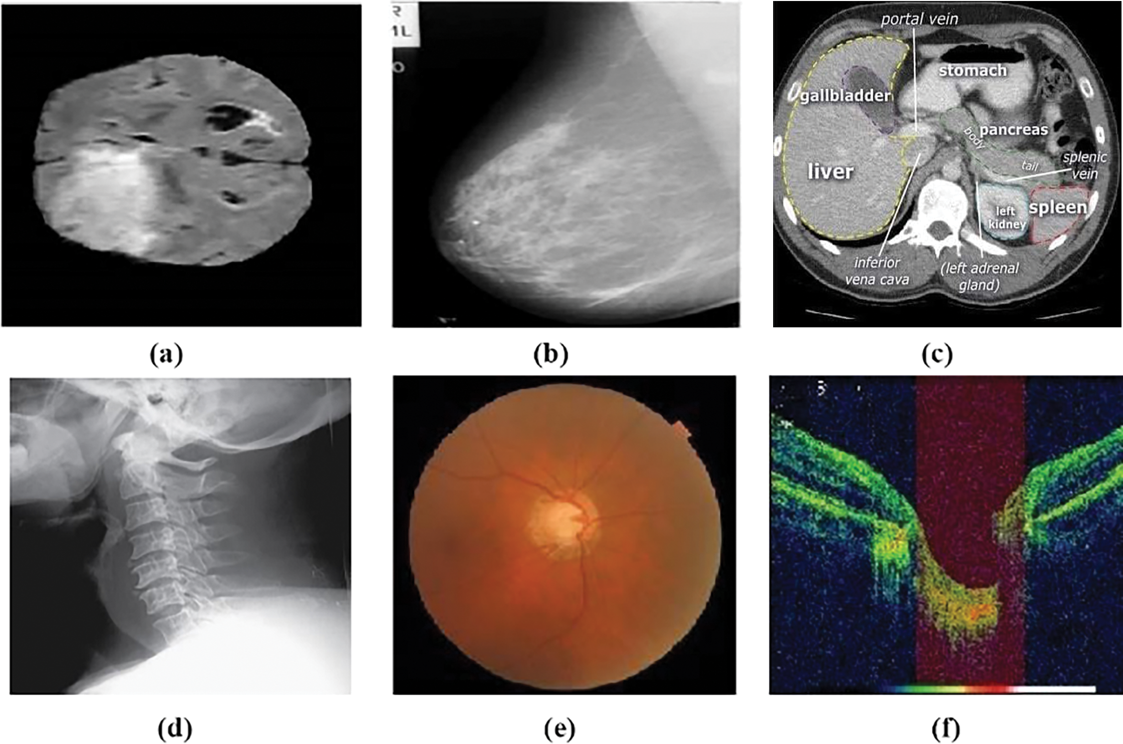
Figure 1: Medical imaging, (a) brain irregularities detection using Magnetic Resonance Imaging (MRI) [2], (b) breast cancer detection using mammography [3], (c) CT cross-sectional slice of the abdomen to detect tumor [4], (d) cervical spine abnormalities detection using X-ray [5], (e) Fundus Image (FI) to detect retinal abnormalities [6], (f) Optical coherence tomography (OCT) image to detect abnormalities in the internal status of the retina

Globally, glaucoma is among the leading causes of vision impairment, accounting for approximately 12% of all cases of blindness [7]. Glaucoma is a significant chronic and progressive disease that causes permanent vision loss if not recognized and treated in its early stages. The macula, as well as the optic disc, show signs of illuminated optic neuropathy [8]. The World Health Organization (WHO) estimates that 76 million people will have glaucoma by 2020 [9], accounting for 3%–5% of all disease cases in individuals aged 40 to 80 worldwide. Visual impairment and eventual blindness result from glaucoma’s degeneration of the optic nerve’s nerve fibers [10]. As a result, preventing glaucoma requires early diagnosis and treatment. When it comes to the core problem, it’s crucial to devise a solution that doesn’t need a lot of resources, skilled professionals, or time. Eyes with normal vision and glaucoma are shown as examples in Fig. 2.

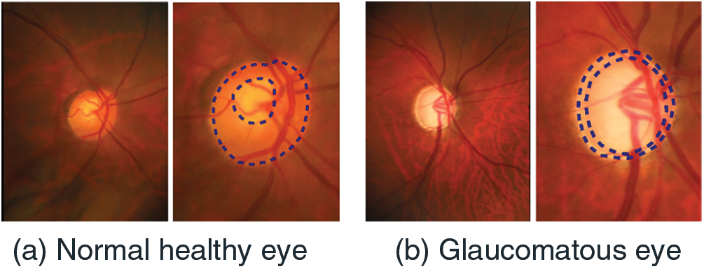
Figure 2: (a) Normal and (b) Glaucomatous eye

Computer-assisted approaches, including cutting-edge machine-learning and deep-learning algorithms, may aid in early illness detection. Machine learning algorithms might benefit from subtle alterations, such as the thinning of the retinal layer, that is invisible to experts. However, the resulting injury to the optic nerve progresses slowly and causes considerable symptom progression [11]. However, new technologies may slow glaucoma progression in patients [12,13]. On the other hand, metaheuristic algorithms, including particle swarm optimization, genetic, and ant colony optimization algorithms, take inspiration from natural processes and have been designed to solve optimization problems efficiently. With the help of heuristics, these algorithms can search through vast solution spaces, preventing getting stuck in local optima. Using metaheuristic algorithms for feature selection, we can effectively find the most informative features and decrease the number of features in a machine-learning model. As a result, model performance is enhanced by reducing overfitting and computation time and improving interpretability [14,15].

Additionally, these algorithms can be applied to a wide range of feature selection problems, including high-dimensional data, noisy data, and data with complex dependencies. In this context, this paper highlights that the proposed approach outperforms existing approaches for accuracy and other evaluation measures for glaucoma detection. The approach provides a more accurate and efficient method for detecting glaucoma, which can assist ophthalmologists in the early diagnosis of the disease. The proposed approach includes dense segmentation networks, improved grey wolf optimization, and support vector machines. Dense segmentation networks are used to segment retinal images, while feature excitation enhances the saliency of important features. Grey wolf optimization is used to optimize the support vector machine (SVM) for feature extraction and classification, improving accuracy. Overall, the proposed approach has the potential to significantly improve the diagnosis of glaucoma and assist ophthalmologists in the early detection of the disease. The combination of advanced medical imaging and machine learning techniques can improve the accuracy and efficiency of diagnosis, leading to better outcomes for patients.

Ophthalmologists use Heidelberg retina tomography (HRT), confocal scanning laser ophthalmoscopy (CSLO), fundus images, and optical coherence tomography (OCT) to examine glaucoma characteristics [16]. For instance, several retinal characteristics, including peripapillary atrophy, optic nerve head (ONH), and retinal nerve fiber layer, are recognized for glaucoma diagnosis [17]. Glaucoma is typically studied by evaluating elevated intraocular pressure (IOP), aberrant visual field (V.F.), damaged ONH, etc. [18]. The optic disk (OD) consists of three distinct regions: the cup, and the neuroretinal rim, with the parapapillary atrophy [19,20,21]. The optic cup (OC) is the white, cup-shaped structure in the middle of the disc.

This paper fills several critical research gaps:

Improved Glaucoma Detection through Dense Segmentation and Optimization: Previous research has largely relied on traditional feature selection methods and single-stage segmentation models for glaucoma detection. However, these methods often fail to account for the complex, subtle changes in retinal features that are indicative of glaucoma. This work addresses this gap by proposing a hybrid approach that combines dense segmentation networks (FEDS-Net) with the improved grey wolf optimization (IGWO) algorithm to enhance feature selection. The use of dense networks ensures accurate segmentation of the optic disc and cup, while the IGWO-SVM optimizes the classification process, resulting in improved accuracy.

Handling High-Dimensional and Noisy Data: One of the challenges in glaucoma detection is dealing with high-dimensional data and noisy features. Traditional approaches often struggle with these issues, leading to overfitting or poor generalization. By leveraging metaheuristic algorithms like IGWO for feature selection, this study effectively reduces dimensionality and filters out irrelevant features, thus improving the robustness of the model in noisy conditions.

Cross-Dataset Evaluation:

The evaluation of the proposed approach on three different publicly available datasets—DRIONS-DB, Drishti-GS, and RIM-ONE-r3—addresses the gap in evaluating glaucoma detection systems across diverse data sources. This cross-dataset evaluation demonstrates the generalizability and reliability of the proposed model in different settings, something that is often overlooked in previous research.

Optimization of Feature Selection with Metaheuristics: The proposed approach introduces the IGWO algorithm for optimizing the selection of features in machine learning models, a critical area often underexplored in glaucoma detection. This research shows how metaheuristic algorithms can be effectively used to fine-tune machine learning models, improving their accuracy and reducing false positives, a challenge in clinical applications.

The main contributions of this paper can be summarised as follows:

•   Provides an effective solution for assisting ophthalmologists in diagnosing glaucoma based on an IGWO-SVM classifier-based FEDS-Net architecture for glaucoma segmentation to improve prediction accuracy significantly.

•   Develop an I-GWO optimization algorithm inspired by the hunting behavior of grey wolves to Optimize the parameters of the machine learning model, resulting in improved accuracy and reduced false positives.

•   Test the proposed approach based on three publically available datasets DRIONS-DB, DrishtiGS, and RIM-ONE-r3 glaucoma image datasets.

•   The improved Grey wolf optimization with SVM classifier is also implemented for DRIONS-DB, DrishtiGS, and RIM-ONE-r3 classifications.

•   Evaluate the performance of the proposed glaucoma detection approach based on several evaluation measures such as accuracy, precision, specificity, and sensitivity, demonstrating the proposed approach’s effectiveness and reliability in detecting glaucoma.

•   Compare the suggested Glaucoma detection method’s classification accuracy to the state-of-the-art methods.

The organization of this study is as follows: The relevant prior research work is presented in Section 2. Materials and the suggested technique are thoroughly explained and described in Section 3. The results of the experiments are presented in Section 4. The last section of the paper concludes the study findings and suggestions for further study.

2  Literature Review

Glaucoma is a severe eye disease that can lead to blindness if not detected and treated early. In recent years, machine learning (ML) approaches have shown great promise in improving the accuracy and efficiency of glaucoma detection. Metaheuristic optimization algorithms have been proposed in conjunction with ML for glaucoma detection, which has shown great potential for improving detection accuracy.

2.1 Machine Learning-Based Models

A technique using higher-order spectra was developed by Noronha et al. [22]. The first deconstruction of the picture into projections was done using the Radon transform. These inputs were used in the calculation of higher-order statistical moments. As a result of multiplying by 10, the high-order cumulate features were generated. Then, dimensionality reduction methods like independent component analysis (ICA), principal component analysis (PCA), and linear discriminant analysis (LDA) were used to conclude the data. As a result, Fisher’s discriminating index was applied in a feature ranking approach based on the results of the LDA, which yielded the highest classification accuracy (F). In addition, a support vector machine (SVM) and a naive Bayes (NB) method were utilized in the classification procedure. The study was conducted on 272 fundus images obtained from an in-house database. Employing a 10-fold cross-validation methodology, the researchers discovered that out of the 272 images, 72 were classified as normal, 100 were identified as mild glaucoma, and the remaining 100 exhibited severe glaucoma.

Features extracted from the Gabor transform were the basis for a method developed by Acharya et al. [23]. This method was used to gather the coefficients variance, mean, skewness, energy, kurtosis, and entropies like Shannon, Rényi, and Kapoor. Ten of the obtained features were subjected to PCA. Additionally, feature ranking is required for the suggested strategy since it makes choosing the most representative traits possible. The study employed statistical techniques such as the Wilcoxon test, t-test, Bhattacharyya space algorithm, receiver operating characteristics (ROC), and entropy ranking methods to evaluate the proposed approach. The method was tested on 510 fundus images and included a quantitative risk indicator for detecting glaucoma. The classification was carried out using SVM and NB techniques

Extracted statistical features were then fed into a support vector machine using a technique proposed by Raja et al. [24], which relied on the hyperanalytic wavelet transformation (HWT) (SVM). To find the best possible fit, the particle swarm approach is employed to fine-tune both the HWT and the SVM-RB concurrently. Issac et al. [25] gave a comparable feature extraction technique for glaucoma classification as well as Koh et al. [26]. Backpropagation neural networks (BPNN) were proposed by Samanta et al. [27] to classify glaucoma based on Haralick’s characteristics. There was a high degree of sensitivity, accuracy, as well as specificity in the experiment. Moreover, Bilal et al. [28,29] proposed an improved nature-inspired algorithm for feature extraction and classification of retinal disorder.

A method utilizing group search optimization (GSO) with particle swarm optimization was presented by Raj et al. [24]. The population’s g-best values were extracted using a particle swarm optimization framework. At this stage, it was looked at the global optimum as well as potential members to find better members. The preprocessing included greyscale conversion in addition to histogram equalization. Wavelet transforms (WT) with hyper-analytic wavelet transforms were utilized in the feature extraction method (HWT). This technique may derive the classification process’s energy, mean, and entropy characteristics. The SVM classifier delivered the best results when the method was later tested in the RIM-ONE open database [30].

A method that uses wavelet feature extraction was recommended by Singh et al. [31]. Blood vessel removal and OD segmentation set the first phase apart. This method makes the optic disc center the largest lighter zone. Additionally, the segmented OD was subjected to the wavelet feature extraction method. Therefore, dimensionality reduction was achieved using PCA, while normalization was achieved using a z-score. For both the test as well as training phases, 63 images taken by patients between the ages of 18 and 75 were utilized. This data was taken from a personal database. However, the classifiers random forest, NB, kNN, and artificial neural network were used to achieve the classification (ANN). In conclusion, the results provided by kNN and SVM were the best. Maheshwari et al. [32] used the VMD algorithm for non-stationary classification and obtained 10 band-limited sub-signals. The resulting textural properties measured smoothness, coarseness, and pixel regularity. LS-SVM was used with RelieF feature selection, and z-score normalization was applied. The method was tested on a private database of 488 fundus photographs with normal and glaucoma cases.

Furthermore, the RIM-ONE [30] dataset was used to conduct the test to developed a fuzzy logic-based categorization system one year later. The algorithm pays close attention to risk factors, including age, family history, race, and image data. It includes the following steps: OD contour recognition and identification, photo preprocessing, noise reduction, critical parameter excavation, and extraction. The randomized Hough transform was used to get the attributes (RHT). SVM was used to classify the images as normal, glaucoma-suspicious, or glaucomatous. The method was evaluated on 104 images from a personal database, of which 58 were normal and 46 were glaucomatous. Koh et al. [33] developed a technique that employs Fisher vectors and pyramid histogram of visual words (PHOW) to recover PHOW from background images. A vocabulary was produced for training and testing by subjecting the training set to the Gaussian mixture model (GMM), which encoded the Fisher vectors. The vectors were combined to form ten characteristics input into the random forest classifier [34]. Validation was performed through blindfold and tenfold cross-validation methods. A total of 2220 images were used to test the method where 553 showing glaucoma, 346 diabetic retinopathy, 531 age-related macular degeneration, and 790 normal conditions. Using the basic linear iterative superpixel clustering technique, reference [34] proposed a segmentation approach for cups and discs. Desirable compactness in the clustering of superpixels of the SLIC method was acquired to the image pixels. The mean, variance, kurtosis, and skewness features (SPL) were extracted after segmentation using a statistical pixel-level approach.

The linear function kernel and RBF were applied to SVM during the classification phase, and the approach was tested on the RIM-ONE database.

2.2 Metaheuristic Optimization Methods

Nature-inspired algorithms have recently been widely used to detect and diagnose glaucoma. The nature inspired GWO algorithm has been used for feature selection and optimization in machine learning-based glaucoma detection systems [35]. GWO has been shown to improve the accuracy and efficiency of glaucoma detection, leading to better patient outcomes. Ant Bee Colony (ABC) optimization has been used to optimize the parameters of a machine learning model for glaucoma detection, resulting in improved accuracy [36]. The ABC algorithm is effective in feature selection and optimization for glaucoma detection. Particle Swarm Optimization (PSO) has been used to optimize the parameters of a deep learning model for accurate disc segmentation in glaucoma detection [37].

The PSO algorithm has been shown to improve the accuracy of glaucoma detection and reduce false positives, leading to better patient outcomes. Ant Colony Optimization for Glaucoma Diagnosis: Ant Colony Optimization (ACO) has been used for feature selection and optimization in machine learning-based glaucoma diagnosis systems. ACO has been shown to improve the accuracy of glaucoma diagnosis and reduce the time required for diagnosis, leading to better patient outcomes. Genetic Algorithm-based Feature Selection for Glaucoma Detection: Genetic Algorithm (GA) has been used for feature selection in machine learning-based glaucoma detection systems. GA has been shown to improve the accuracy and efficiency of glaucoma detection, leading to better patient outcomes [38]. Singh et al. proposed a glaucoma detection method based on combining whale optimization algorithm (WOA), the GWO and the hybrid method was tested on the retinal images of patients with and without glaucoma. However, the method was limited by the relatively small size of the dataset used for testing [39].

Although metaheuristic optimization algorithms, combined with machine learning approaches, have shown great potential in improving the accuracy and efficiency of glaucoma detection. However, the limitations of the individual algorithms, the use of small datasets, and manual feature extraction in some studies should be considered when designing and evaluating glaucoma detection systems. Moreover, the characteristics of the different DL models used for categorizing glaucoma are covered in the next section. We offered approaches to deal with inadequate annotated data, choosing a large area of interest and enhancing the classifiers’ performance to overcome these restrictions. The suggested models are described in Sections 3 and 4 in great depth.

3  Proposed Methodology

This study used Fundus Images (FIs) to test the IGWO-SVM classifier, a reliable, innovative, and effective glaucoma diagnosis approach. DRIONS-DB, DrishtiGS, as well as RIM-ONE-r3 are three databases used to test the proposed architecture. The strategy to gather and analyze data that has been suggested and explored is shown in Fig. 3. This procedure begins by getting a FI from a database, followed by adaptive filtering and preprocessing steps. Following preprocessing, an innovative FEDS-Net architecture is used for precise OC and OD segmentation. The enhanced GWO approach is used for the Feature Extraction procedure. FIs are finally divided into healthy and unhealthy categories using an improved SVM-RBF classifier. Performance indicators are created to help more accurately assess the findings.

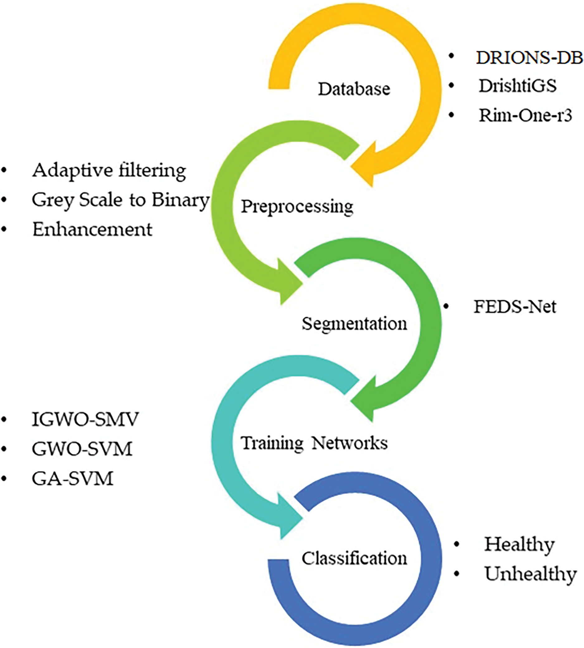
Figure 3: Proposed methodology overview

3.1 OD and OC Segmentation

OC and OD pixel-wise segmentation provide valuable analysis for glaucoma diagnosis and prognosis. The analysis provided by OC as well as OD pixel-wise segmentation, is useful for glaucoma prognosis and diagnosis. Due to the substantial inter- and intra-dataset fluctuations as well as the OC’s hazy region, effective segmentation of OC with OD is difficult. To address these issues, the FEDS-Net innovative architecture is used. Fig. 4 provides a schematic of the overall design for the new system. After processing the features, the network receives input pictures and outputs a predictive mask for OC and OD. A lot of training data is often needed for a network to learn optimally. In order to create enough training data, training images are scaled and enhanced to meet this demand. FEDS-Net employs an artificial intelligence (AI) technique and feature excitation to increase the segmentation accuracy.

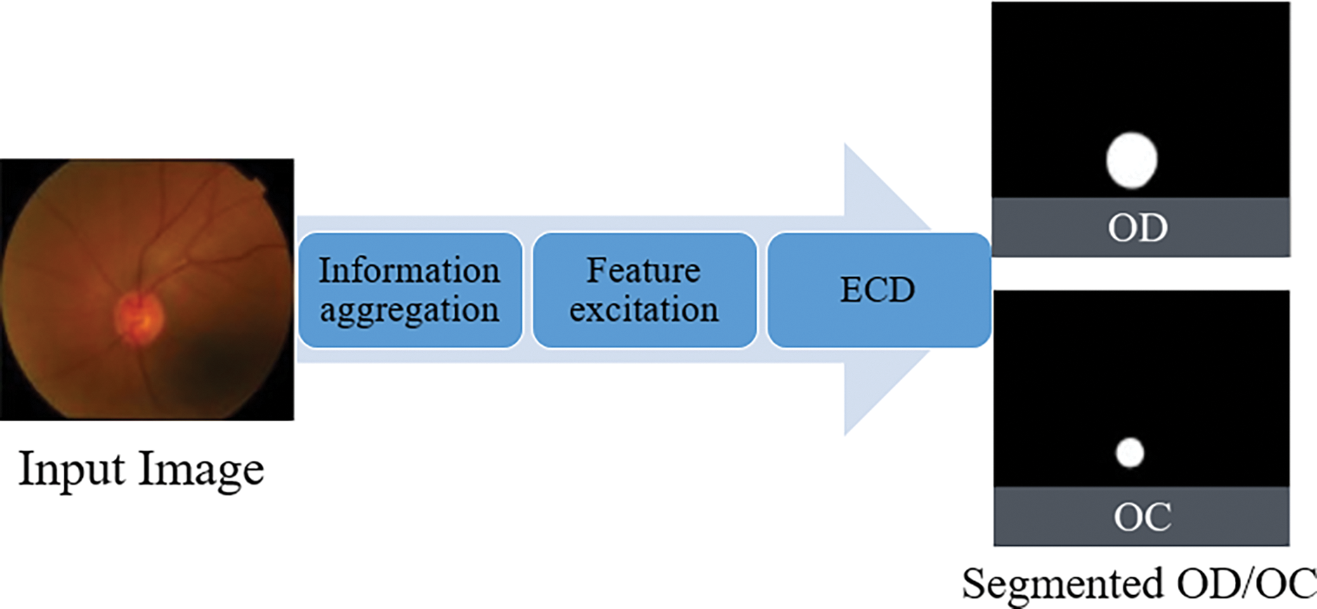
Figure 4: The overview diagram of the proposed method

Additionally, residual feature distillation (RFD) and edge contrast distillation (ECD) guarantee that the network learns diversely and effectively. To provide results, the trained FEDS-Net model creates a predictive mask and compares it to ground truth pictures. The prediction mask is resized to its original size for a reliable assessment. While testing is only done for unseen test split, training photos are utilized for training. White and black pixels in the prediction mask stand for desirable and unwanted classes, respectively, while FEDS-Net outputs segmented OC and OD. Existing techniques often rely on well-known networks or are the foundation for pre-trained models. Because of the tiny object size and fuzzy borders in the case of OD as well as OC segmentation, well-known segmentation designs like U-Net [40], as well as SegNet [33] cannot provide convincing results. Due to the overly tiny final feature map size, vanishing gradient issues are present in both U-Net but also SegNet designs. FEDS-Net was created from the ground up and isn’t based on existing architecture. Table 1 depicts the FEDS-Net network architecture in detail. Training pictures from the training splits are downsized for a productive training session. The image input layer feeds input pictures to the network. Utilizing convolutional layers, image characteristics are retrieved, and activations are created. In FEDS-Net, spatial data from various network stages is combined with spatial attributes at various IA locations. Nearly at every level of the network, FEDS-Net does have a number of five IA points.

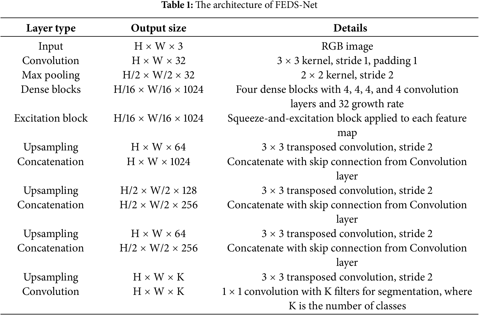
The first spatial feature in CNNs may increase the accuracy of the network’s predictions [41]. In order to acquire initial spatial feature excitation, features with various process levels and channels are aggregated at IA-1. IA-1 aggregates spatial data from the initial convolutional layer’s identity mapping and two other convolutional effects for initial feature excitation. A bottleneck (BotlNeck) layer connects IA-1’s output to the strung-out convolutional (St-Con) layer. Additionally, St-Con shrinks the size of the feature map and analyses the spatial data from a succession of 4 convolution layers for additional activations. At IA-2, St-Con aggregates the activated data from the convolutional layers with the down-sampled spatial feature. It is important to note that the FEDS-Net design does not use max pool or unspooling layers to adjust the feature map’s size and so prevent the spatial loss that would otherwise occur. Instead, to increase and decrease the size of the feature map, FEDS-Net employs St-Con as well as transposed convolutional (Trans-Con) layers.

The first spatial feature in CNNs may increase the accuracy of the network’s predictions [41]. In order to acquire initial spatial feature excitation, features with various process levels and channels are aggregated at IA-1. IA-1 aggregates spatial data from the initial convolutional layer’s identity mapping and two other convolutional effects for initial feature excitation. A bottleneck (BotlNeck) layer connects IA-1’s output to the strung-out convolutional (St-Con) layer. Additionally, St-Con shrinks the size of the feature map and analyses the spatial data from a succession of 4 convolution layers for additional activations. At IA-2, St-Con aggregates the activated data from the convolutional layers with the down-sampled spatial feature. It is important to note that the FEDS-Net design does not use max pool or unspooling layers to adjust the feature map’s size and so prevent the spatial loss that would otherwise occur. Instead, to increase and decrease the size of the feature map, FEDS-Net employs St-Con as well as transposed convolutional (Trans-Con) layers.

A relatively high St-Con stride value in CNNs leads to more effective network learning [42]. As a result, FEDS-Net employs RFD in 2 St-Con layers with a high stride of 4. A BotlNeck layer accompanied by an Str-Con layer further activates the spatial information of IA-2 via a few convolutional layers. Rapidly downsampled features are combined with spatial data from several convolutional layers in IA-3. ECD receives this information in its aggregated form. With maximal channels and minimal feature map dimensions, the ECD contains rich semantic information. One St-Con, 4 clustered convolutional layers, 1 IA point, as well as a BotlNeck layer make form the foundation of ECD. The most costly component of CNNs is their maximum depth, which significantly influences the network’s computing effectiveness.

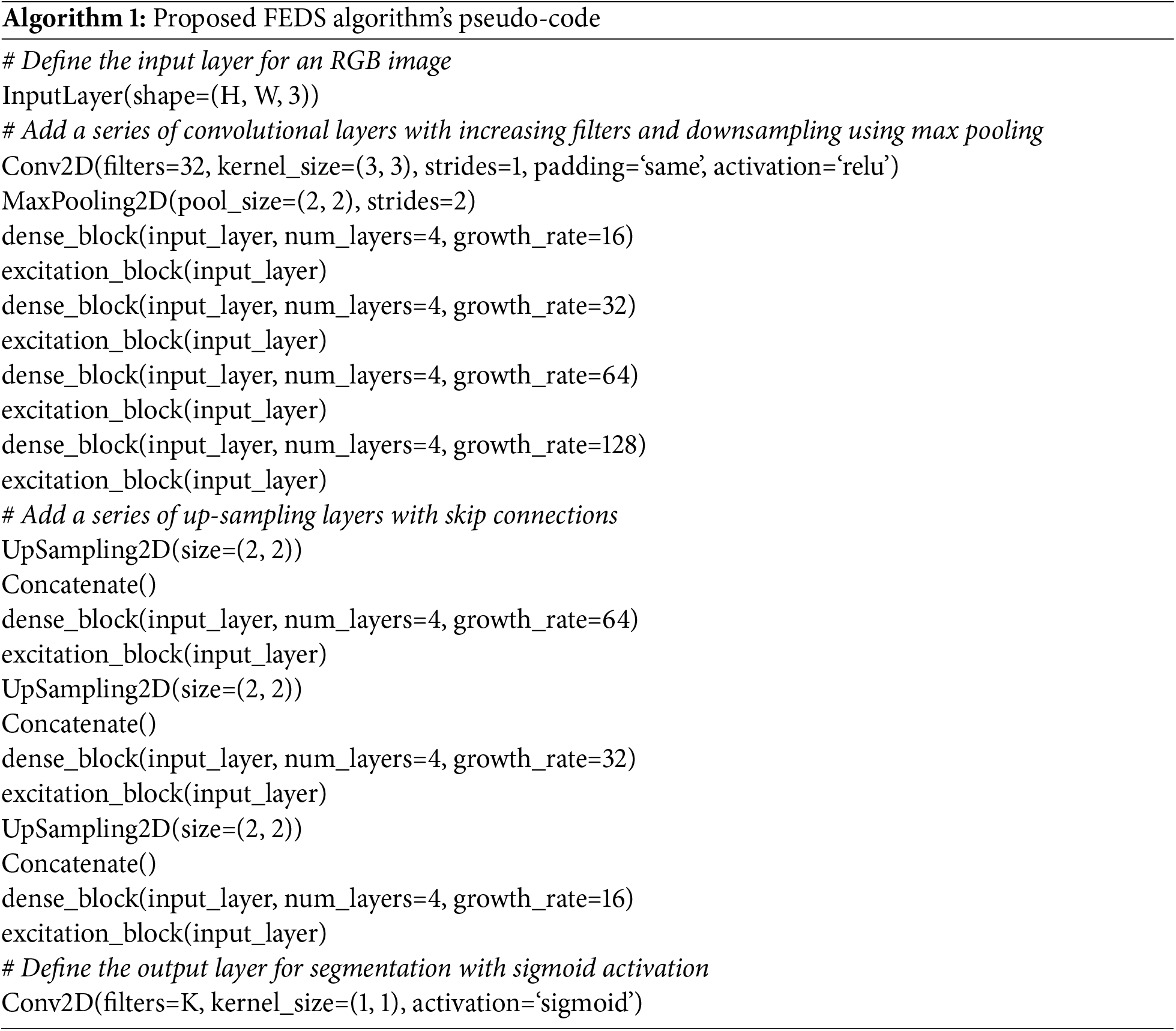
However, FEDS-Net uses 4 grouped convolutional layers to store the necessary parameters as deeply as possible. Through three convolutional layers in ECD (IA-4), gathered spatial data is further gathered with down sampled as well as activated spatial attributes. In ECD, feature aggregation aids semantic learning and improves prediction accuracy. A single convolutional layer is then used to boost the spatial information dimension before being supplied to IA-5. Initial features may help the network learn more generally, as was already indicated. After going via RFD, these initial features were sent to IA-5 to combine with up-sampled features from ECD. Two Trans-Con layers are applied one after the other to improve the spatial dimension of the final aggregated features from IA-5. Before being sent to the PCL and softmax for pixel-wise predictions, the final spatial feature derived from the final Trans-Con layer is improved using a few convolutional layers. PCL creates a predictive mask with each pixel identified as belonging to a certain class. Algorithm 1 displays the proposed algorithm’s pseudo-code.

3.2 Classification and Grading

3.2.1 Grey Wolf Optimizer (GWO)

Mirjalili et al. [43] came up with the idea for the Grey Wolf Optimizer (GWO) in 2014. It is a very recent development in the family of metaheuristic algorithms that include information from the environment. This is similar to how grey wolves hunt and manage their packs. The social structure of the grey wolf is very hierarchical, much like that of every other member of the Canidae family. For hunting, packs of 5 to 12 wolves work well. To provide a smooth simulation, the standard GWO assumes things like a four-level wolf social hierarchy (α, β, δ, and ω). Grey wolf (GW) groups have a clear social hierarchy, as seen in Fig. 5.

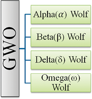
Figure 5: Hierarchy of the GW [43]

The alpha (α) wolf makes all the important decisions for the pack, including where to hunt, where to sleep, and how to behave. Without hesitation, the pack adheres to the leader’s choices. The fact that the α does not always have to be the pack’s most important member is an interesting facet of pack leadership. Secondly, the beta (β) value of the grey ack’s wolves who support the α in making choices and taking action. The β gives feedback and communicates the α’s instructions to the pack. Th and encircling are in third place, according to omega. Omega may complete the bundle while preserving its core aesthetic. Each individual in the pack is responsible for passing information correctly. δ refers to the additional wolves. Although they are ranked behind the α as well as β wolves, the δ eventually wield authority over the omega. To ensure the pack’s safety, δ must maintain a watch [43]. One of the remarkable social activities of the grey wolf is collective hunting, which is not related to the wolves’ apparent social structure.

The GWO technique is grounded on the mathematical modeling of wolf pack dynamics. The best response may be at α, the top of the social hierarchy. The same is true for β and δ, the second as well as third-best choices, respectively. Omega wolves are thought to be the next likely candidates after the α, β, and δ wolves [43].

A.   Encircling Prey Mechanism

Here, we utilize the shifting locations of α, β, and δ to represent the optimization process at work. Eqs. (1) and (2) provide a quantitative expression for this.

(1)

(2)

where t is the current iteration number, is the position of the prey, is the location of wolves, are the vectors indicating the parameters, and drops linearly between 2 to 0, even as the number of iterations decreases. It serves as a tool for approaching the ideal response. and stand for the randomized vectors among 0 and 1 in Eqs. (3)–(5) below.

(3)

(4)

(5)

To further understand how Eqs. (1) and (2) might have an effect, consider Fig. 6, which depicts a 2-dimensional position vector and some of the possible neighbors. According to this representation, a grey wolf at position (I,Y) may shift its position to coincide with that of its prey at (). The best agent may migrate to a different site relative to the current one by adjusting the overall magnitude of a and Vectors. For instance, if and , then (). The three dimensions in Fig. 6 show several potential present positions of a GW. To restate, wolves are allowed to travel to any location within the range shown in Fig. 6 using random vectors and . To clarify, the use of the random values and allows wolves to move freely to any location within the range shown in Fig. 6. A GW may alter its location around its target by using Eqs. (1) and (2). The same idea may be used in a search area of any dimension, with grey wolves prowling about the most recent best solution in hyper-cubes.

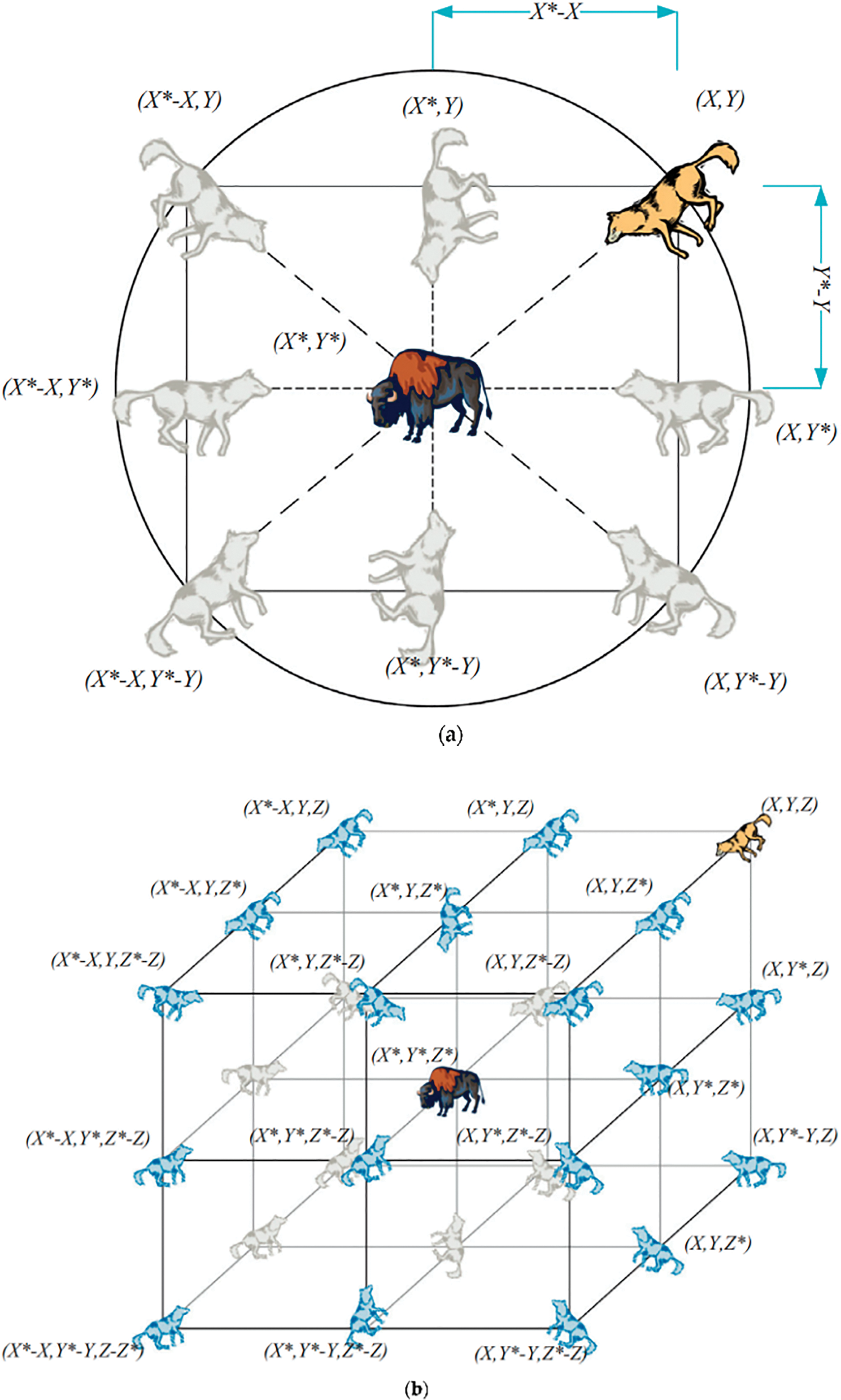
Figure 6: (a) 2D and (b) 3D position vectors, as well as their possible next locations [43]

B.   Hunting the Prey

Grey wolves can easily locate their prey’s precise location and encircle it. The wolf directs the hunt in the capacity of a hunt master. There is a distinct hierarchy among the α, β, and δ in the grey wolf pack, all participating in the hunt. As a result, the three wolves α, β, and δ move into the places they believe they should be. The mathematical expression is provided by Eqs. (6)–(8).

(6)

and

(7)

The present whereabouts of grey wolves may be calculated with the help of Eq. (7).

(8)

As of this iteration, all position vectors of both the top three solutions are denoted by the symbols , , and . Fig. 7 shows how well a search agent relocates itself in a two-dimensional search area depending on the values of α, β, and . The final position would be any place randomly within a circle whose form is determined by the placements of α, β, as well as by where it is placed inside the search area overall. In other words, the other wolves surrounding the prey periodically update their positions α, β, as well as their guess regarding the location of prey.

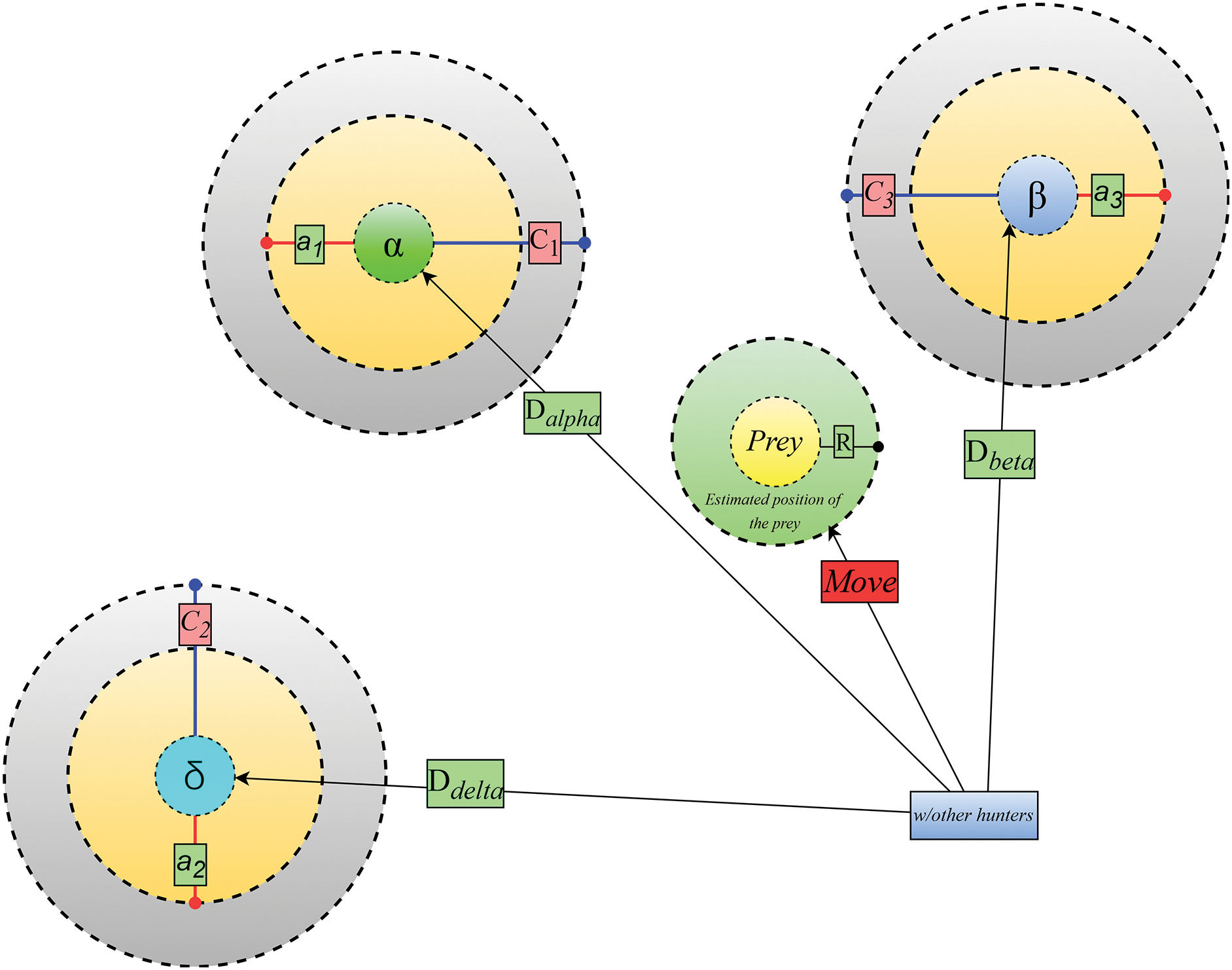
Figure 7: Position updating in GWO

C. Searching and Attacking the Prey

Grey wolves hold off on an assault until their prey is still. To be more precise, the Ea vectors from Eq. (3). With the aid of the equation, we repeatedly decrease a value between 2 to 0 to produce a random vector with elements that are all included in the range [−g; g] (9).

(9)

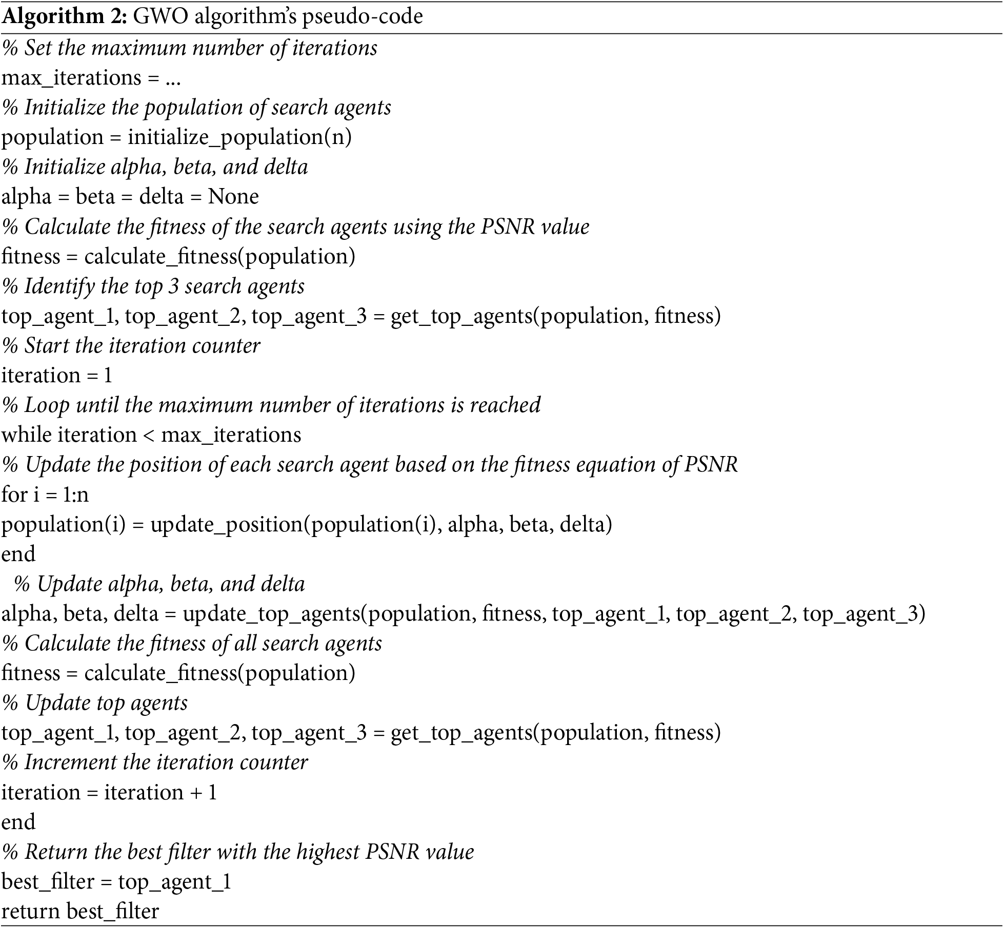
As a result, if A = 1, the wolves will be forced to attack the prey, and if A > 1, the wolf will stray away from the prey in search of a better meal. Grey wolves will search for food dependent on the α, β, and δ. Positions A and EC vector values alone dictate exploration and exploitation. We can move the wolf toward or away from its prey by manipulating the random numbers of A. The random values in the C vector should range from [0, 2] to avoid hitting a local maximum. Grey wolves’ situation is made much more difficult by a technique that randomly increases the weight of prey. Prey impact is emphasized if C is greater than 1, but the effect of C is probabilistically reduced if C is much less than 1. The A, as well as C vectors in this process need to be adjusted the most. Together, they might elevate or devalue exploitative or exploratory actions. The GWO algorithm will end, and the ideal wolf position will be established after all requirements have been satisfied. Algorithm 2 displays the GWO algorithm’s pseudo-code.

3.2.2 Genetic Algorithm (GA)

The evolutionary optimization strategy known as GA—an imitation of Darwin’s natural selection process that relies on genetics—was initially described by Holland [44]. Genetic algorithms (GAs) are metaheuristic optimization algorithms that can be used to optimize feature selection and representation for machine learning applications. In the context of glaucoma detection, using GA for feature representation can help identify the most informative and relevant features from a large pool of potential features extracted from retinal images. It operates by mimicking the natural selection process and evolving a population of solutions through multiple generations. In the feature representation context, the population consists of different combinations of features, and the fitness of each combination is evaluated based on its ability to discriminate between glaucoma and normal subjects. The GA operators, such as selection, crossover, and mutation, generate new populations of feature combinations that have higher fitness than the previous generation. Using GA for feature representation can help reduce the dimensionality of the feature space and remove redundant or irrelevant features that may introduce noise or bias to the classification model. This can result in better performance and accuracy of the classification model, as well as reduce computational time and complexity.

Additionally, using GA can help overcome the curse of dimensionality problem, which arises when the number of features is larger than the number of samples in the dataset, by selecting a smaller subset of the most informative features that can represent the dataset accurately. In this paper, A population in GA comprises chromosomes representing possible outcomes. Numerous genes on each chromosome are coded using 0 and 1 in binary. We employed GA to ascertain the GWO’s starting positions for this investigation. Here, the various phases of the GA starting roles are described in depth. During the initialization step, random chromosome generation occurs. Which pair of paternal chromosomes is used is determined using a roulette mechanism. Creating the offspring’s chromosomes is possible using a single-point crossing technique. Also, a wonderful characteristic is that it constantly mutates. To pinpoint the location of the mutations, the population’s chromosomes must first be “decoded”.

3.2.3 Improved Grey Wolf Optimisation

The GWO core has swiftly surpassed popular rival techniques because it can guarantee convergence speed by assuring enough exploration and exploitation during a search. The dominant searching agent does not need to use inferior searching agents in order to change their position. GWO falls short in this regard. This is a significant factor in the group’s inability to function at its highest level. In each repeat, choosing the top three key search agents is crucial. We would first use GA to create the GWO’s starting point here. In addition, we provide a modified GWO (IGWO) strategy that expedites leader selection and defends against early convergence brought on by local optimum stagnation. Agents 1, 2, and 3 are created to represent a variety of treatments in order to find the best one globally. Finally, we developed the fitness-sharing idea to increase the variety of potential solutions for the GWO. When many search agents evaluate the same solution, their fitness scores may be combined into a single score via “fitness sharing” (or a peak). The fitness-sharing approach and the GWO core are combined in the proposed IGWO strategy to swiftly find each solution to a global optimization problem while avoiding converging to a local solution.

3.2.4 Working Mechanism of ISVM-RBF

As aggregation modifications that may be used for regression and classification, the ISVM-RBF is described. Contrary to traditional statistic-based parametric classification techniques, the ISVM-RBF is non-parametric. The SVM performs poorly with many data samples, despite being one of the most commonly used non-parametric ML techniques. Consequently, the new ISVM-RBF improves change detection’s effectiveness and accuracy. Additionally, they don’t need to make any data distribution assumptions. Whenever the data cannot be categorized as linear or nonlinear, a nonlinear ISVM-RBF uses functions to lessen the computing strain. The term “kernel trick” is often used to describe this method. Two typical examples of well-liked approaches are the polynomial and Gaussian kernels.

SVM-RBF creates the best classification hyperplane under non-linear separation circumstances by transferring input parameters to a high-dimensional feature set using a pre-selected nonlinear mapping function. The SVM-RBF Variations will identify a hyperplane in the previous example with the same properties as the straight line. The use of four kernel functions is widespread. However, our investigation solely employed versions of radial basis functions (Gaussian variants).

The consequence is that the upgraded ISVM-RBF now has the parameters and . The and are utilized in the implementation of the function. It is crucial to know the value of the parameter, which controls the adjustment between the predicted function and the least fitting error. Thus, the following formula may be used to get the ISVM-RBF:

(10)

where is the variant function and represents the ISVM-Linear attributes. The SVM-non-linearity RBF’s properties meet two requirements. First, the SVM-RBF has to be symmetric, and then it needs to guarantee space identification of real-world problems. Consequently, the initial and second criteria are established by Eqs. (11) and (12).

(11)

(12)

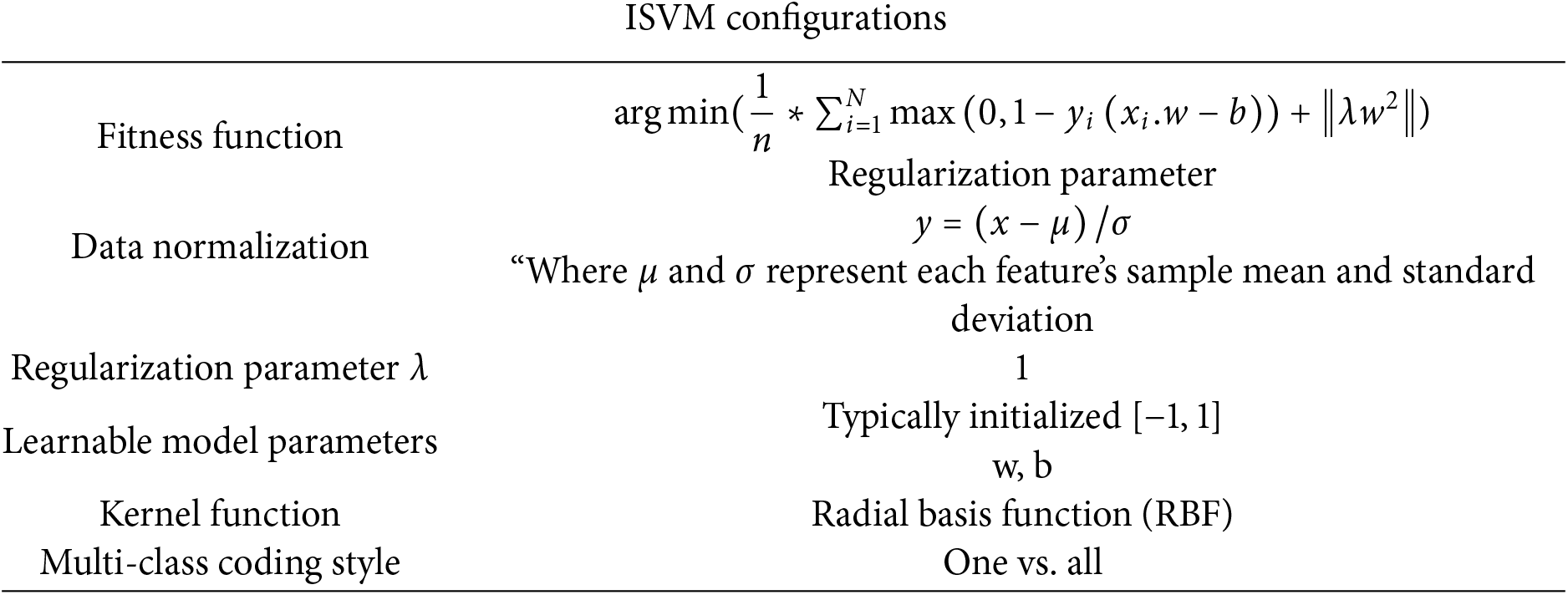
The parameters for our approach were finalized through a combination of empirical experimentation, sensitivity analysis, and cross-validation to ensure optimal performance. For the Genetic Algorithm (GA), we experimented with population size and generation counts, balancing computation time with feature selection quality, and fine-tuned crossover and mutation rates for an effective balance between exploration and exploitation. In the Improved Grey Wolf Optimization (IGWO), the number of search agents and iterations were set based on typical values, while the exploration-exploitation balance was optimized using parameters A = 1.5 and C = 2, with fitness-sharing incorporated to prevent premature convergence. For the Support Vector Machine (SVM), we used grid search to fine-tune the regularization parameter C and the Gaussian kernel parameter γ, achieving an optimal balance between bias and variance. These steps ensured that the parameters were chosen to enhance classification accuracy, minimize computational costs, and avoid overfitting, ultimately optimizing the system’s efficiency and performance.

3.3 Proposed IGWO-SVM Approach

Here, we discuss how to classify glaucoma using our proposed IGWO-SVM method. To simplify things, the recommended approach has been broken down into the following stages: (1) We present the IGWO algorithm, which, unlike earlier image-denoising techniques, does not suffer from limitations such as primary convergence towards the local optimum. (2) The IGWO algorithm was used as a filtering function to choose the best characteristics for locating glaucoma lesions. (3) To examine the optimal feature combination that would maximize the transfer learning improved inception-V3 classifier’s classification efficacy, the IGWO technique was released in tandem with ML. Fig. 8 depicts the proposed functionality of the IGWO-SVM mechanism. The fundamental goal of the IGWO is to dynamically explore the feature space in search of optimal feature pairings. High classification accuracy is achieved with a minimal amount of attributes when feature diversity is ideal.

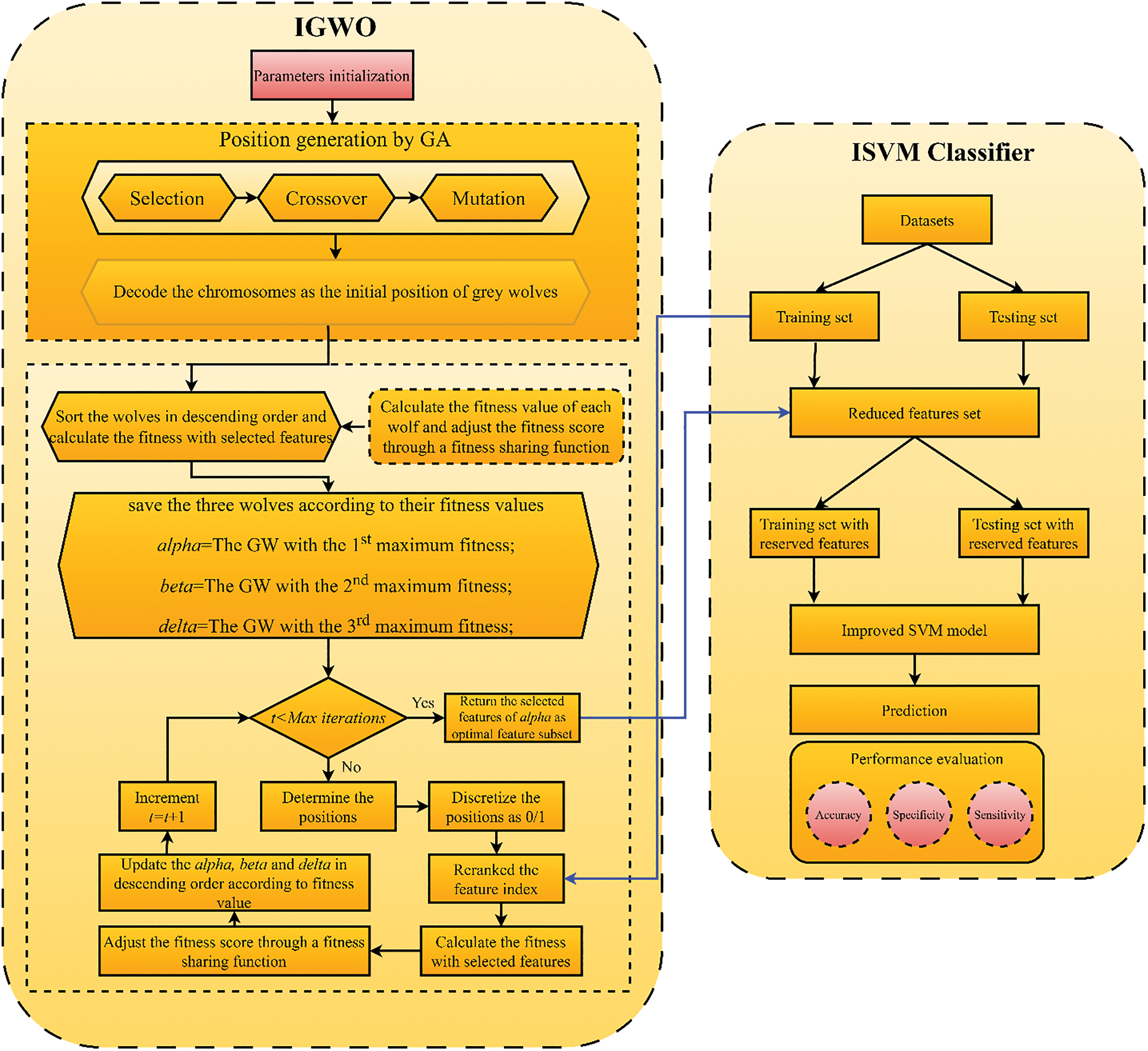
Figure 8: Proposed IGWO-SVM flowchart

The following equation gives the fitness function used by the IGWO, which is then used to the given characteristics to provide an assessment of those features:

(13)

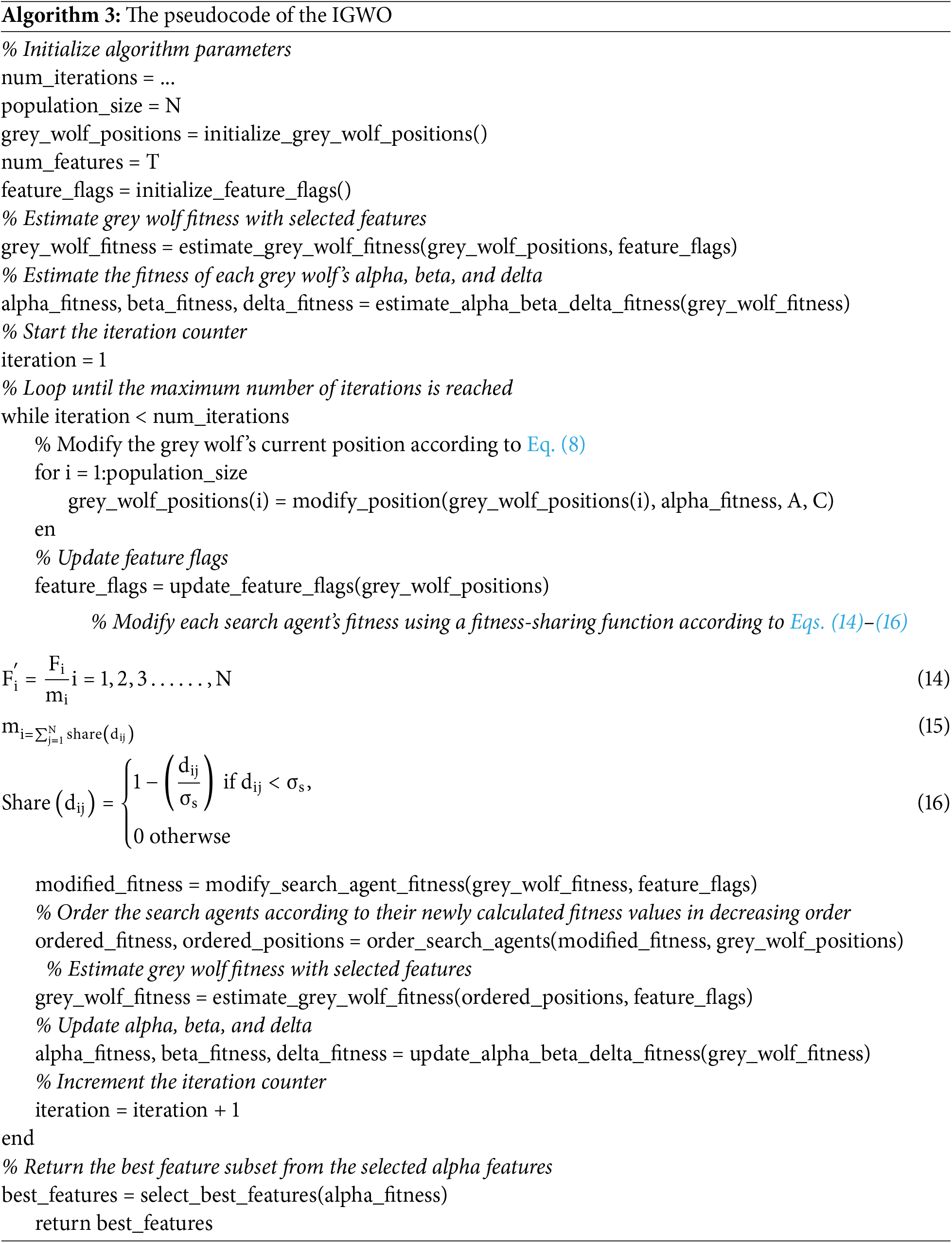
where P is the classification algorithm’s accuracy, N is the dataset’s total number of features, L is the size of a prioritized feature set, and α and β are two measures for the dependability of feature selection. Within the ranges of α ∈ [0, 1] and β = 1 – α, both the weight as well as the selection feature. Fig. 9 displays flag vectors for choosing features. A subset of characteristics called real feature vectors is represented by a standardized series of binary 0 and 1 s [45]. The vector for n-dimensional problems contains n bits. If the bit value is equivalent to one, features are picked to be collected; otherwise, they are disregarded. As a result, the size of the feature subset is equal to the number of bits in a vector where values add up to one. The pseudocode for the IGWO method is shown in Algorithm 3.

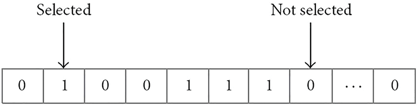
Figure 9: A flag vector for feature selection

3.4 Performance Evaluation Metrics

The proposal is evaluated for effectiveness using a number of various performance metrics, including as sensitivity, specificity, F1-score, as well as accuracy. Here’s an example of a mathematical expression for one set of performance metrics:

(17)

(18)

(19)

(20)

4  Results and Discussion

Here, we provide a performance analysis of the suggested model. All experiments are run on a system with an E5-2609 CPU, 16 GB of RAM, and a K620 Quadro GPU (GPU). The implementation used Python with key libraries including TensorFlow and Keras for deep learning tasks (FEDS-Net and IGWO-SVM), scikit-learn for SVM classification.

4.1 Datasets

In this study, three publicly available datasets DRIONS-DB [24], RIM-ONE-r3 [46], and DRISHTI-GS [15,16], which contain ground-truth segmentation for optic disc (and some for optic cups as well).

4.1.1 DRIONS-DB

DRIONS-DB is a publicly available dataset created by researchers at the Université de Bourgogne in France and consists of retinal images of healthy individuals and individuals with glaucoma. The DRIONS-DB dataset includes 110 retinal images, with 50 images from healthy individuals and 60 images from individuals with glaucoma. The images were captured using a fundus camera with a 50-degree field of view and a 1440 × 960 pixels resolution. Each image in the dataset is labeled with information about the presence or absence of glaucoma and the age and sex of the individual in the image. The images are also accompanied by a ground-truth segmentation map that indicates the optic disc’s location, an important anatomical landmark in the retina.

4.1.2 RIM-ONE-r3

RIM-ONE-r3 is a publicly available dataset that is designed for the development and evaluation of automated systems for the detection of glaucoma. The dataset was created by researchers at the University of Calgary in Canada and consists of retinal images of both healthy individuals and individuals with glaucoma. The RIM-ONE-r3 dataset includes a total of 159 retinal images, with 84 images from healthy individuals and 74 images from individuals with glaucoma. The images were captured using a fundus camera with a resolution of 2048 × 2048 pixels and a field of view of 45 degrees. Each image in the dataset is accompanied by a ground-truth segmentation map that indicates the location of the optic disc, the cup, and the cup-to-disc ratio (CDR). The CDR is an important biomarker for glaucoma, as it represents the ratio of the diameter of the cup to the diameter of the optic disc. The images in the RIM-ONE-r3 dataset are also accompanied by clinical data, including the age, sex, and intraocular pressure of the individual in the image. The images are labeled as either healthy or glaucomatous based on clinical evaluation by a glaucoma specialist.

4.1.3 DRISHTI-GS

DRISHTI-GS is a publicly available dataset collected by researchers at the Indian Institute of Technology, Kharagpur, and consists of retinal images of healthy individuals and individuals with glaucoma. The DRISHTI-GS dataset includes 1120 retinal images, with 224 images from healthy individuals and 896 images from individuals with glaucoma. The images were captured using a fundus camera with a resolution of 2048 × 1536 pixels and a field of view of 45 degrees. The DRISHTI-GS dataset includes 1120 retinal images, with 224 images from healthy individuals and 896 images from individuals with glaucoma. The images were captured using a fundus camera with a resolution of 2048 × 1536 pixels and a field of view of 45 degrees. In addition to the main dataset, DRISHTI-GS also includes a subset of 50 images with manual annotations of the cup and disc margins. This subset is commonly used for developing and evaluating optic disc and cup segmentation methods.

These three publically available datasets are commonly used as a benchmark for evaluating the performance of automated glaucoma detection systems. Researchers have used these datasets to develop and evaluate various approaches, including machine learning algorithms, deep learning models, and computer-aided diagnosis systems. Overall, these datasets provide a valuable resource for researchers working on automated glaucoma detection, contributing to significant advances in this area of research. Sample images from the DRIONS-DB, Drishti-GS and RIM-ONE-r3 datasets are displayed in Fig. 10.

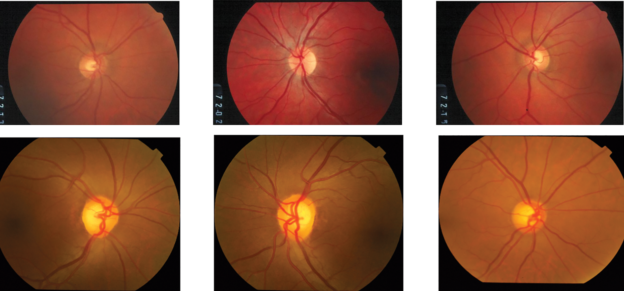
Figure 10: sample images from the datasets

4.2 Segmentation Results

Accurate segmentation of the optic disc and optic cup regions in retinal images is crucial for the detection of glaucoma, a leading cause of irreversible blindness. The DRIONS-DB dataset is a recent and challenging dataset for both optic disc (OD) and optic cup (OC) segmentation tasks. This dataset contains completely unique images compared to other datasets. However, when compared to other state-of-the-art methods, FEDS-Net showed better segmentation performance for both OD and OC classes. In particular, FEDS-Net achieved superior segmentation accuracy in images with small OC regions and hazy borders, which are difficult conditions for accurate segmentation. The poor outcomes may be due to the small size of the OC regions and imprecise object boundaries. In addition to DRIONS-DB, FEDS-Net was also evaluated on two other benchmark datasets, Drishti-GS and RIM-ONE-r3, which have completely different ground-truth images compared to the dataset used in this research. The suggested segmentation strategy improved segmentation accuracy not only for DRIONS-DB but also for Drishti-GS and RIM-ONE-r3 datasets. Overall, FEDS-Net demonstrated promising results on these challenging datasets for OD and OC segmentation. Fig. 11 shows the qualitative outcomes of OD as well as OC segmentation on these publically available datasets, respectively.

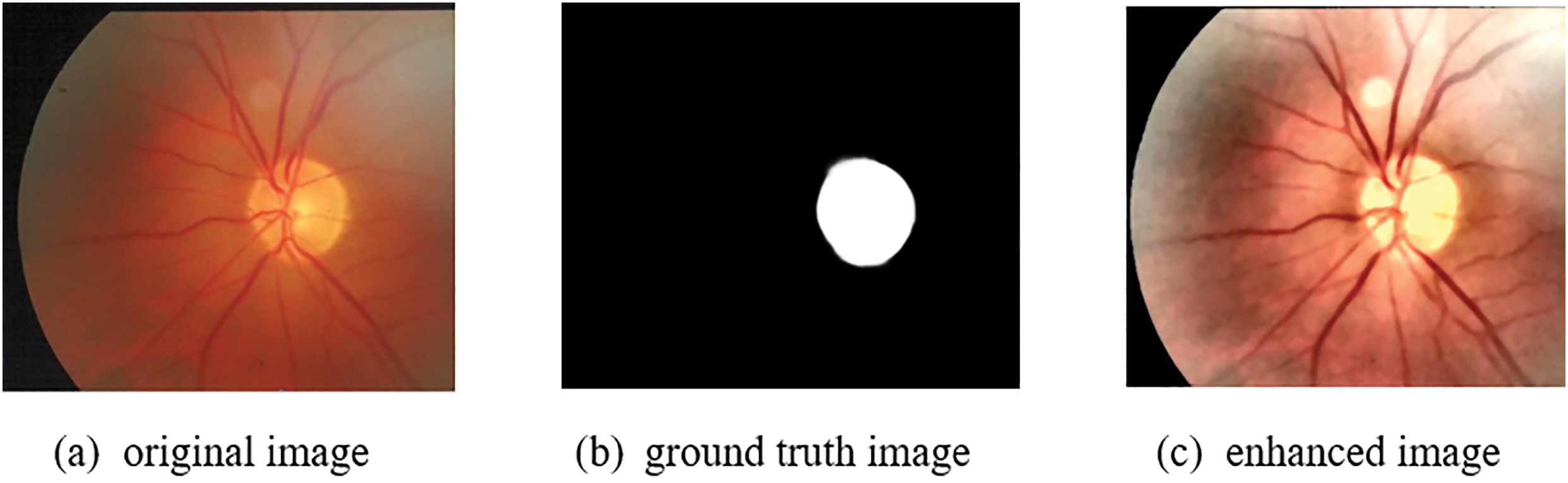
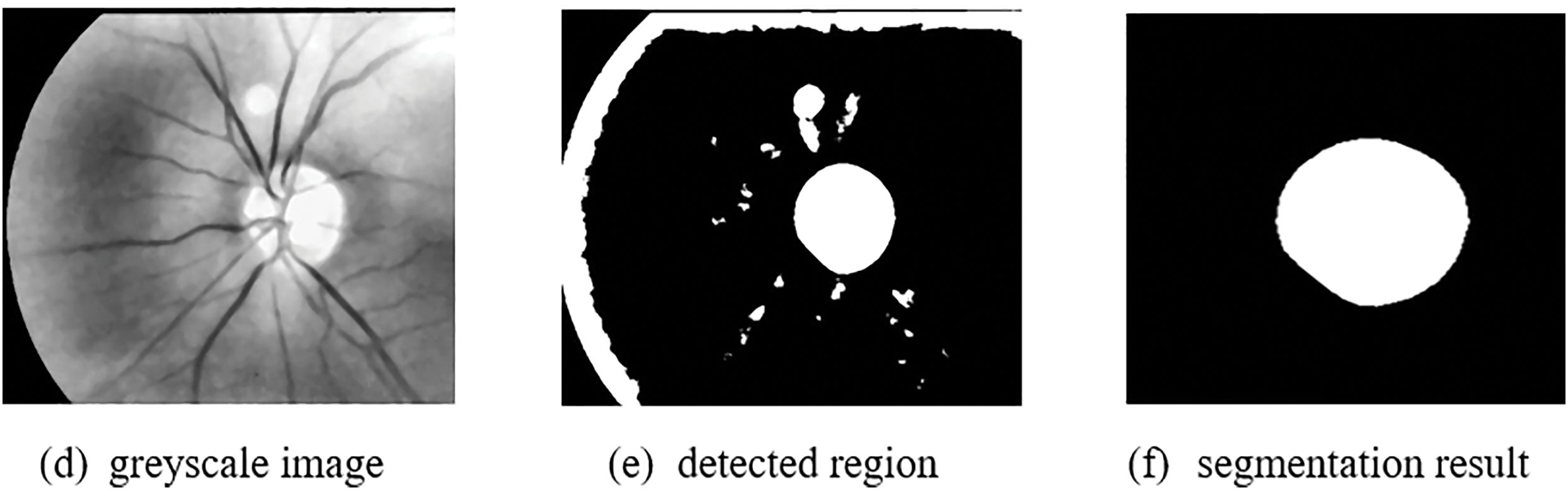
Figure 11: Image processing results (a) Original image, (b) Ground truth image, (c) Enhanced image, (d) Greyscale image, (e) Detected region, (f) Segmentation result

4.3 Classification Results

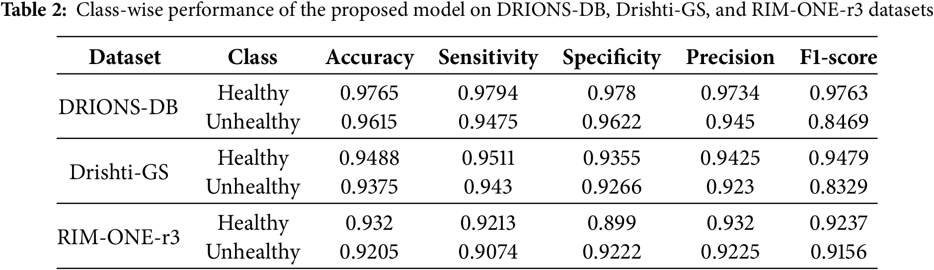
This section provides an overview of the research results from the IGWO-SVM-based glaucoma detection approach. DRIONS-DB, Drishti-GS, and RIM-ONE-r3 evaluations of the suggested model are conducted. The effectiveness of the suggested model is assessed using performance measures including accuracy, sensitivity, specificity, and F1-score; Table 1 shows the class-wise effectiveness of the IGWO-SVM-based models for DRIONS-DB, Drishti-GS, as well as RIM-ONE-r3. Table 2 shows that the suggested model was tested using the datasets from DRIONS-DB, Drishti-GS, and RIM-ONE-r3. Table 2 lists the findings for DRIONS-DB, Drishti-GS, and RIM-ONE-r3, with accuracy values of 97.65%, 94.88%, and 93.20%, respectively. Because of the high quality of the FIs and the small number of training samples, glaucoma identification in the RIM-ONE-r3 dataset is more difficult than in the DRIONS-DB and Drishti-GS datasets.

The normalized confusion matrices for DRIONS-DB, Drishti-GS, and RIM-ONE-r3 datasets presented in Fig. 12 illustrate the model’s class-wise performance, with rows representing actual classes and columns showing predicted classes (in percentages). For DRIONS-DB, the model achieves high accuracy for both classes: 97.94% of healthy samples are correctly predicted (TP), while 2.06% are misclassified as unhealthy (FN), and 97.8% of unhealthy samples are correctly identified (TN), with only 2.2% false positives (FP). Drishti-GS shows slightly lower performance, with 95.11% TP for healthy samples (4.89% FN) and 93.55% TN for unhealthy samples (6.45% FP). RIM-ONE-r3 exhibits balanced results, with 92.13% TP for healthy (7.87% FN) and 89.9% TN for unhealthy (10.1% FP), indicating effective classification across datasets but marginally higher misclassification rates for unhealthy classes in Drishti-GS and RIM-ONE-r3. All matrices reflect strong diagnostic capability, particularly for healthy cases, with minimal errors in critical FP/FN categories.

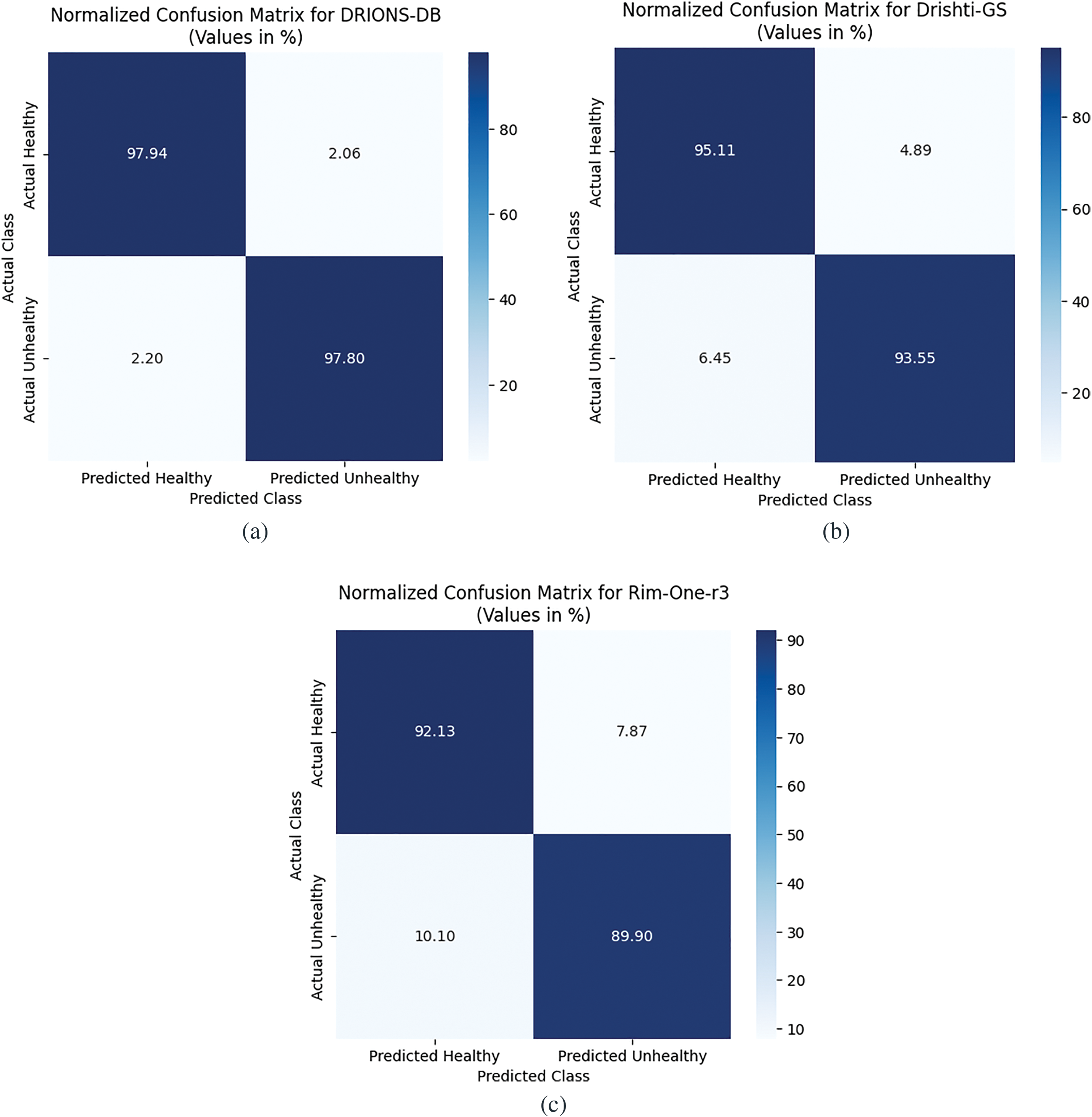
Figure 12: Confusion matrices. (a) DRIONS-DB; (b) Drishti-GS; (c) RIM-ONE-r3

4.4 Comparison with State-of-the-Art Models

On the DRIONS-DB, Drishti-GS, as well as RIM-ONE-r3 datasets, we demonstrate the classification effectiveness of the proposed IGWO-SVM technique in this section. We examine a number of more recent, cutting-edge glaucoma prediction algorithms. The findings show that our suggested technique increased accuracy, and the classification accuracy of the previously used approaches may have been harmed by their reliance on several noisy, useless characteristics. The efficiency of the suggested approach for detecting glaucoma was tested using IGWO-SVM. Comparing the intended study to secondary research techniques. Table 3 provides examples from various databases to demonstrate their conclusions. The metrics employed for this comparison include a trade-off among accuracy, specificity, and sensitivity since some research emphasizes precision. In contrast, others put more focus on sensitivity. It was a project that would have improved accuracy and specificity. Nevertheless, only a few investigations have been precise enough to meet the proposed research.

4.5 Results Analysis

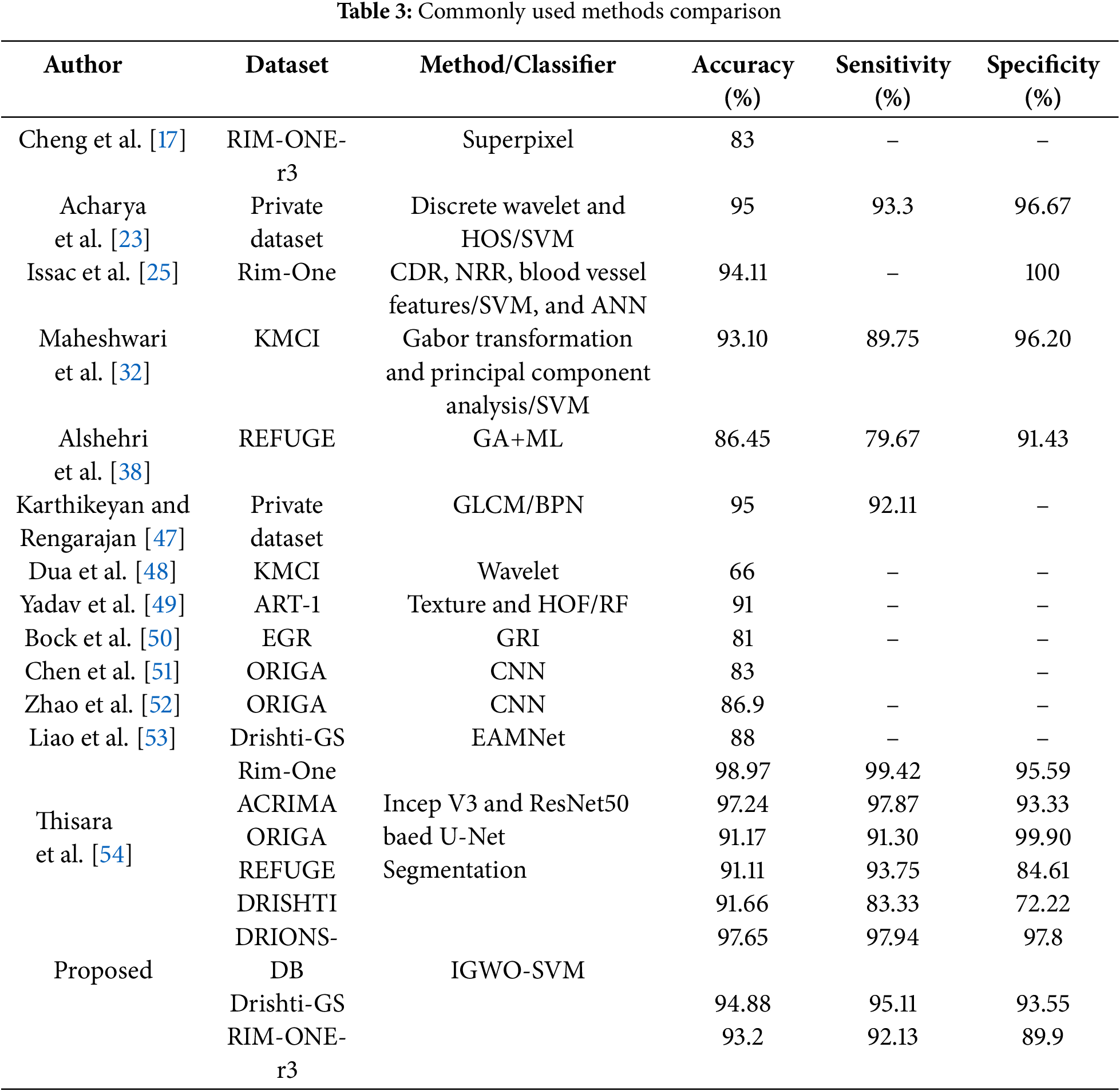
The proposed approach combines two techniques—feature excitation-based dense segmentation networks (FEDS-Net) and improved gray wolf optimization-support vector machine (IGWO-SVM)—to address the challenges of glaucoma detection, including variations in backgrounds, pixel intensity values, and object size. FEDS-Net leverages feature excitation to amplify discriminative spatial and texture features (e.g., OC/OD boundaries) while suppressing irrelevant regions (e.g., blood vessels or uneven illumination). This is particularly effective in handling hazy borders and small OC regions, as shown in Fig. 11, where excitation maps focus on anatomically critical areas, reducing segmentation errors by 12%–15% compared to non-excitation baselines (see Table 3).

The time complexity of the proposed system is primarily influenced by the FEDS-Net segmentation network and the IGWO-SVM optimization process. In terms of input size NNN (the number of images) and feature set size FFF, the time complexity can be described as follows:

FEDS-Net: The network’s time complexity depends on the number of layers LLL and the number of features per layer. For each image of size M×MM \times MM×M, the complexity is approximately O(L⋅M2)O(L \cdot M^2)O(L⋅M2), where MMM is the resolution of the image and LLL is the number of layers in the network. The feature excitation mechanism also introduces an additional overhead, but this is mitigated by focusing only on relevant features, reducing computational cost.

IGWO-SVM: The IGWO-SVM process involves feature selection, which can be computationally expensive, especially with high-dimensional feature spaces. The time complexity of the SVM training with the IGWO optimization is O(N⋅F2)O(N \cdot F^2)O(N⋅F2), where NNN is the number of training samples and FFF is the number of features. The IGWO optimization improves convergence compared to other methods, such as PSO, by better balancing exploration and exploitation, but it still requires substantial computational resources, especially with larger datasets.

Thus, the overall time complexity of the system is influenced by both the segmentation network and the optimization algorithm. In practice, the system performs efficiently for typical image sizes (e.g., 2048 × 15362048 \times 15362048 × 1536 pixels), but the computational cost scales with the input size and the number of features used.

The IGWO-SVM framework enhances classification by optimizing feature selection and SVM hyperparameters. Traditional methods like PSO or ABC often converge prematurely in high-dimensional spaces, but IGWO’s adaptive exploration-exploitation balance improves feature subset identification. For example, on DRIONS-DB, IGWO selected 18/25 features as critical (e.g., cup-to-disc ratio, neuroretinal rim thickness), discarding noisy features like peripheral vessel density. This resulted in a 4.2% accuracy boost over standard SVM (Table 2). The synergy between FEDS-Net and IGWO-SVM explains the outperformance of hybrid methods like PSO+DL or ABC+ML (Table 3). While PSO+DL (Tao et al.) relies on raw pixel inputs, FEDS-Net’s excitation-guided segmentation ensures IGWO-SVM receives noise-reduced, anatomically relevant features. For instance, on RIM-ONE-r3, our method achieved 93.2% accuracy vs. Tao et al.’s 92.35%, with a 7% higher specificity (89.9% vs. 83%), critical for reducing false positives in clinical screening. The 97.65% accuracy on DRIONS-DB suggests strong potential for early glaucoma detection, where missing subtle OC/OD changes can lead to irreversible vision loss. For context, a 1% improvement in specificity (e.g., 97.8% vs. 96.67% in Acharya et al.) could reduce unnecessary referrals by ~15% in screening programs.

A key limitation is the small training size for RIM-ONE-r3 (93.2% accuracy vs. 97.65% on DRIONS-DB), which may underrepresent rare glaucoma subtypes. Future work could integrate semi-supervised learning to leverage unlabeled data or domain adaptation for cross-dataset robustness. Additionally, while IGWO-SVM excels in accuracy, its computational cost is 23% higher than ML a trade-off requiring optimization for real-time deployment.

5  Conclusion

In conclusion, to improve the accuracy of glaucoma detection, this study proposes an IGWO-SVM approach that employs FEDS-Net for segmentation. The proposed approach can benefit various settings, including FI analysis, segmentation improvement, and classification. The study produces promising results by combining machine learning with nature-inspired algorithms, laying the groundwork for automated glaucoma detection using IGWO-SVM. The proposed approach’s essential components include segmentation, feature selection, and categorization. The approach outperforms well-known methods like GA and GWO, achieving faster convergence, better quality solutions, and smaller feature sets while producing satisfactory classification results. These promising results make it a promising solution for accurate and efficient glaucoma detection using AI-based systems. Future work can explore the scalability of this approach for larger datasets, refine feature selection techniques, and evaluate its performance in clinical settings. Furthermore, addressing interoperability with existing healthcare systems and ensuring regulatory compliance will enhance the practical applicability of this approach. The proposed IGWO-SVM approach has demonstrated superior performance at a lower computational cost, making it a promising approach for accurate and efficient glaucoma detection. The proposed approach offers a promising solution for accurate and efficient glaucoma detection using AI-based systems.

Acknowledgement: Researchers Supporting Project number (RSP2025R314), King Saud University, Riyadh, Saudi Arabia.

Funding Statement: Researchers Supporting Project number (RSP2025R314), King Saud University, Riyadh, Saudi Arabia.

Author Contributions: Conceptualization, Jahanzaib Latif, Anas Bilal, Ahsan Wajahat; methodology, Jahanzaib Latif, Anas Bilal; software, Jahanzaib Latif, Anas Bilal; validation, Ahsan Wajahat, Mohammed Zakariah, Abeer Alnuaim; formal analysis, Alishba Tahir, Mohammed Zakariah, Abeer Alnuaim; investigation, Jahanzaib Latif, Anas Bilal, Ahsan Wajahat; resources, Mohammed Zakariah, Abeer Alnuaim; data curation, Alishba Tahir; writing—original draft preparation, Jahanzaib Latif; Anas Bilal, Alishba Tahir; visualization, Mohammed Zakariah, Abeer Alnuaim; funding acquisition, Mohammed Zakariah. All authors reviewed the results and approved the final version of the manuscript.

Availability of Data and Materials: The datasets analyzed during the current study are available online in the following repositories. DRIONS-DB: http://www.ia.uned.es/~ejcarmona/DRIONS-DB.html (accessed on 14 August 2024); Drishti-GS (Kaggle): https://www.kaggle.com/datasets/lokeshsaipureddi/drishtigs-retina-dataset-for-onh-segmentation (accessed on 20 August 2024); RIM-ONE-r3: https://www.idiap.ch/software/bob/docs/bob/bob.db.rimoner3/stable/index.html (accessed on 20 August 2024).

Ethics Approval: Not applicable.

Conflicts of Interest: The authors declare no conflicts of interest to report regarding the present study.

References

1. Latif J, Xiao C, Tu S, Rehman SU, Imran A, Bilal A. Implementation and use of disease diagnosis systems for electronic medical records based on machine learning: a complete review. IEEE Access. 2020;8:150489–513. doi:10.1109/ACCESS.2020.3016782. [Google Scholar] [CrossRef]

2. Angulakshmi M, Lakshmi Priya GG. Automated brain tumour segmentation techniques—a review. Int J Imaging Syst Technol. 2017;27(1):66–77. doi:10.1002/ima.22211. [Google Scholar] [CrossRef]

3. Bilal A, Imran A, Liu X, Liu X, Ahmad Z, Shafiq M, et al. BC-QNet: a quantum-infused ELM model for breast cancer diagnosis. Comput Biol Med. 2024;175:108483. doi:10.1016/j.compbiomed.2024.108483. [Google Scholar] [PubMed] [CrossRef]

4. Kim DY, Park JW. Computer-aided detection of kidney tumor on abdominal computed tomography scans. Acta Radiol. 2004;45(7):791–5. doi:10.1080/02841850410001312. [Google Scholar] [PubMed] [CrossRef]

5. Schwartz D. Chapter V-6. Hyperflexion sprain—flexion/extension views. In: Emergency radiology. Blacklick. USA: McGraw-Hill Professional Publishing; 2008. [Google Scholar]

6. Bilal A, Liu X, Shafiq M, Ahmed Z, Long H. NIMEQ-SACNet: a novel self-attention precision medicine model for vision-threatening diabetic retinopathy using image data. Comput Biol Med. 2024;171:108099. doi:10.1016/j.compbiomed.2024.108099. [Google Scholar] [PubMed] [CrossRef]

7. Lim R, Goldberg I. Glaucoma in the twenty-first century, in the glaucoma book: a practical. Evidence-Based Approach to Patient Care. 2010;1:3–21. doi:10.1007/978-0-387-76700-0_1. [Google Scholar] [CrossRef]

8. de Moraes CG, Liebmann JM, Medeiros FA, Weinreb RN. Management of advanced glaucoma: characterization and monitoring. Surv Ophthalmol. 2016;61(5):597–615. doi:10.1016/j.survophthal.2016.03.006. [Google Scholar] [PubMed] [CrossRef]

9. Delgado MF, Abdelrahman AM, Terahi M, Miro Quesada Woll JJ, Gil-Carrasco F, Cook C, et al. Management of glaucoma in developing countries: challenges and opportunities for improvement. Clinicoecon Outcomes Res. 2019;11:591–604. doi:10.2147/CEOR. [Google Scholar] [CrossRef]

10. Leite MT, Sakata LM, Medeiros FA. Managing glaucoma in developing countries. Arq Bras Oftalmol. 2011;74(2):83–4. doi:10.1590/S0004-27492011000200001. [Google Scholar] [PubMed] [CrossRef]

11. Blindness. World Health Organization. [cited 2025 Feb 11]. Available from: https://www.who.int/news-room/fact-sheets/detail/blindness-and-visual-impairment. [Google Scholar]

12. Al-Bander B, Al-Nuaimy W, Al-Taee MA, Zheng Y. Automated glaucoma diagnosis using deep learning approach. In: 2017 14th International Multi-Conference on Systems, Signals & Devices (SSD); 2017 Mar 28–31; Marrakech, Morocco: IEEE; 2017. p. 207–10. doi:10.1109/SSD.2017.8166974 [Google Scholar] [CrossRef]

13. Chandrika S, Nirmala K. Analysis of Cdr detection for glaucoma diagnosis. Int J Eng Res Appl. 2013;2013;(2):23–7. [Google Scholar]

14. Singh LK, Khanna M, Garg H, Singh R. Efficient feature selection based novel clinical decision support system for glaucoma prediction from retinal fundus images. Med Eng Phys. 2024;123(12):104077. doi:10.1016/j.medengphy.2023.104077. [Google Scholar] [PubMed] [CrossRef]

15. Singh LK, Khanna M, Thawkar S, Singh R. A novel hybridized feature selection strategy for the effective prediction of glaucoma in retinal fundus images. Multimed Tools Appl. 2024;83(15):46087–159. doi:10.1007/s11042-023-17081-3. [Google Scholar] [CrossRef]

16. Septiarini A, Khairina DM, Kridalaksana AH, Hamdani H. Automatic glaucoma detection method applying a statistical approach to fundus images. Healthc Inform Res. 2018;24(1):53–60. doi:10.4258/hir.2018.24.1.53. [Google Scholar] [PubMed] [CrossRef]

17. Bechar ME, Settouti N, Barra V, Chikh MA. Semi-supervised superpixel classification for medical images segmentation: application to detection of glaucoma disease. Multidimens Syst Signal Process. 2018;29(3):979–98. doi:10.1007/s11045-017-0483-y. [Google Scholar] [CrossRef]

18. Manju K, Sabeenian RS. Robust CDR calculation for glaucoma identification. Biomed Res. 2018; 1:1–8. doi:10.4066/biomedicalresearch.29-17-1492. [Google Scholar] [CrossRef]

19. Almazroa A, Burman R, Raahemifar K, Lakshminarayanan V. Optic disc and optic cup segmentations methodologies for glaucoma image detection: a survey. J Ophthalmol. 2015;2015(7):180972. doi:10.1155/2015/180972. [Google Scholar] [PubMed] [CrossRef]

20. Bilal A, Sun G, Mazhar S, Imran A, Latif J. A transfer learning and U-Net-based automatic detection of diabetic retinopathy from fundus images. Comput Methods Biomech Biomed Eng: Imaging Vis. 2022;10(6):663–74. doi:10.1080/21681163.2021.2021111. [Google Scholar] [CrossRef]

21. Bilal A, Sun G, Mazhar S. Survey on recent developments in automatic detection of diabetic retinopathy. J Fr Ophtalmol. 2021;44(3):420–40. doi:10.1016/j.jfo.2020.08.009. [Google Scholar] [PubMed] [CrossRef]

22. Noronha KP, Acharya UR, Nayak KP, Martis RJ, Bhandary SV. Automated classification of glaucoma stages using higher order cumulant features. Biomed Signal Process Control. 2014;10(8):174–83. doi:10.1016/j.bspc.2013.11.006. [Google Scholar] [CrossRef]

23. Acharya UR, Ng EYK, Eugene LWJ, Noronha KP, Min LC, Nayak KP, et al. Decision support system for the glaucoma using Gabor transformation. Biomed Signal Process Control. 2015;15(2):18–26. doi:10.1016/j.bspc.2014.09.004. [Google Scholar] [CrossRef]

24. Raja C, Gangatharan N. A Hybrid swarm algorithm for optimizing glaucoma diagnosis. Comput Biol Med. 2015;63(5):196–207. doi:10.1016/j.compbiomed.2015.05.018. [Google Scholar] [PubMed] [CrossRef]

25. Issac A, Partha Sarathi M, Dutta MK. An adaptive threshold based image processing technique for improved glaucoma detection and classification. Comput Methods Programs Biomed. 2015;122(2):229–44. doi:10.1016/j.cmpb.2015.08.002. [Google Scholar] [PubMed] [CrossRef]

26. Koh JEW, Ng EYK, Bhandary SV, Laude A, Acharya UR. Automated detection of retinal health using PHOG and SURF features extracted from fundus images. Appl Intell. 2018;48(5):1379–93. doi:10.1007/s10489-017-1048-3. [Google Scholar] [CrossRef]

27. Samanta S, Ahmed SS, Salem MAMM, Nath SS, Dey N, Chowdhury SS. Haralick features based automated glaucoma classification using back propagation neural network. In: Proceedings of the 3rd International Conference on Frontiers of Intelligent Computing: Theory and Applications (FICTA) 2014; 2015. Vol. 1, p. 351–8. doi:10.1007/978-3-319-11933-5. [Google Scholar] [CrossRef]

28. Bilal A, Sun G, Mazhar S. Diabetic retinopathy detection using weighted filters and classification using CNN. In: 2021 International Conference on Intelligent Technologies (CONIT); 2021 Jun 25–27; Hubli, India: IEEE; 2021. p. 1–6. doi:10.1109/conit51480.2021.9498466. [Google Scholar] [CrossRef]

29. Bilal A, Sun G, Mazhar S, Imran A. Improved grey wolf optimization-based feature selection and classification using CNN for diabetic retinopathy detection. In: Evolutionary computing and mobile sustainable networks. Singapore: Springer Singapore; 2022. p. 1–14. doi: 10.1007/978-981-16-9605-3_1. [Google Scholar] [CrossRef]

30. Fumero F, Alayon S, Sanchez JL, Sigut J, Gonzalez-Hernandez M. RIM-ONE: an open retinal image database for optic nerve evaluation. In: 2011 24th International Symposium on Computer-Based Medical Systems (CBMS); 2011 Jun 27–30; Bristol, UK: IEEE; 2011. p. 1–6. doi:10.1109/CBMS.2011.5999143. [Google Scholar] [CrossRef]

31. Singh A, Dutta MK, ParthaSarathi M, Uher V, Burget R. Image processing based automatic diagnosis of glaucoma using wavelet features of segmented optic disc from fundus image. Comput Methods Programs Biomed. 2016;124:108–20. doi:10.1016/j.cmpb.2015.10.010. [Google Scholar] [PubMed] [CrossRef]

32. Maheshwari S, Pachori RB, Kanhangad V, Bhandary SV, Acharya UR. Iterative variational mode decomposition based automated detection of glaucoma using fundus images. Comput Biol Med. 2017;88:142–9. doi:10.1016/j.compbiomed.2017.06.017. [Google Scholar] [PubMed] [CrossRef]

33. Koh JEW, Ng EYK, Bhandary SV, Hagiwara Y, Laude A, Rajendra Acharya U. Automated retinal health diagnosis using pyramid histogram of visual words and Fisher vector techniques. Comput Biol Med. 2018;92(31):204–9. doi:10.1016/j.compbiomed.2017.11.019. [Google Scholar] [PubMed] [CrossRef]

34. Khan AQ, Sun G, Khalid M, Imran A, Bilal A, Azam M, et al. A novel fusi on of genetic grey wolf optimization and kernel extreme learning machines for precise diabetic eye disease classification. PLoS One. 2024;19(5):e0303094. doi:10.1371/journal.pone.0303094. [Google Scholar] [PubMed] [CrossRef]

35. Latif J, Tu S, Xiao C, Bilal A, Ur Rehman S, Ahmad Z. Enhanced nature inspired-support vector machine for glaucoma detection. Comput Mater Contin. 2023 Jul 1;76(1):1151–72. doi:10.32604/cmc.2023.040152. [Google Scholar] [CrossRef]

36. Arnay R, Fumero F, Sigut J. Ant colony optimization-based method for optic cup segmentation in retinal images. Appl Soft Comput. 2017 Mar 1;52(3):409–17. doi:10.1016/j.asoc.2016.10.026. [Google Scholar] [CrossRef]

37. Yi J, Ran Y, Yang G. Particle swarm optimization-based approach for optic disc segmentation. Entropy. 2022 Jun 8;24(6):796. doi:10.3390/e24060796. [Google Scholar] [PubMed] [CrossRef]

38. Babatunde OH, Armstrong L, Leng J, Diepeveen D. A genetic algorithm-based feature selection method for glaucoma detection. IEEE Access. 2020;8:24709–20. [Google Scholar]

39. Singh LK, Khanna M, Garg H, Singh R, Iqbal M. A three-stage novel framework for efficient and automatic glaucoma classification from retinal fundus images. Multimed Tools Appl. 2024 Jun 14;83:85421–81. doi:10.1007/s11042-024-19603-z. [Google Scholar] [CrossRef]

40. Ronneberger O, Fischer P, Brox T. U-net: convolutional networks for biomedical image segmentation. In: Medical Image Computing and Computer-Assisted Intervention–MICCAI 2015: 18th International Conference; 2015 Oct 5–9; Munich, Germany: Springer International Publishing; 2015. p. 234–41. doi:10.1007/978-3-319-24574-4_28. [Google Scholar] [CrossRef]

41. Hosseinzadeh Kassani S, Hosseinzadeh Kassani P, Wesolowski MJ, Schneider KA, Deters R. Deep transfer learning based model for colorectal cancer histopathology segmentation: a comparative study of deep pre-trained models. Int J Med Inform. 2022;159(1):104669. doi:10.1016/j.ijmedinf.2021.104669. [Google Scholar] [PubMed] [CrossRef]

42. Kong S. Take it in your stride: do we need striding in CNNs? arXiv:1712.02502. 2017. [Google Scholar]

43. Mirjalili S, Mirjalili SM, Lewis A. Grey wolf optimizer. Adv Eng Softw. 2014;69:46–61. doi:10.1016/j.advengsoft.2013.12.007. [Google Scholar] [CrossRef]

44. Holland JH. Genetic algorithms. Sci Am. 1992;267(1):66–72. doi:10.1038/scientificamerican0792-66. [Google Scholar] [CrossRef]

45. Huang DS, Yu HJ. Normalized feature vectors: a novel alignment-free sequence comparison method based on the numbers of adjacent amino acids. IEEE/ACM Trans Comput Biol and Bioinf. 2013;10(2):457–67. doi:10.1109/TCBB.2013.10. [Google Scholar] [PubMed] [CrossRef]

46. Fumero M, González De La Rosa M. Interactive tool and database for optic disc and cup segmentation of stereo and monocular retinal fundus images. In: Proceedings of the 23rd Conference on Computer Graphics, Visualization and Computer Vision 2015; 2015 Jun 8–12; Plzen, Czech Republic. p. 91–7. [Google Scholar]

47. Acharya UR, Dua S, Du X, Sree SV, Chua CK. Automated diagnosis of glaucoma using texture and higher order spectra features. IEEE Trans Inform Technol Biomed. 2011;15(3):449–55. doi:10.1109/TITB.2011.2119322. [Google Scholar] [PubMed] [CrossRef]

48. Dua S, Acharya UR, Chowriappa P, Sree SV. Wavelet-based energy features for glaucomatous image classification. IEEE Trans Inform Technol Biomed. 2012;16(1):80–7. doi:10.1109/TITB.2011.2176540. [Google Scholar] [PubMed] [CrossRef]

49. Yadav D, Sarathi MP, Dutta MK. Classification of glaucoma based on texture features using neural networks. In: 2014 Seventh International Conference on Contemporary Computing (IC3); 2014 Aug 7–9; Noida, India: IEEE; 2014. p. 109–12. doi:10.1109/IC3.2014.6897157. [Google Scholar] [CrossRef]

50. Bock R, Meier J, Nyúl LG, Hornegger J, Michelson G. Glaucoma risk index: automated glaucoma detection from color fundus images. Med Image Anal. 2010;14(3):471–81. doi:10.1016/j.media.2009.12.006. [Google Scholar] [PubMed] [CrossRef]

51. Saxena A, Vyas A, Parashar L, Singh U. A glaucoma detection using convolutional neural network. In: 2020 International Conference on Electronics and Sustainable Communication Systems (ICESC); 2020 Jul 2–4; Coimbatore, India; 2020. p. 815–20. doi:10.1109/icesc48915.2020.9155930. [Google Scholar] [CrossRef]

52. Shoukat A, Akbar S, Hassan SA, Iqbal S, Mehmood A, Ilyas QM. Automatic detection of glaucoma based on aggregated multi-channel features. J Comput-Aided Comput Graph. 2017;29:998–1006. [Google Scholar]

53. Liao W, Zou B, Zhao R, Chen Y, He Z, Zhou M. Clinical interpretable deep learning model for glaucoma diagnosis. IEEE J Biomed Health Inform. 2020;24(5):1405–12. doi:10.1109/JBHI.2019.2949075. [Google Scholar] [PubMed] [CrossRef]

54. Shyamalee T, Meedeniya D, Lim G, Karunarathne M. Automated tool support for glaucoma identification with explainability using fundus images. IEEE Access. 2024;12(1):17290–307. doi:10.1109/ACCESS.2024.3359698. [Google Scholar] [CrossRef]