Statistical Inference for Kumaraswamy Distribution under Generalized Progressive Hybrid Censoring Scheme with Application

1  Introduction

Kumaraswamy [1] created a novel two-parameter distribution with hydrological concerns in mind because the conventional probability distributions functions such as beta, normal, log-normal, Student-t, and other empirical distributions do not suit hydrological data well. For further details on how the Kumaraswamy distribution fits well with several natural occurrences, including engineering modeling, daily rainfall, water flows, and other pertinent fields, see [2–4], and [5]. This is particularly true for results that have upper and lower boundaries, such as economic statistics, test scores, human height, and air temperatures. Although the Kumaraswamy distribution has a closed form cumulative distribution function (CDF) in the closed interval [0, 1], it is comparable to the beta distribution. The probability density function (PDF) of the Kumaraswamy distribution, CDF, reliability function (RF), and hazard rate function (HRF) can be written in exponential form, respectively, as follows:

(1)

(2)

(3)

(4)

where and are non-negative, shape and scale parameters, respectively. In recent years, estimation for the Kumaraswamy distribution has increasingly come to the attention of academics, see for more information [6–10]. Fig. 1a–d shows the PDF, CDF, RF and HRF for the Kumaraswamy distribution, respectively, with different values for shape and scale parameters.

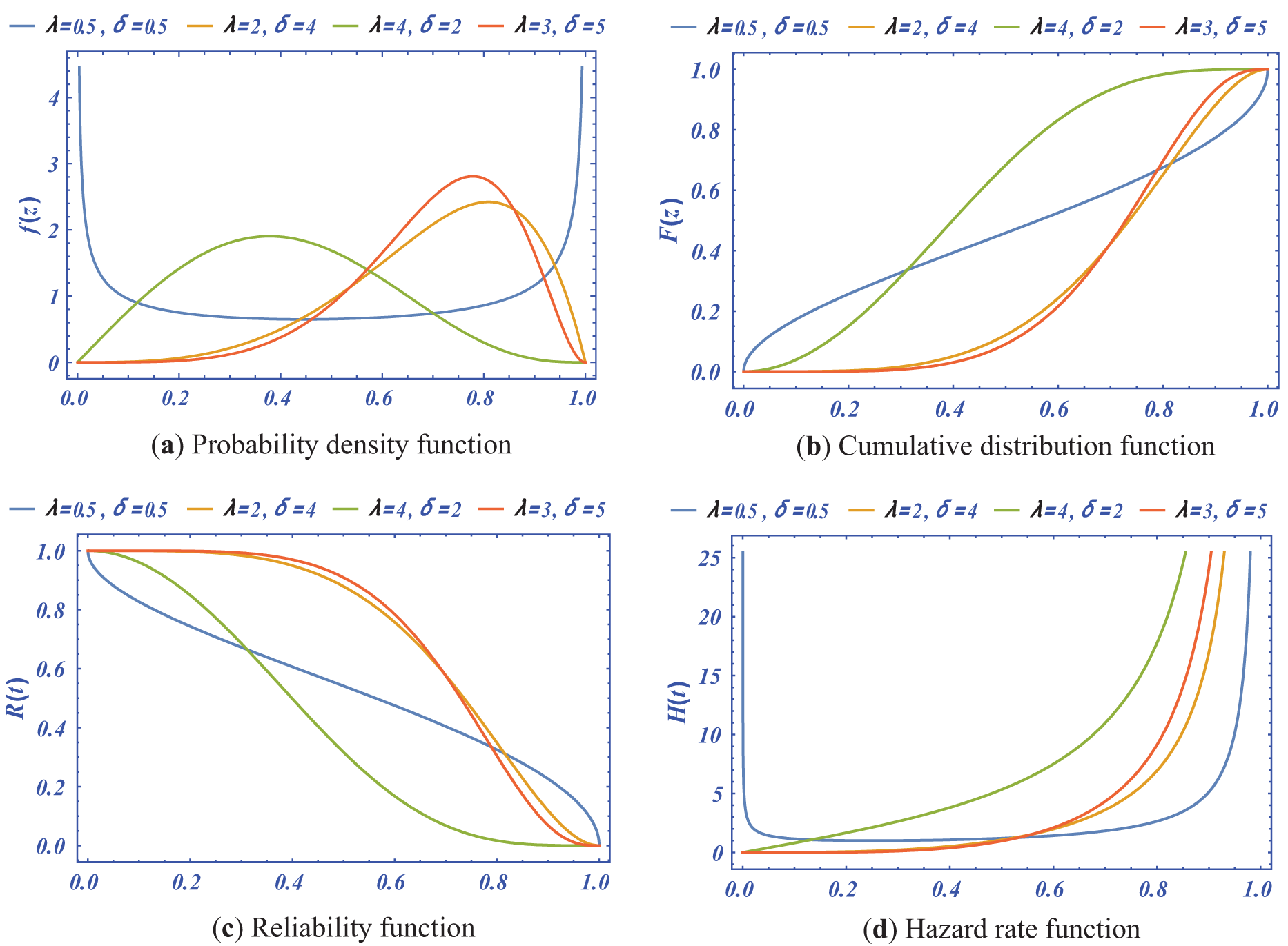
Figure 1: The PDF, CDF, RF and HRF for the Kumaraswamy distribution with different values of shape and scale parameters

Due to time, cost, and resource limitations, quality assessments that use lifetime data may encounter issues in practice. To address these problems, censoring schemes (CSs) have been employed. The progressive censoring schemes (PCSs) technique has become the norm due to its versatility and the range of data it provides. PCS states that in an experiment on experimental units, the surviving items are randomly selected from surviving items at the moment of the first failure in the test. Also, at the moment of the second failure in the test, surviving items are randomly selected from surviving items. The procedure keeps going until the failure time; at the th failure, every last surviving item is arbitrarily eliminated from the experiment. The ordered observed failure times will be designated by and referred to as progressively censored samples of size from a sample of size with PCS . The use of PCS is often motivated by practical considerations, such as cost constraints or limited resources, where it may not be feasible or efficient to monitor the subjects continuously or until the failure occurs. Data analysis using PCS poses challenges as the censoring mechanism relies on observed failure times, which may be long, and the time intervals between successive observations may vary. This requires the development of specialized statistical methods for estimation and inference. A generalized progressive hybrid censored scheme (GPHCS) was recently presented by Cho et al. [11]. He may handle the complete test duration inside the allocated time after determining the proper total test time T. Fig. 2 shows the three different cases of GPHCS.

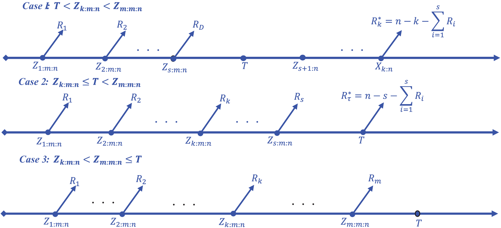
Figure 2: The Layout representation of generalized progressive hybrid censoring scheme

In the recent years, GPHCS has gained a lot of attention in reliability and survival analysis. Based on GPHCS from various distributions, Bayesian estimation has been studied by Nagy et al. in [12,13], and Nagy et al. in [14].

Bayesian estimation involves updating prior beliefs with observed data to obtain a posterior distribution. In expected Bayesian (E-Bayesian), we impose certain restrictions on our hyperparameters; it provides more stable and reliable estimates, especially in situations with uncertainty about the appropriate prior specification. The hierarchical Bayesian (H-Bayesian) method is more robust because it entails a two-stage process for constructing the prior distribution. However, a drawback of this approach lies in the intricate integrals within the estimator expression. These integrals often necessitate resolution through numerous numerical approximation techniques, making calculations tedious and time-consuming.

In the recent past, E- and H-Bayesian estimations have been considered for the parameters and the reliability characteristics under different censored data. Han [15] discussed the E-Bayesian and H-Bayesian estimations of the parameter derived from the Pareto distribution under different loss functions. Okasha et al. [16] discussed the E-Bayesian estimation for geometric distribution. Yousefzadeh [17] considered the E- and H-Bayesian estimates for Pascal distribution. Rabie et al. [18] discussed the Bayesian and E-Bayesian estimation methods of the parameter and the reliability function of the Burr-X distribution based on a generalized Type-I hybrid censoring scheme. Yaghoobzadeh [19] conducted research on E-Bayesian and H-Bayesian estimation of a scalar parameter in the Gompertz distribution under type-II censoring schemes based on fuzzy data. Their study focused on developing estimation techniques that account for uncertainty and imprecision in the data. Nassar et al. [20] conducted research on E-Bayesian estimation and associated properties of the simple step-stress model for the exponential distribution based on type-II censoring. Their study focused on developing estimation methods that account for the censoring scheme employed and investigating the properties of the estimated parameters. Nagy et al. [21] provided an E-Bayesian estimation for an exponential model based on simple step stress with Type I hybrid censored data. They developed estimation methods to obtain reliable parameter estimates considering the specific censoring scheme employed. Balakrishnan et al. [22] discussed the best linear unbiased estimation (BLUE) and maximum likelihood estimation (MLE) techniques for exponential distributions under general progressive type-II censored samples. They provided statistical methodologies for parameter estimation under this type of censoring scenario. They developed methodologies to analyze this specific censoring scheme and its impact on the estimation of the distribution’s parameters. Mohie El-Din et al. [23] proposed an E-Bayesian estimation approach for the parameters and HRF of the Gompertz distribution using type-II PCS. Their research aimed to provide reliable estimation techniques for this specific censoring scheme and demonstrated the application of these methods in practical scenarios.

Recent research has demonstrated that E- and H-Bayesian estimates are more effective than both classical and Bayesian approaches. To the best of our knowledge, no article can be found in the literature having both E- and H-Bayesian estimation for the Kumaraswamy distribution under GPHCS. Motivated by the effectiveness of E- and H-Bayesian estimates, the usefulness of the GPHCS, and the importance of the Kumaraswamy distribution in reliability applications. Our main objective in this paper is to estimate the shape parameter and the HRF of the Kumaraswamy distribution based on GPHCS using E-Bayesian and H-Bayesian approaches, which we believe would be of profound interest to applied statisticians and quality control engineers.

The structure of the article is as follows: Section 1 provides an introduction, outlining the research problem and objectives. Section 2 focuses on the MLE and Bayesian estimation techniques for the shape parameter and HRF, considering different loss functions. Section 3 presents the derivation of E-Bayesian estimators for the shape parameter under different loss functions. In Section 4, H-Bayesian estimators are obtained, again considering different loss functions. To assess the performance of the estimators, a simulation study is conducted in Section 5, where different loss functions are considered and the estimators are compared. Section 6 presents the analysis of a real-life data to demonstrate the practical application of the proposed estimators. In Section 7, the article concludes by summarizing the key findings and implications of the study. Finally, the properties of the E- and H-Bayesian estimators are discussed in the Appendix A of this paper.

2  Maximum Likelihood and Bayesian Estimation

In this section, we estimate the shape parameter and HRF of the Kumaraswamy distribution using the MLE method. Let where , for simplicity of notation, be the ordered observed failure times based on GPHCS follow from absolutely continuous PDF and RF , the joint PDF is given by

(5)

.

where is the th value of the vector .

(6)

and is the number of units eliminated at time T, as determined by

(7)

Let be the observed ordered data under the GPHCS follow from the Kumaraswamy distribution with PDF and RF as in Eqs. (1) and (3), the likelihood function of can be derived by Eq. (5), as

(8)

where and D . Taking log of Eq. (8), we get

We differentiate the above equation with respect to and equating to zero, as

(9)

The ML estimate of for given is given as

(10)

2.1 Bayesian Estimation

In calculating statistical inference and estimation of scale parameters using the Bayesian method, this is done through integrations of non-closed formulas. Then, calculating the inference and estimation of these parameters using the E- and H-Bayesian approaches is a more complex integral formula. Therefore, methods are used to approximate these quantities, which often lead to large errors. Therefore, in this manuscript, we calculate the estimate of the shape parameter for the Kumaraswamy distribution because the Bayesian estimate of this parameter is a closed form. Therefore, calculating the estimates using the E- and H-Bayesian approaches is more accurate and efficient. Here, we have developed Bayesian estimators for the shape parameter and the HRF of the Kumaraswamy distribution using various loss functions. These loss functions include the squared error loss function (SELF), entropy loss function (ELF), weighted balance loss function (WBLF), and minimum expected loss function (MELF).

We are using gamma distribution as the prior distribution of as it is a conjugate prior. The gamma prior distribution with shape and scale parameters and , respectively, has the following PDF:

(11)

Here the hyper-parameters and have been chosen based on a formula, which can be found in Dutta et al. [24]. Using the likelihood function and the prior in Eq. (11), the posterior distribution for the parameter becomes

(12)

where and we will write it as for simplicity of notation.

2.2 Bayesian Estimate with SELF

The Bayes estimator of under the squared error loss function (SELF) , is given by

(13)

provided if exists and finite. Then, by using Eqs. (12) and (13) with the sample , the Bayes estimator of under SELF is given by

(14)

The Bayes estimate of for given is given as

(15)

2.3 Bayesian Estimate with ELF

Dey et al. [25] discussed the ELF and the Bayes estimator of under ELF , is given by

(16)

provided if exists and finite. Then, by using Eqs. (12) and (16) with the sample , the Bayes estimator of under ELF is given by

(17)

The Bayes estimate of for given under ELF is given as

(18)

2.4 Bayesian Estimate with WBLF

The WBLF can be expressed as (see Nasir et al. [26]) where the Bayes estimator of under WBLF , is given by

(19)

provided if E[ and E[ exist and finite. Then, by using Eqs. (12) and (19) with the sample , we have

Hence, the Bayes estimator of under WBLF is given by

(20)

The Bayes estimate of for given under WBLF is given as

(21)

2.5 Bayesian Estimate with MELF

Tummala et al. [27] defined the MELF where the Bayes estimator of under WBLF , is given by

(22)

provided that E[ and exist and finite. Then, by using Eqs. (12) and (22) with the sample , we have

Hence, by using MELF, the Bayes estimate is obtained as

(23)

The Bayes estimate of for given under MELF is given as

(24)

3  E-Bayesian Estimation

According to Han [28], it is recommended to select the prior parameters and in such a way that the prior distribution in Eq. (11) is a decreasing function of .

Specifically, it is suggested that for and , the prior distribution becomes a decreasing function of . The E-Bayesian estimate of is given by

The E-Bayesian estimate of is then given by the integral of the Bayesian estimate of , denoted as , multiplied by the prior distribution, over suitable domains for the hyper parameters and . The domains for the first and second integrals correspond to the regions where the prior density function is a decreasing function of .

The specific distributions chosen for the hyper parameters and are as follows:

(25)

(26)

and

(27)

3.1 E-Bayesian Estimation under SELF

For a sample of the Kumaraswamy distribution, using the Bayesian estimator of under SELF in Eq. (14) with the priors given in Eqs. (25)–(27), the E-Bayesian estimators of under SELF are given by

(28)

For a time with Eq. (15), using the priors given in Eqs. (25)–(27), the E-Bayesian estimators of under SELF are given by

(29)

where and we will write it as for simplicity of notation.

3.2 E-Bayesian Estimation under ELF

For a sample from the Kumaraswamy distribution, using the Bayesian estimator of under SELF in Eq. (17) with the priors given in Eqs. (25)–(27), the E-Bayesian estimators of under ELF are given by

(30)

For a time with Eq. (18), using the priors given in Eqs. (25)–(27), the E-Bayesian estimators of under ELF are given by

(31)

3.3 E-Bayesian Estimation under WBLF

For a sample from the Kumaraswamy distribution, using the Bayesian estimator of under WBLF in Eq. (20) with the priors given in Eqs. (25)–(27), the E-Bayesian estimators of under WBLF are given by

(32)

For a time with Eq. (21), using the priors given in Eqs. (25)–(27), the E-Bayesian estimators of under WBLF are given by

(33)

3.4 E-Bayesian Estimation under MELF

For a sample of the Kumaraswamy distribution, using the Bayesian estimator of under MELF in Eq. (23) with the priors given in Eqs. (25)–(27), the E-Bayesian estimators of under MELF are given by

(34)

For a time with Eq. (24), using the priors given in Eqs. (25)–(27), the E-Bayesian estimators of under MELF are given by

(35)

4  H-Bayesian Estimation

In this part, the H-Bayesian estimates of the shape parameter of the Kumaraswamy distribution are obtained using different loss functions, namely SELF, ELF, WBLF, and MELF. Following the methodology proposed by Lindley et al. [29], we introduce hyper parameters denoted as a and b in the prior distribution Prior as given in Eq. (11). The hyper prior distributions of and are defined in Eqs. (25)–(27). Then the corresponding hierarchical prior distributions of are derived based on these hyper priors.

(36)

(37)

and

(38)

Using Bayes theorem, likelihood function and Eqs. (36)–(38), the hierarchical posterior distributions of can be written as

and

4.1 H-Bayesian Estimation Based on SELF

Using SELF and the H-posterior distributions which are defined respectively in Eqs. (13), (36)–(38), the H-Bayesian estimates , , of can be defined as

Here,

(39)

For a time , the H-Bayesian estimators of under SELF are given by

(40)

4.2 H-Bayesian Estimation Based on ELF

Using ELF and the H-posterior distributions which are defined respectively in Eqs. (16), (36)–(38), the H-Bayesian estimates , , of can be defined as

Here,

(41)

For a time , the H-Bayesian estimates of under ELF are given by

(42)

4.3 H-Bayesian Estimation Based on WBLF

Assuming WBLF as defined in Eq. (19) and using the priors defined in Eqs. (36)–(38), the H-Bayes estimates , , of are

Here,

(43)

For a time , the H-Bayesian estimates of under WBLF are given by

(44)

4.4 H-Bayesian Estimation Based on MELF

Assuming MELF as defined in Eq. (22), and using the priors defined in Eqs. (36)–(38), the H-Bayesian estimates , , of are

Then, we get

(45)

Also, the H-Bayesian estimates of under MELF are given by

(46)

In the Appendix A of this paper, we review the properties of E-Bayesian and H-Bayesian estimators of parameter and HRF .

5  Simulation Study

In this section, Monte Carlo simulation study is performed to compare the performance of the proposed estimates based on GPHCS for the Kumaraswamy distribution. The simulation study has been conducted using the R software. To generate the data, the initial true values of and are assumed as and , and k = 1. Here, the value of HRF is considered. In this simulation study, GPHCS data from Kumaraswamy distribution for a given sets of , , , , , , , , , ., ., . have been generated by using the following three progressive scheme:

•   Scheme 1: for all ;

•   Scheme 2: if is odd and if is even;

•   Scheme 3: if is odd and if is even.

The GPHCS has been generated by using the algorism in Nagy et al. [13]. Using gamma prior, the Bayes, E-Bayes and H-Bayes estimates are obtained under four different loss functions, as SELF, ELF, WBLF, and MELF. For these gamma priors, the hyperparameters is considered as . The performance of the proposed estimates has been assessed using the values of the average estimates (AEs) and the values of the mean squared error (MSE). Tables 1–4 show the values of AE and MSE for parameter , while Tables 5–8 show the values of AE and MSE for HRF . From the tables, the following conclusions have been made:

•   As the values of , , and T increases, the MSE decreases.

•   The Bayesian, E-Bayesian and H-Bayesian estimates outperform MLE in terms of MSE.

•   For any fixed loss function, the E-Bayesian estimates have smaller MSE than the Bayesian and H-Bayesian estimates.

•   For fixed value of , when or T increases, AEs come closer to their true value.

•   In most of the cases, the estimates under ELF performs better than the estimates using other loss functions.

•   In most cases, Scheme 3 have minimum mean square error compared to Schemes 1 and 2 at the same time T.

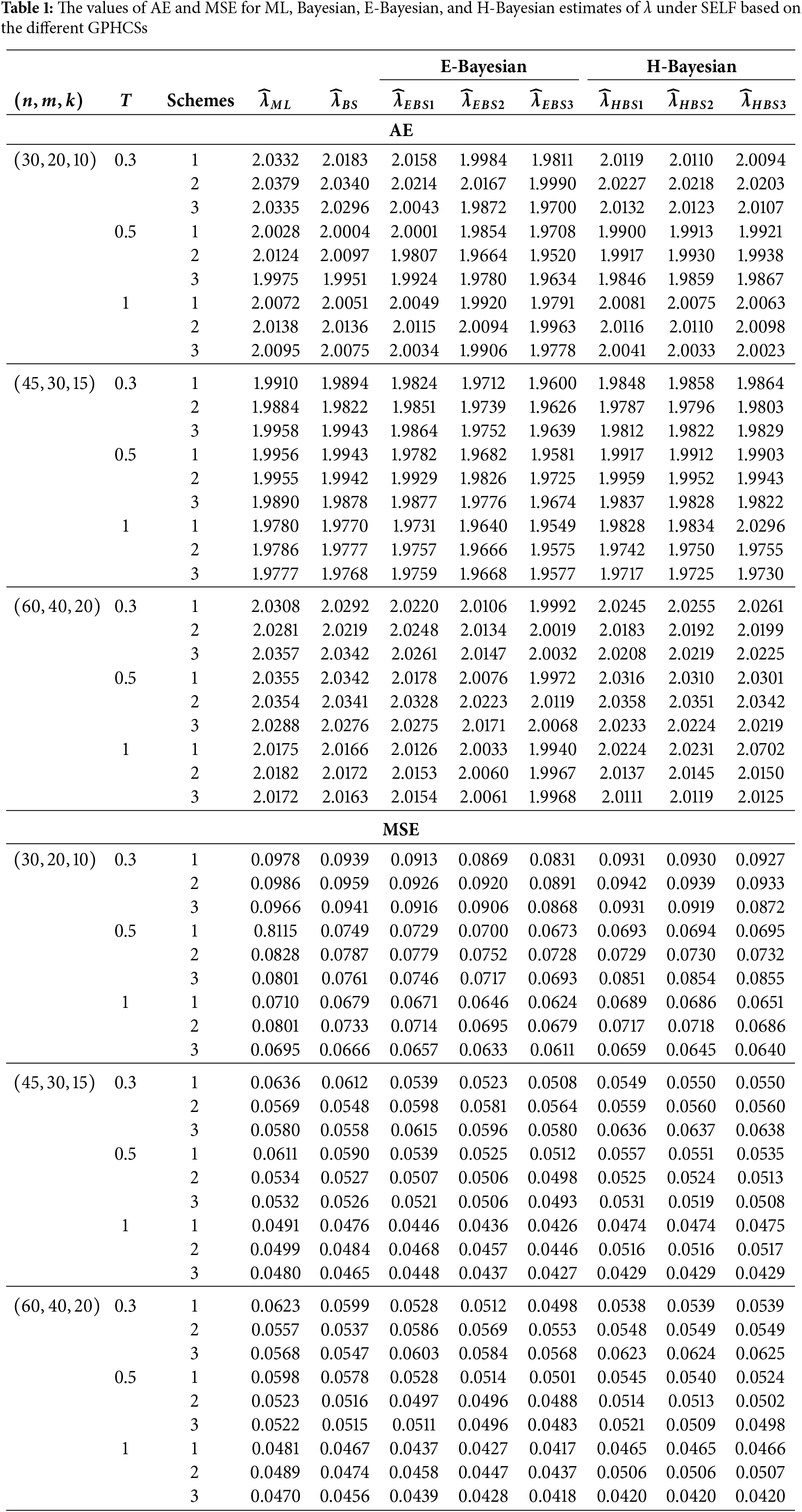
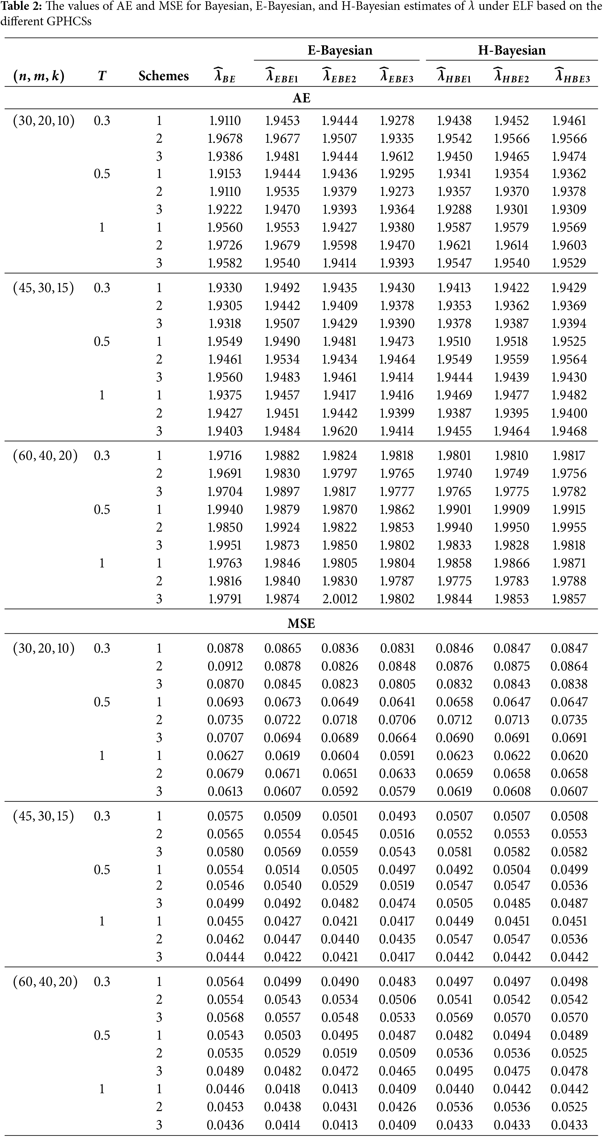
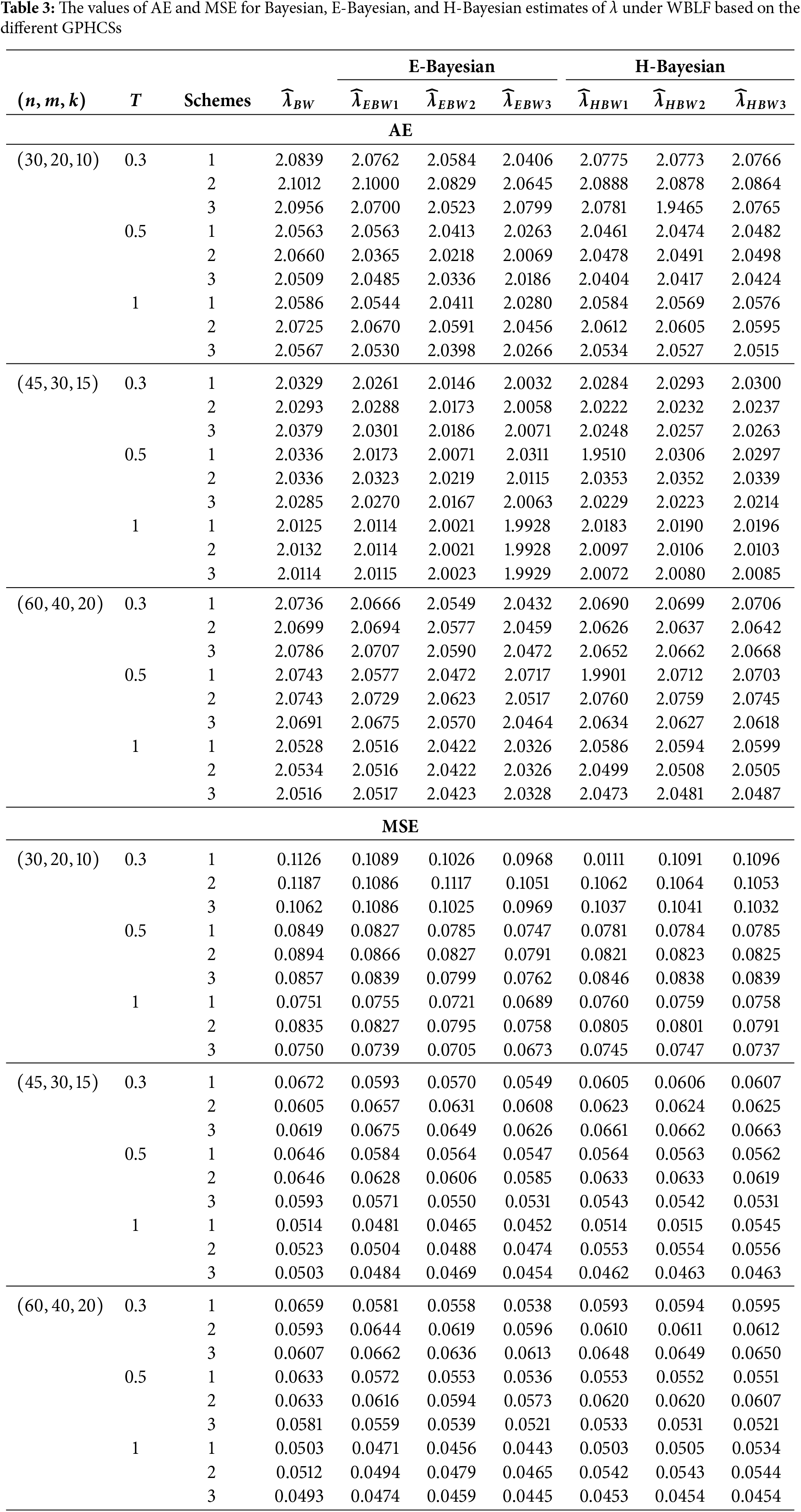
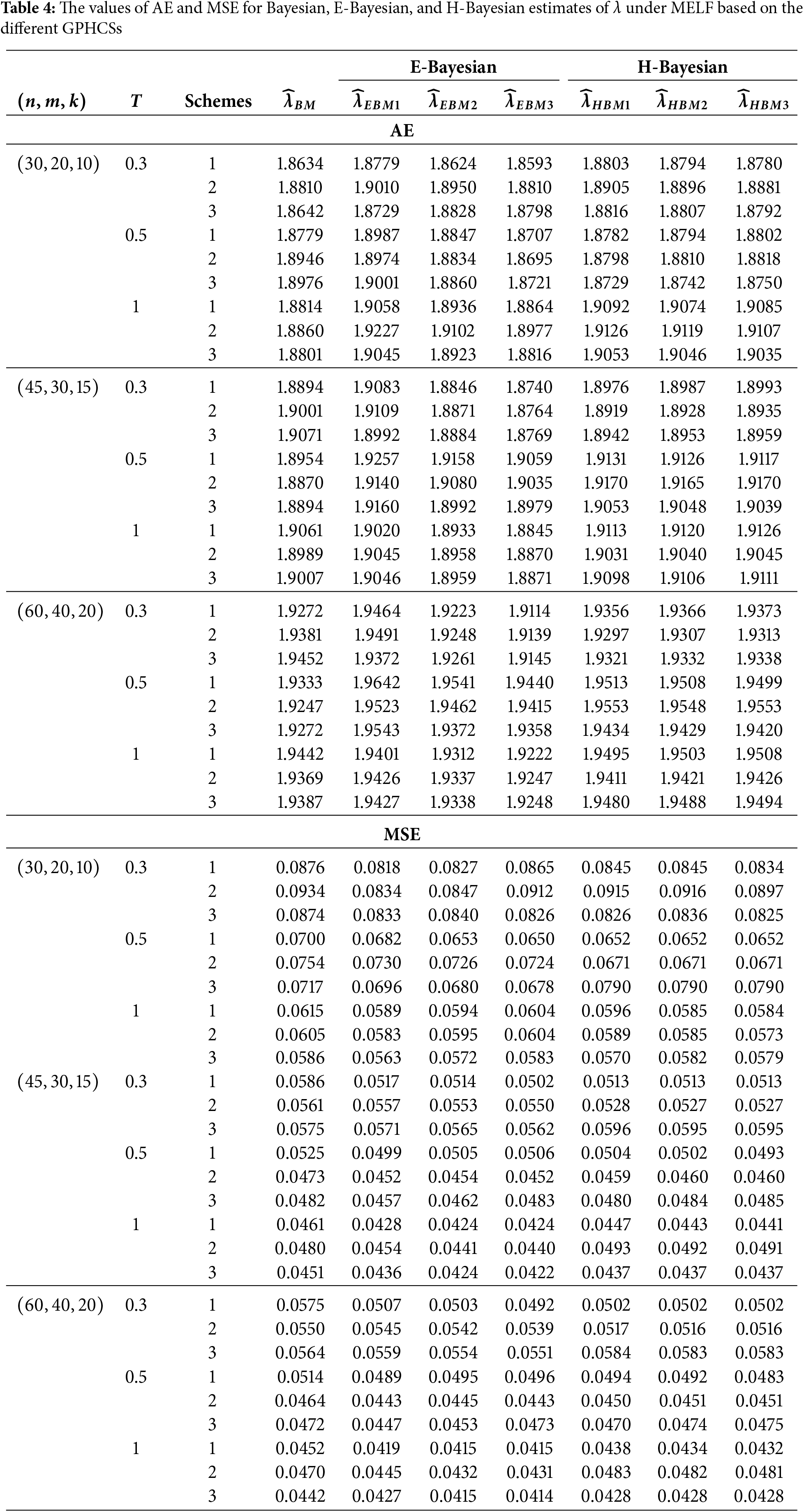
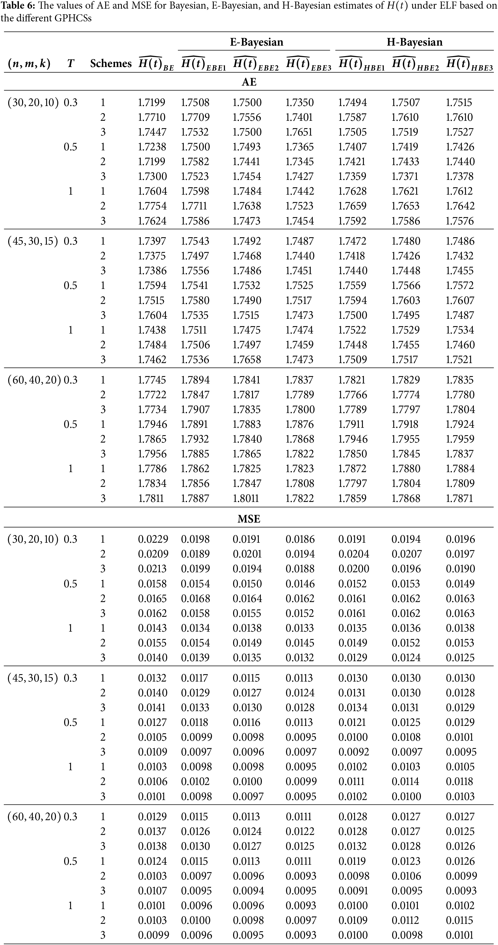
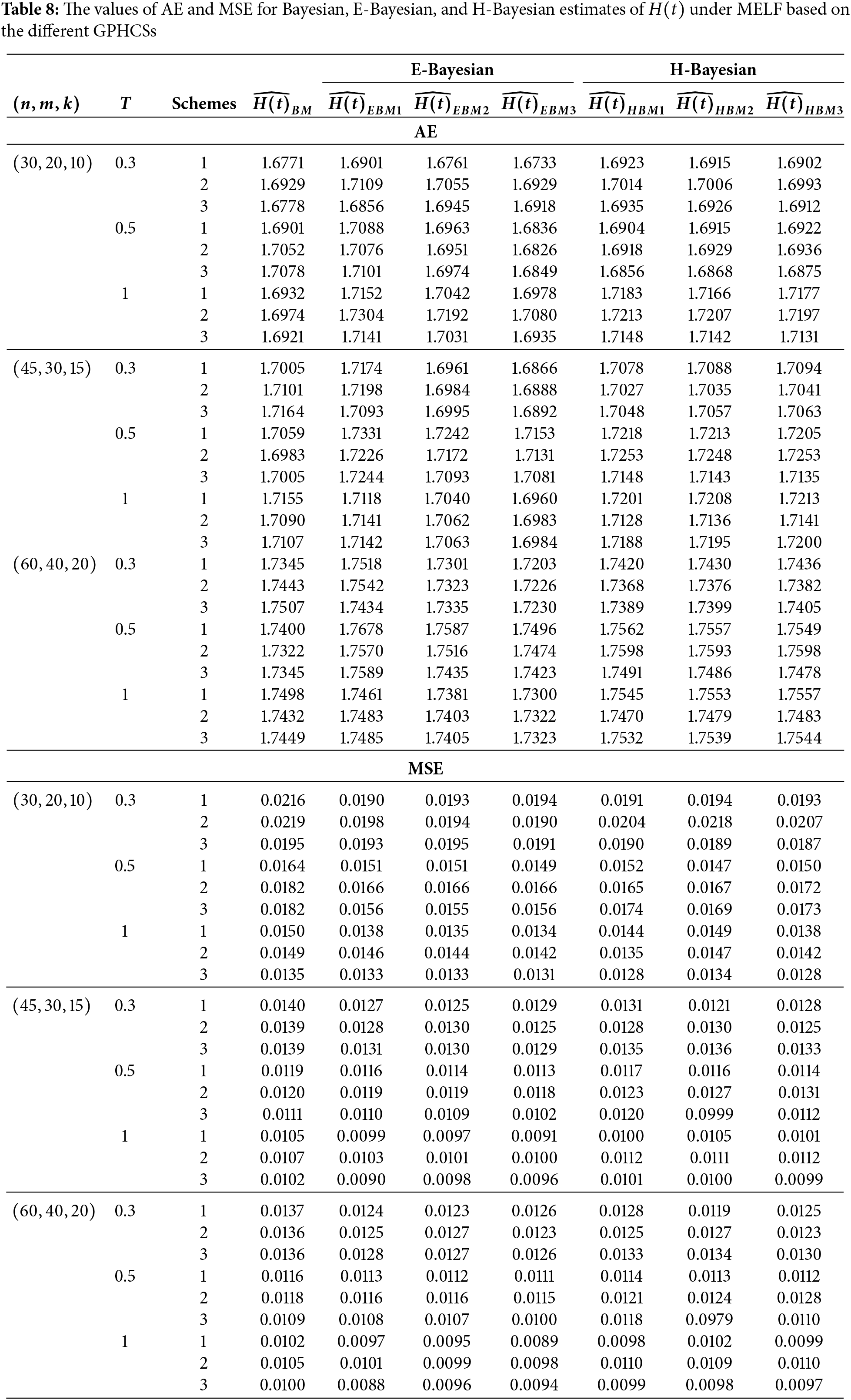
Combining all the above results, it is recommended to use the E-Bayesian technique to estimate the parameters and the HRF for GPHCS based on ELF, due to the better performance than other estimates in terms of MSE.

6  Applications to Real Data

This section uses a real-world dataset as an example to analyze the applicability of the suggested estimation techniques. The following dataset, which spans the years 1975 to 2016, displays the monthly water capacity of the Shasta reservoir between the months of August and December. Some statisticians, including Kohansal [30] and Tu et al. [31], have previously exploited these data. We shall use these data to consider the following PCS: Suppose , , , and different values of , , and , with R using as the following three different PCS,

•   Scheme 1: for all , ,…, and ;

•   Scheme 2: if is odd and if is even;

•   Scheme 3: if is odd and if is even.

Table 9 shows the ML, Bayesian, E-Bayesian, and H-Bayesian estimates for the unknown parameter and HRF based on the GPHCS.

7  Conclusions

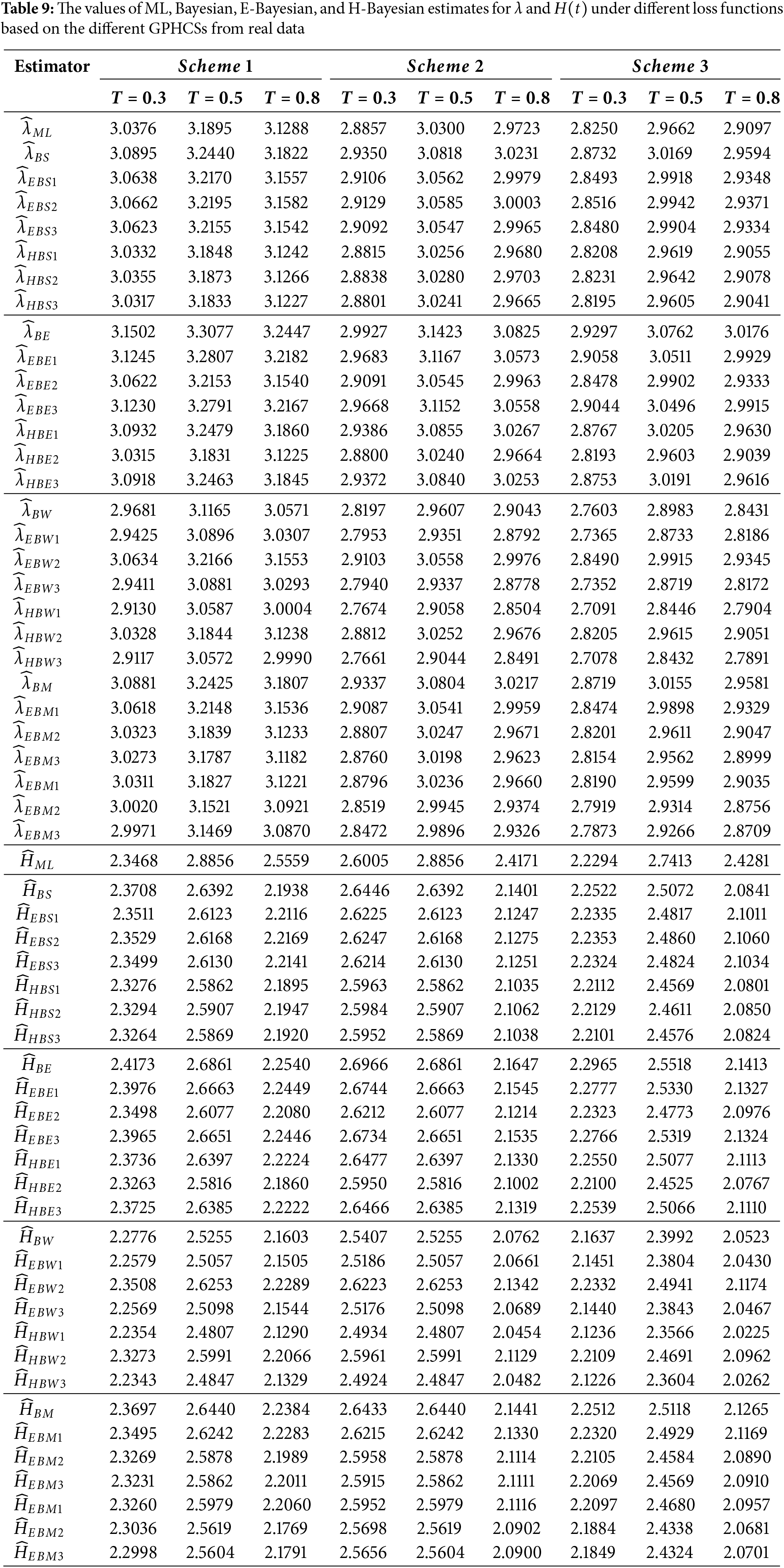
This paper proposes E-Bayesian and H-Bayesian estimations using GPHCS for the unknown shape parameter and HRF of the Kumaraswamy distribution. To obtain the Bayesian, E- and H-Bayesian estimates, the squared error, entropy, weighted balance, and minimum expected loss functions are introduced. A Monte Carlo simulation study has been performed to compare the performance of the estimates of parameters such as the shape parameter and HRF. In terms of AE and MSE, the simulation study yields that E-Bayesian estimates outperform all other estimates. Finally, a real data set has been analyzed to illustrate the applicability of the proposed estimates. After analyzing this data, it is concluded that E-Bayesian estimates for the parameters and the HRF perform better than other estimates; the sample size as well as the observed sample size are very important factors for determining the efficiency of the estimators. The E- and H-Bayesian estimation approach for the scale parameter and reliability function of the Kumaraswamy under GPHCS using different loss functions is done through more complex integral formulas so that it is interesting and difficult work that needs more time. We are currently addressing this problem as part of our future research.

Acknowledgement: The author is grateful to the editor and anonymous referees for their insightful comments and suggestions, which helped to improve the paper’s presentation. The author extends his appreciation to King Saud University for funding this work through Researchers Supporting Project, King Saud University, Riyadh, Saudi Arabia.

Funding Statement: This research was funded by Researchers Supporting Project number (RSPD2025R969), King Saud University, Riyadh, Saudi Arabia.

Availability of Data and Materials: The data was mentioned along the paper.

Ethics Approval: The author declares that this study don’t include human or animal subjects.

Conflicts of Interest: The author declares no conflicts of interest to report regarding the present study.

Appendix A Properties of E-Bayesian and H-Bayesian Estimation of λ: In this section, the properties of E-Bayesian estimates and the relations among the E-Bayesian and H-Bayesian estimates are discussed.

Appendix A.1 The Relations between the E-Bayesian Estimates under Different Loss Functions

Theorem A1: It follows from Eq. (28) that

(1)

(2)

(3)

Proof: (1) From Eq. (28), we have

and

Therefore,

For , we have .

Let , when , , we get

where . Thus,

which yields that, .

(2) From (1), we get

So it can be easily obtained that .

(3) From Eq. (28) and from the proof of (1), we have

Using (2), we get , j = 1, 2, 3.

Theorem A2: It follows from Eq. (30) that

(1)

(2) ,

(3)

Proof: (1) From Eq. (30), we have

and

Therefore,

For , we have . Let , when , , we get

where . Thus,

which yields that, .

(2) From (1), we get

So it can be easily obtained that .

(3) From Eq. (30) and from the proof of (1), we have

Using (2), we get , j=1, 2, 3.

Theorem A3: It follows from Eq. (32) that

(1) ,

(2) ,

(3)

Proof: (1) From Eq. (32), we have

and

Therefore,

For , we have Let , when , , we get

Then,

This shows that

(2) From (1), we get

This yields that,

From Eq. (32) and from the proof of (1), we have Using (2), we get , for .

Theorem A4: It follows from Eq. (34) that

(1)

(2)

(3)

Proof: (1) From Eq. (34), we have

and

For , we have

Let , when , , we get

where .

Thus,

(A1)

That is .

From (1), we get

(A2)

That is, .

From Eq. (34) and from the proof of (1), we have . Using (2), we get , j = 1, 2, 3.

Similar relationships holds for the E-Bayesian estimates of under different loss functions.

Appendix A.2 The Relations between the H-Bayesian Estimates under Different Loss Functions

Theorem A5: It follows from Eq. (39) that , for .

Proof: Based on SELF, the H-Bayesian estimate of can be expressed as

Using the result , we have

As , and For , , is continuous and and, hence, using the generalized mean value theorem, we can find at least one number and such that

Therefore,

Taking limit as , it has been noticed that, . Similarly, we have . Thus, , for .

Theorem A6: It follows from Eq. (41) that , for .

Proof: Based on ELF, the H-Bayesian estimate of can be expressed as

Using the result , we have

As , and For , , is continuous and and, hence, using the generalized mean value theorem, we can find at least one number and such that

Therefore,

Taking limit as , it has been noticed that, . Similarly, we have . Thus, , for .

Theorem A7: It follows from Eq. (43) that , for

Proof: Under WBLF, the H-Bayesian estimate of can be expressed as

Using the result, , we have

As , and For , , is continuous and and, hence, using the generalized mean value theorem, we can find at least one number and such that

Therefore,

(A3)

Taking limit as , it has been obtained that . Similarly, we have Thus, for .

Theorem A8: It follows from Eq. (45) that

Proof: Under MELF, the H-Bayesian estimate of can be expressed as

Using the result , we have

As , and For , , is continuous and and, hence, using the generalized mean value theorem, we can find at least one number and such that

(A4)

Taking limit as Similarly, we have Thus, .

Similar relationships holds for the H-Bayesian estimates of HRF under different loss functions.

References

1. Kumaraswamy P. A generalized probability density function for double-bounded random processes. J Hydrol. 1980;46(1–2):79–88. doi:10.1016/0022-1694(80)90036-0. [Google Scholar] [CrossRef]

2. Sundar V, Subbiah K. Application of double bounded probability density function for analysis of ocean waves. Ocean Eng. 1989;16(2):193–200. doi:10.1016/0029-8018(89)90005-X. [Google Scholar] [CrossRef]

3. Fletcher SG, Ponnambalam K. Estimation of reservoir yield and storage distribution using moments analysis. J Hydrol. 1996;182(1–4):259–75. doi:10.1016/0022-1694(95)02946-X. [Google Scholar] [CrossRef]

4. Mitnik PA. New properties of the Kumaraswamy distribution. Commun Statistcs-Theory Methods. 2013;42(5):741–55. doi:10.1080/03610926.2011.581782. [Google Scholar] [CrossRef]

5. Ponnambalam K, Seifi A, Vlach J. Probabilistic design of systems with general distributions of parameters. Int J Circuit Theory Appl. 2001;29(6):527–36. doi:10.1002/cta.173. [Google Scholar] [CrossRef]

6. Dey S, Mazucheli J, Nadarajah S. Kumaraswamy distribution: different methods of estimation. Comput Appl Math. 2018;37(2):2094–111. doi:10.1007/s40314-017-0441-1. [Google Scholar] [CrossRef]

7. Jamal F, Arslan Nasir M, Ozel G, Elgarhy M, Mamode Khan N. Generalized inverted Kumaraswamy generated family of distributions: theory and applications. J Appl Stat. 2019;46(16):2927–44. doi:10.1080/02664763.2019.1623867. [Google Scholar] [CrossRef]

8. Alshkaki R. A generalized modification of the Kumaraswamy distribution for modeling and analyzing real-life data. Statist, Optim Inform Comput. 2020;8(2):521–48. doi:10.19139/soic-2310-5070-869. [Google Scholar] [CrossRef]

9. Mahto AK, Lodhi C, Tripathi YM, Wang L. Inference for partially observed competing risks model for Kumaraswamy distribution under generalized progressive hybrid censoring. J Appl Stat. 2022;49(8):2064–92. doi:10.1080/02664763.2021.1889999. [Google Scholar] [PubMed] [CrossRef]

10. Alduais FS, Yassen MF, Almazah MM, Khan Z. Estimation of the Kumaraswamy distribution parameters using the E-Bayesian method. Alex Eng J. 2022;61(12):11099–110. doi:10.1016/j.aej.2022.04.040. [Google Scholar] [CrossRef]

11. Cho Y, Sun H, Lee K. Exact likelihood inference for an exponential parameter under generalized progressive hybrid censoring scheme. Stat Methodol. 2015;23:18–34. doi:10.1016/j.stamet.2014.09.002. [Google Scholar] [CrossRef]

12. Nagy M, Sultan KS, Abu-Moussa MH. Analysis of the generalized progressive hybrid censoring from Burr Type-XII lifetime model. AIMS Math. 2021;6(9):9675–704. doi:10.3934/math.2021564. [Google Scholar] [CrossRef]

13. Nagy M, Bakr ME, Alrasheedi AF. Analysis with applications of the generalized type-II progressive hybrid censoring sample from burr type-XII model. Math Probl Eng. 2022;2022(1):1241303. doi:10.1155/2022/1241303. [Google Scholar] [CrossRef]

14. Nagy M, Alrasheedi AF. The lifetime analysis of the Weibull model based on Generalized Type-I progressive hybrid censoring schemes. Math Biosci Eng. 2022;19(3):2330–54. doi:10.3934/mbe.2022108. [Google Scholar] [PubMed] [CrossRef]

15. Han M. The E-Bayesian and hierarchical Bayesian estimations of Pareto distribution parameter under different loss functions. J Stat Comput Simul. 2017;87(3):577–93. doi:10.1080/00949655.2016.1221408. [Google Scholar] [CrossRef]

16. Okasha HM, Wang J. E-Bayesian estimation for the geometric model based on record statistics. Appl Math Model. 2016;40(1):658–70. doi:10.1016/j.apm.2015.05.004. [Google Scholar] [CrossRef]

17. Yousefzadeh F. E-Bayesian and hierarchical Bayesian estimations for the system reliability parameter based on asymmetric loss function. Commun Statist-Theory Methods. 2017;46(1):1–8. doi:10.1080/03610926.2014.968736. [Google Scholar] [CrossRef]

18. Rabie A, Li J. E-Bayesian estimation for Burr-X distribution based on generalized type-I hybrid censoring scheme. Am J Math Manag Sci. 2020;39(1):41–55. doi:10.1080/01966324.2019.1579123. [Google Scholar] [CrossRef]

19. Yaghoobzadeh Shahrastani S. Estimating E-bayesian and hierarchical bayesian of scalar parameter of gompertz distribution under type II censoring schemes based on fuzzy data. Commun Stat–Theory Methods. 2019;48(4):831–40. doi:10.1080/03610926.2017.1417438. [Google Scholar] [CrossRef]

20. Nassar M, Okasha H, Albassam M. E-Bayesian estimation and associated properties of simple step-stress model for exponential distribution based on type-II censoring. Qual Reliab Eng Int. 2021;37(3):997–1016. doi:10.1002/qre.2778. [Google Scholar] [CrossRef]

21. Nagy M, Abu-Moussa M, Alrasheedi AF, Rabie A. Expected Bayesian estimation for exponential model based on simple step stress with Type-I hybrid censored data. Math Biosci Eng. 2022;19(10):9773–979. doi:10.3934/mbe.2022455. [Google Scholar] [PubMed] [CrossRef]

22. Balakrishnan N, Sandhu RA. Best linear unbiased and maximum likelihood estimation for exponential distributions under general progressive type-II censored samples. Sankhyã: Indian J Stat, Ser B. 1996;58(1):1–9. [Google Scholar]

23. Mohie El-Din MM, Sharawy A, Abu-Moussa MH. E-Bayesian estimation for the parameters and hazard function of Gompertz distribution based on progressively type-II right censoring with application. Qual Reliab Eng Int. 2023;39(4):1299–317. doi:10.1002/qre.3292. [Google Scholar] [CrossRef]

24. Dutta S, Kayal S. Estimation and prediction for Burr type III distribution based on unified progressive hybrid censoring scheme. J Appl Stat. 2024;51(1):1–33. doi:10.1080/02664763.2022.2113865. [Google Scholar] [PubMed] [CrossRef]

25. Dey D, Gosh M, Srinivasan C. Simultaneous estimation of parameters under entropy loss. J Stat Plan Inference. 1986;15:347–63. doi:10.1016/0378-3758(86)90108-4. [Google Scholar] [CrossRef]

26. Nasir W, Aslam M. Bayes approach to study shape parameter of Frechet distribution. Int J Basic Appl Sci. 2015;4(3):246. doi:10.14419/ijbas.v4i3.4644. [Google Scholar] [CrossRef]

27. Tummala VMR, Sathe PT. Minimum expected loss estimators of reliability and parameters of certain lifetime distributions. IEEE Trans Reliab. 1978;27(4):283–5. doi:10.1109/TR.1978.5220373. [Google Scholar] [CrossRef]

28. Han M. The structure of hierarchical prior distribution and its applications. Chin Oper Res Manag Sci. 1997;6(3):31–40. [Google Scholar]

29. Lindley DV, Smith AF. Bayes estimates for the linear model. J Royal Statist Soc Series B: Statist Methodol. 1972;34(1):1–18. doi:10.1111/j.2517-6161.1972.tb00885.x. [Google Scholar] [CrossRef]

30. Kohansal A. On estimation of reliability in a multicomponent stress-strength model for a Kumaraswamy distribution based on progressively censored sample. Stat Pap. 2019;60(6):2185–224. doi:10.1007/s00362-017-0916-6. [Google Scholar] [CrossRef]

31. Tu J, Gui W. Bayesian inference for the Kumaraswamy distribution under generalized progressive hybrid censoring. Entropy. 2020;22(9):1032. doi:10.3390/e22091032. [Google Scholar] [PubMed] [CrossRef]