SL-COA: Hybrid Efficient and Enhanced Coati Optimization Algorithm for Structural Reliability Analysis

1  Introduction

With the increasing complexity of engineering structures, structural reliability analysis (SRA) plays an increasingly important role in engineering design, operation, and maintenance. Traditional structural reliability analysis methods, while capable of obtaining relatively accurate results, suffer from extremely low computational efficiency when faced with small failure probabilities or large-scale finite element analyses. Therefore, the development of efficient and accurate structural reliability analysis methods has become a research hotspot. This study aims to address this challenge by improving existing optimization algorithms and combining them with the first-order reliability method (FORM) to propose a new structural reliability analysis framework for solving reliability analysis problems in complex engineering structures. This research not only has significant theoretical value but also boasts broad application prospects, providing engineers with more reliable and efficient analysis tools for engineering design.

SRA is not only beneficial to the systematic adjustment of structural safety factors but also a key factor in structural design and operation maintenance [1–3]. SRA plays a very important role in preventing higher-level risks in the life expectancy of engineering structures [4,5]. Higher-level risks in engineering structures can include catastrophic failures, such as bridge collapses, building collapses, and aircraft crashes. For example, the collapse of the I-35W Mississippi River bridge in Minneapolis in 2007 resulted in significant loss of life and property damage [6]. Reliability analysis can help prevent such failures by ensuring that engineering structures are designed to withstand expected loads and environmental conditions with high reliability. At the same time, it can also help engineers design more safe and reliable mechanical systems [7–10].

SRA is usually performed by calculating or estimating the probability that the research object violates the limit state function (LSF) during its life cycle [11,12]. Monte Carlo simulation (MCS) is a very important tool in the field of SRA, which has been widely studied based on the original MCS [13]. In addition, the use of analytical methods to complete SRA has also been widely studied. Common analytical methods include FORM [14], second-order reliability method (SORM) [15], first-order second-moment (FOSM) [16] and so on. Compared with using MCS to complete SRA, the analytical method requires lower computational cost. While analytical methods such as FORM generally require lower computational costs compared to MCS for low-dimensional problems, they face significant limitations in high-dimensional problems. This is because the complexity of the reliability analysis increases exponentially with the number of dimensions. In high-dimensional spaces, analytical methods may struggle to find the Most Probable Point (MPP) efficiently, leading to increased computational costs and potential inaccuracies. Furthermore, the assumptions made in analytical methods, such as local linear approximations of the LSF, may become less valid in high-dimensional spaces, further compromising the accuracy of the results. Although the use of MCS to complete structural reliability analysis can obtain a more accurate failure probability or reliability index. However, with the increasing complexity of engineering structures, the computational efficiency of MCS is very low in the face of engineering examples with small failure probability or large-scale finite element analysis [17,18]. Therefore, the subset simulation (SS) method [19], importance sampling (IS) method [20], and line sampling (LS) [21] method have been developed. In addition, the use of surrogate models instead of simulation or complex constraint functions has a very effective effect on reducing the number of assessments of limit states. Common surrogate models include the Kriging model [22–24], polynomial chaos expansion (PCE) [25], response surface method (RSM) [26], artificial neural network (ANN) [27], or support vector regression (SVR) method [28,29]. However, in the face of high-dimensional problems, it may be impossible to establish a reliable alternative model for SRA [30,31] due to overfitting or underfitting. Relatively speaking, the accuracy of the surrogate model-assisted hybrid reliability analysis method depends largely on the reliability of the surrogate model and the selection of training sample points [32,33]. However, the accuracy of the analytical reliability method depends more on searching the MPP, that is, the point [34,35] with the smallest distance from the origin in the standard normal space. This makes the calculation cost required in the process of reliability analysis by analytical method relatively lower. Therefore, this study mainly considers the FORM.

In recent years, researchers have continued to refine and expand the capabilities of FORM. Zhang et al. [36] proposed an enhanced finite step length (EFSL) method to improve the efficiency and robustness of solving complex nonlinear reliability-based design optimization (RBDO) problems. Yang et al. [37] proposed an efficient local adaptive Kriging approximation method with a single-loop strategy (LAKAM-SLS) to enhance the computational efficiency of Kriging-based RBDO. These developments aim to enhance the accuracy, efficiency, and robustness of FORM, particularly in addressing the challenges posed by complex and high-dimensional engineering structures. By incorporating these recent advancements, the field of SRA is continuously evolving, striving to provide more reliable and efficient methods for assessing structural safety and preventing catastrophic failures.

In the past few years, researchers have done a lot of research on SRA based on analytical methods. Among them, the traditional MPP search methods include the gradient method or conjugate gradient method. Although for low-dimensional reliability analysis problems, traditional FORM often obtains stable and accurate analysis results. Studies have shown that the relaxed Hasofer–Lind and Rackwitz–Fiessler (RHL-RF) [38], and non-negative constraint method (NNCM) [39] are inefficient in solving nonlinear convex LSFs [40]. These methods often face the problem of over-reliance on parameter settings or non-convergence of results. In addition, the convex problem may also be a big challenge for gradient FORM, and its computational cost may increase significantly in some solving processes. The meta-heuristic algorithm can obtain accurate results or close to the exact solution, which avoids the problem that the gradient method cannot obtain the reliability analysis solution due to the inability to converge [41,42].

As a non-gradient optimization algorithm, the meta-heuristic algorithm solves the optimization problem by simulating biological behavior or physical processes [43]. At present, there have been many studies on heuristic algorithm-assisted FORM. Zhu et al. [40] proposed an improved particle swarm optimization (PSO) algorithm-assisted FORM. The results show that the new FORM has higher stability and computational efficiency in the solution of MPP for complex problems. Pedroso [44] combines a typical differential evolution algorithm with FORM. From the calculation results, it can be seen that it has a very good performance in finite element examples that require large-scale simulation. Zhong et al. [45] proposed a new Harris Hawk optimization algorithm (HHO). The combination of the HHO algorithm and FORM improves the efficiency and stability of solving MPP points in high-dimensional examples. In FORM, the most critical issues of non-gradient search include. 1) The accuracy and robustness of MPP search; 2) Improve the reliability analysis ability of complex engineering structure models. If the simulation strategy is difficult or even impossible to obtain effective reliability analysis results, FORM can provide acceptable analysis results with low computational difficulty; 3) Improve the computational efficiency of FORM for complex reliability analysis problems. It is still important to develop a meta-heuristic algorithm with higher global convergence performance and faster convergence efficiency, which plays an important role in improving the efficiency, accuracy, and stability of searching MPP points.

Coati optimization algorithm (COA) [46] is a heuristic optimization algorithm, which has been proved to have good global development and local search capabilities. At the same time, it is also an optimization algorithm that does not need to apply any parameters to control. However, in the process of solving MPP, problems such as inaccurate calculation results or low computational efficiency may still be encountered. In this study, the social learning strategy is used to improve the COA (SL-COA), aiming to improve computational efficiency, global convergence ability, and robustness of the algorithm. By testing the benchmark test sets CEC2005 and CEC2017 and four optimization design examples, the SL-COA algorithm is demonstrated to improve the convergence speed and robustness. Secondly, this study combines the SL-COA algorithm with FROM to construct a reliability analysis method. Finally, the applicability and effectiveness of the SL-COA algorithm in the field of reliability analysis are verified by four mathematical examples and two engineering examples.

The rest of the paper is structured as follows: In Section 2, the knowledge of FORM and COA is briefly introduced. Then, in Section 3, the proposed SL-COA and the novel framework are explained in detail. In Section 4, both mathematical and engineering examples are conducted to test the effectiveness of the enhanced COA and proposed hybrid reliability analysis framework, and then their results are fully discussed. Ultimately, Section 5 provides a conclusion and prospects for this study.

2  Review of Related Knowledge

2.1 First-Order Reliability Method

SRA plays an important role in evaluating the safety and reliability of engineering structures under load and degradation. Estimating the failure probability based on a specific LSF is the most important goal of SRA [40]:

(1)

where denotes the LSF, denotes the joint probability density function (PDF) of n-dimensional random variable set . Because of the difficulty of solving the integral, researchers have proposed a method to solve the approximate solution close to the accurate reliability index by searching MPP. As shown in Fig. 1, a schematic diagram for searching MPP in a certain probability space is given.

Figure 1: Schematic representation mixed model in the U-space

2.1.1 First-Order Reliability Method Based on Gradient

Eqs. (2) and (3) give the calculation formula of MPP point and reliability index by gradient method. This method is a reliability analysis method that combines the design point search based on an iterative gradient with the local linear approximation of the LSF in the standard normal probability space.

(2)

(3)

where denotes the normalized sensitivity vector. Furthermore, . The iterative formulas of different gradient reliability analysis methods are different. The element in is , which denotes the normal standard random variable. Eq. (4) gives the calculation formula of .

(4)

where

(5)

(6)

where, and denotes the cumulative distribution function (CDF) and the PDF of original variable . The calculation of is the most important difference between different gradient reliability analysis methods, for example:

1). Hasofer–Lind and Rackwitz–Fiessler method (HL-RF) [38].

HL-RF is one of the most classic forms. The iterative formula of this method is given by Eq. (7).

(7)

2). Conjugate HL-RF algorithm [2]

To improve the performance of HL-RF, researchers proposed a conjugate HL-RF algorithm. can be computed as follows:

(8)

where can be computed by Eq. (9).

(9)

where . The calculation formula of conjugate gradient vector is shown as Eq. (10).

(10)

where . With the help of scalar factor , no longer coincides with the sensitivity vector of the previous iteration, reducing the periodicity risk.

3). Finite step length method (FSL) [36]

The radial sensitivity vector in FSL is calculated by Eq. (11).

(11)

where is bigger than 0. In the iterative process, the calculation formula is the same as that shown in Eq. (9). The iterative instability of highly nonlinear LSF is controlled by changing factor .

2.1.2 First-Order Reliability Method Based on Heuristic Algorithm

The computational efficiency and stability of the gradient-based FORM are good for low and nonlinear reliability analysis problems. However, in the face of moderate nonlinear problems and moderate dimensional reliability problems, acceptable reliability analysis results may not be obtained. The heuristic algorithm is very effective in obtaining acceptable reliability analysis results for complex problems. By transforming the reliability analysis problem into the following Eq. (12):

(12)

where denotes the fitness function. denotes the LSF. is the penalty factor [5]. It can be seen from Eq. (12) that the method improves the efficiency of solving the reliability index by solving the MPP in the failure domain.

Fig. 2 shows the calculation flow of the first-order reliability method using the heuristic algorithm.

Figure 2: First-order reliability method flow based on the heuristic algorithm

Step 1: Initialize the heuristic algorithm and initialize the relevant parameters.

Step 2: Build the fitness function based on the reliability analysis problem by Eq. (12).

Step 3: A heuristic optimization algorithm is used to optimize the fitness function.

Step 4: Use the Eq. (13) to determine whether the current optimization results are accurate. is used in the current study. If the current optimization result does not satisfy Eq. (13), implement Step 5; Otherwise, Step 6 is implemented.

(13)

Step 5: Update related parameters such as the penalty factor and return to Step 2.

Step 6: Output the current reliability analysis result.

2.2 Coati Optimization Algorithm

The batch normalization (BN) layer is an optimization method widely used in deep neural networks proposed by Ioffe [47] aiming to improve the training speed of models and reduce the impact of gradient vanishing and exploding problems. The BN layer normalizes the inputs between network layers, giving them zero mean and unit variance, thereby enhancing training stability. In CNNs, BN layers are typically inserted between convolutional layers and activation function layers. The COA is a novel metaheuristic algorithm introduced by Dehghani in 2022 [46]. It sets up a mathematical model to mimic the behavior of coati in nature. The basic idea of COA is the simulation of the two natural behaviors of coatis:

     i)  Capturing and pursuing iguanas,

    ii)  Evasion of potential threats.

Correspondingly, the execution process of COA is elucidated and mathematically represented in two distinct phases: exploration and exploitation.

Initialization: The initial positions of the coatis in the search space are randomly set using:

(14)

where is the position of the ith coati in search space, is the value of the jth decision variable, is the number of coatis, is the number of decision variables, is a random real number between 1 and 2, and and are the lower bound and upper bound of the jth decision variable, respectively. After initialization, the individual coati starts to perform the two phases.

Phase 1: Hunting strategy (exploration phase)

The initial stage of population adjustment among the coatis within the search space involves simulating their behaviors when facing iguana attacks. It is assumed that half of the coatis choose to climb the tree, while the other half opt to stay on the ground, anticipating the iguana’s descent. This methodology encourages coatis to migrate to different positions within the search space, highlighting the ability of COA to explore the entire problem-solving domain globally.

Climbing Coatis: It is postulated that the best member of the population occupies the position of the iguana. Therefore, the position of the coatis rising from the tree is mathematically simulated using Eq. (15).

For

(15)

where is the new position calculated for the ith coati, is the value of its jth dimension, is random variable in the interval , represents the iguana’s position in the jth dimension, is an integer, which is randomly selected from the set , and is the floor function.

Ground Coatis: Once the iguana descends to the ground, it is positioned at a random location within the search space. Subsequently, the coatis on the ground navigates the search space, a process replicated using Eqs. (16) and (17).

(16)

For

(17)

where represents the position of the iguana on the ground, is the value of the objective function.

If a newly calculated position for each coati improves the value of the objective function, it is considered suitable for the update process; otherwise, the coati maintains its current position. This update criterion applies to all coatis with indices , as defined by Eq. (18).

(18)

Phase 2: Escaping strategy (exploitation phase)

The second stage of updating the coati positions is mathematically structured to mirror the natural response of coatis when they encounter and evade predators. When faced with a predator’s attack, coatis adopt a strategy that leads them to a safer spot near their current position. This behavior underscores the coatis’ capacity for local search and exploiting their surroundings.

Local Position Update: To emulate this behavior, a random position is generated in close proximity to the current location of each coati, as determined by Eq. (19).

(19)

where and represent the local lower and upper bounds for the jth decision variable, and denote the lower bound and upper bound of the jth decision variable, is the iteration counter, is the new position calculated for the ith coati on the second phase of COA and is the value of its jth dimension.

Position Acceptance: The freshly computed position is considered acceptable if it enhances the value of the objective function, which is assessed using the condition expressed in Eq. (20).

(20)

where is the objective function.

One iteration of the COA is completed after updating the positions of all coatis in the search space during the first and second phases. This cycle continues until the final iteration of the algorithm is reached. At the end of the COA run, the best solution obtained throughout all iterations of the algorithm is presented as the output. The various steps involved in the COA implementation are illustrated in Fig. 3 through a flowchart.

Figure 3: Block diagram of COA

3  Improved COA-Based FORM

In this section, the proposed hybrid reliability analysis model is discussed. Firstly, the improved COA is explained, and after that, the framework of this analysis model is defined and illustrated.

3.1 Social Learning-Adapted COA

The status monitoring of the forging press machine uses 4 types of sensors, including 4 channels of displacement signals, 4 channels of impact force signals, 2 channels of hydraulic signals, and 2 channels of air pressure signals. Each set of data collected consists of one sample with 12 channels. According to the duration of approximately 8 s for each forging operation on the forging press machine, the length for each signal is set at 8000 data points with a sampling frequency of 1000 Hz.

This paper introduces a novel method for COA enhancement called SL-COA. Social learning is a basic behavior of the biotic population. In the field of swarm intelligence algorithms, this concept is initially explained in another bioinspired algorithm called PSO [48]. It is a swarm intelligence algorithm proposed by Kennedy and Eberhart in 1995, inspired by the social behavior of birds and fish. The core concept of the algorithm is as follows.

Considering a D-dimensional space consists of n particles, the velocity and position of each particle are defined as

(21)

(22)

In each iteration, the above expression is updated as

(23)

(24)

where is the velocity in dth iteration, is the best position of an individual particle, and is the best position of the whole swarm, is inertia weight and is learning factor.

This expression elucidates the concept that an individual’s velocity within a group can be characterized as a blend of influences from their prior velocity, self-awareness, and the collective influence of the group. Actually, this idea is also suitable for most of the swarm intelligence algorithms [48–51]. In this paper, this idea is used to improve the learning process of the behavior of coatis. That is the Eqs. (15), (17) and (19).

There are two types of indexes related to the swarm learning process in PSO, that is inertia weight and learning factor . The inertia weight is a parameter measured by the influence of the prior velocity of the swape. A higher value of results in less frequent velocity changes, as it diminishes the impact of velocity adjustments. The learning factor is employed to fine-tune both self-awareness and the collective impact of the group. Conversely, a greater value of leads to a more pronounced velocity change [49,50]. As for COA, the learning factor is adopted in both phases 1 and 2. It improves the convergence speed in Phase 1 and regulates the swarm diversity in Phase 2, preventing premature convergence to suboptimal solutions.

In PSO, the learning index is treated as a constant. However, it should be noticed that as the iterations progress, the disparity between each individual varies. In response to this variation, the learning index should be mathematically linked to it [49]. Consequently, a variable learning index is introduced as , where is the current iteration, is total iteration, and are the maximum and minimum learning index respectively. This expression represents that with iterations progress, the learning index gradually decreases from to .

Therefore, the updated process (Eqs. (15), (17), and (19)) of COA is changed to Eqs. (25)–(27), respectively.

(25)

(26)

(27)

The block diagram of the algorithm is shown in Fig. 4.

Figure 4: Block diagram of SL-COA

3.2 The Proposed Framework for FORM

By combining the improved algorithm with FORM, a new reliability analysis framework is constructed. The framework applies the SL-COA algorithm to the MPP search process and then converts the output results into reliability index and failure probabilities . The proposed reliability analysis framework is shown in Fig. 5.

Figure 5: Block diagram of SL-COA-based FORM framework

4  Study Case and Discussion

In the following section, the performance of the improved optimization algorithm and the proposed reliability analysis framework are tested in sequence.

4.1 Examples for Illustration

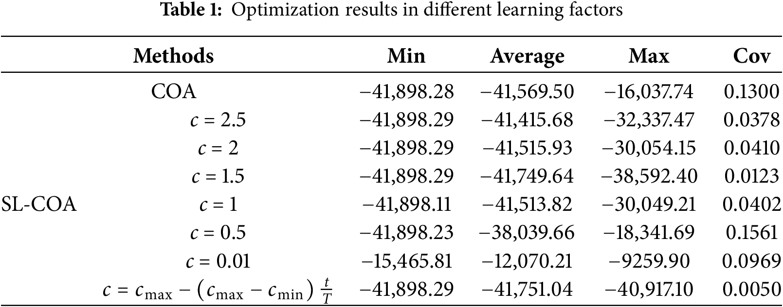
In this example, the objective function shown in Eq. (28) is optimized to compare the effects of different learning factors on the performance of the optimization algorithm SL-COA. Among them, the number of populations is set to 20, and the maximum number of iterations is set to 50.

(28)

where variable x is the normal distribution variable. The lower bound of the variable is 500. The upper bound of the variable is 500. Table 1 shows the optimization results of different learning factors c and adaptive learning factors after 50 times of optimization.

where , . It can be seen from the results in the table that the stability of the optimal solution obtained by using a fixed learning factor is relatively low. Comparing the average value of the optimal solution obtained in the repeated experiments, it can be found that the searchability of the SL-COA algorithm decreases as the learning factor c decreases. It can be seen that the optimal solution obtained by the proposed adaptive learning factor change strategy has higher accuracy and higher stability.

4.2 Examples of Optimization Procedure

The optimization performance of SL-COA is firstly evaluated under some mathematical and engineering cases. This discussion is conducted by comparing with another metaheuristic algorithm. That includes WOA (2016) [52], OOA (2023) [53], Rime Optimization Algorithm (RIME) algorithm (2023) [54], the multi-verse optimizer (MVO) (2015) [55], the tree-seed algorithm (TSA) (2015) [56] as well as its original version COA (2023) [46].

4.2.1 Mathematical Examples

Firstly, CEC2005 is used to justify the performance of the SL-COA. There are totally 25 functions in this setting: Unimodal function , Basic multimodal function , Extended multimodal function and Mixed composite function . Among these problems, are believed to have most difficulties due to its complex structure. In this section, are used to evaluate the basic optimization abilities of the proposed algorithm. The search history, trajectory curve, average curve as well as convergence curve of SL-COA is illustrated in Fig. 6. These problems vary in complexity and dimensionality, making them suitable for evaluating the performance of optimization algorithms across a wide range of scenarios.

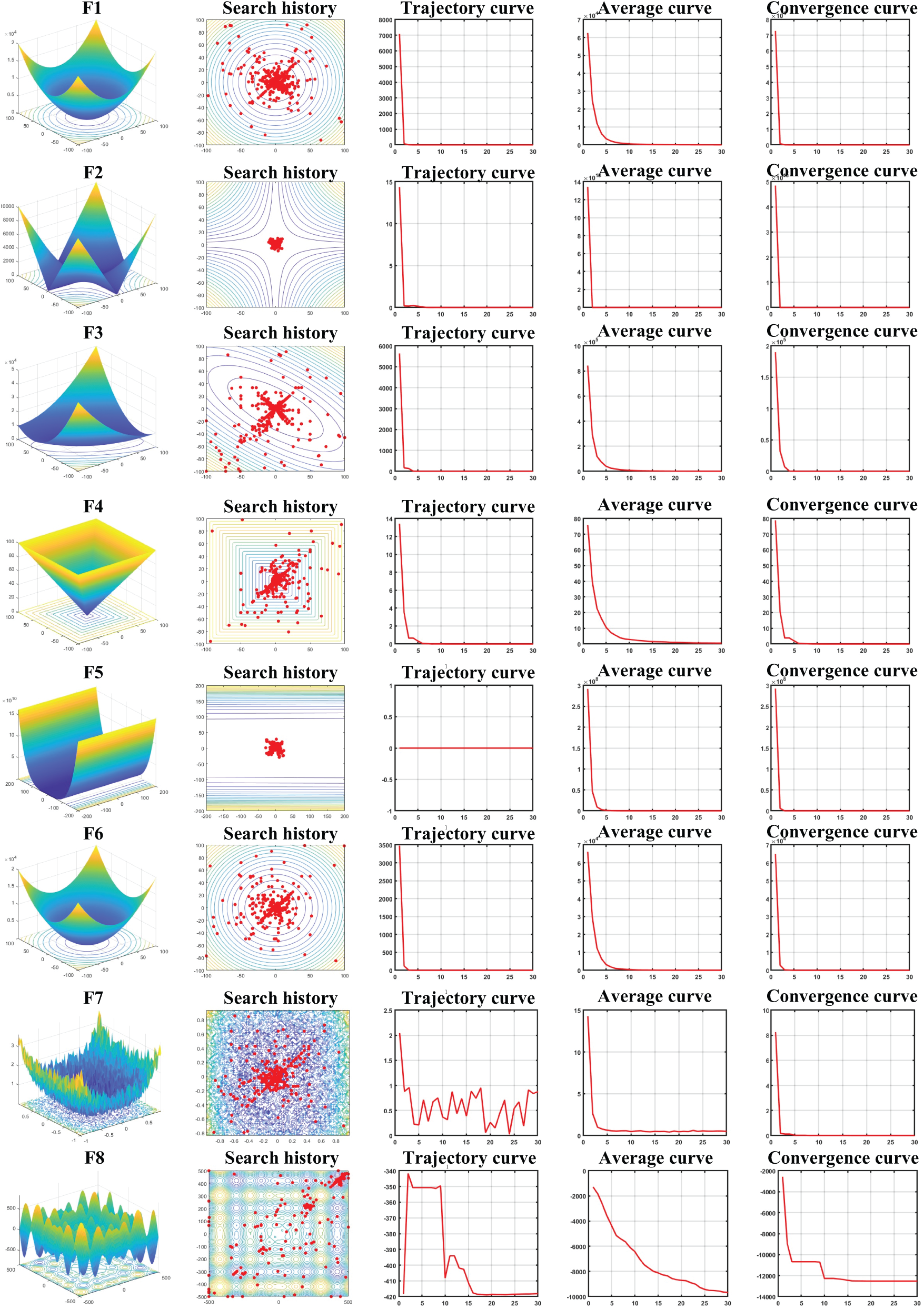
Figure 6: Test results for CEC2005

The results demonstrate that SL-COA effectively identifies optimal solutions for each function. The search history graph, which displays position swaps after each iteration, exhibits a high concentration near the optimization point in the search space. The trajectory curve, representing the fitness of the first dimension, steadily decreases as the iterations progress. It initially exhibits steep changes but tends to stabilize towards the end of the optimization process. The average curve, depicting the mean fitness of all search candidates, and the convergence curve, showcasing the best individual’s performance, collectively provides an overview of the optimization’s overall performance. It’s important to observe that when testing the proposed SL-COA under function F7, there is a fluctuation throughout the entire iteration process, as evidenced by the trajectory curve. In this case, the vertical coordinates of the trajectory curves represent the function value, and the horizontal coordinates represent the iteration number. However, this fluctuation remains within the range of [−1, 0], and considering the good performance of the entire swarm, it can be deemed acceptable on the whole.

After that, CEC2017 is used to future evaluate the performance of the optimization. The function details of this testing set is listed in Table 2. CEC2017 contains 30 optimization problems, categorized into four groups: unimodal functions, multimodal functions, hybrid functions, and composition functions. Similar to the CEC2005 test set, these problems are designed to be challenging and representative of real-world optimization problems. The CEC2017 test set includes more complex and high-dimensional problems compared to the CEC2005 test set, making it a more rigorous benchmark for evaluating the performance of optimization algorithms.

The key parameters of each algorithm are listed in Table 3. Additionally, the size of the population is set to 30, the maximum iteration number is 1000. Each function is tested 50 times, and the average, standard deviation and errors of the results are calculated.

The output results are analyzed to compute their mean value and standard deviation. Subsequently, each algorithm is assigned a ranking based on the magnitude of their errors. A comprehensive breakdown of the results can be found in the “CEC2017 Results” appendix. The sum of rankings across all functions and the mean value for each algorithm are presented in Table 4. Additionally, the convergence curve of each algorithm is shown in Fig. 7 and the box diagram illustrates the distribution of optimization results shown in Fig. 8.

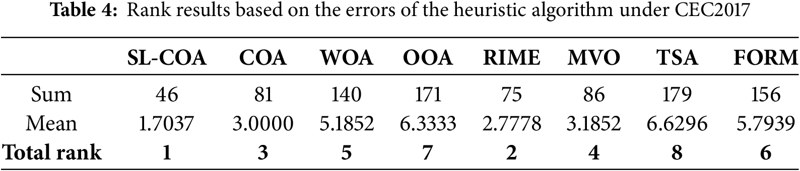
Figure 7: Convergence curve of CEC2017

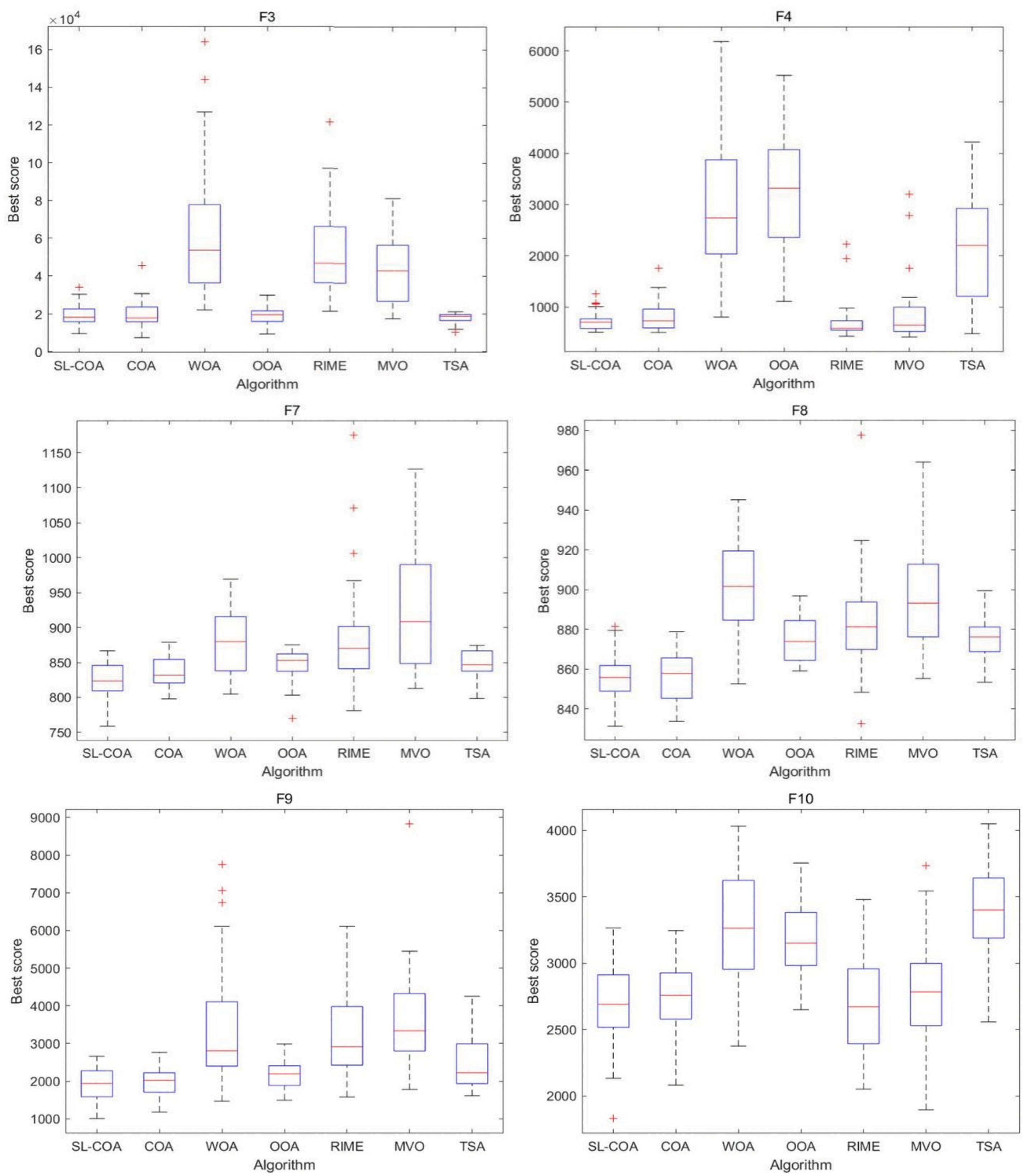
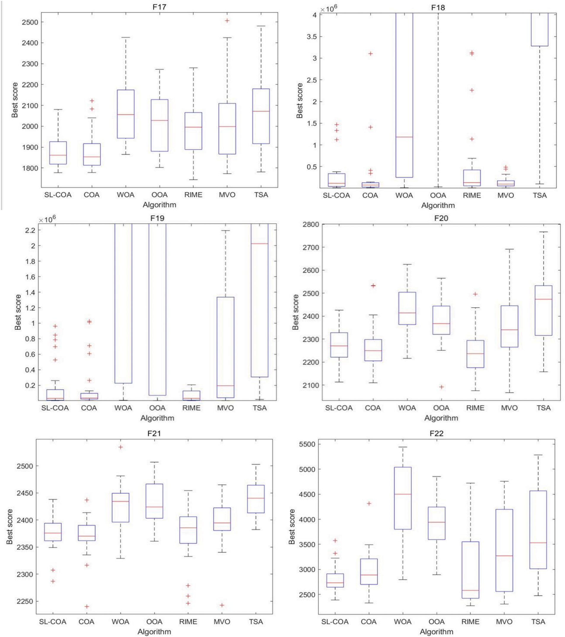
Figure 8: Box diagram of CEC2017

It could be found that SL-COA performs better on most of the functions. When comparing it to the original version (COA), it becomes evident that SL-COA offers distinct advantages for most functions, except for F10, F11, and F17. When compared to other heuristic algorithms, this algorithm demonstrates a notable superiority in terms of both average values and standard deviation. The convergence curve graphs illustrate the convergence performance of different algorithms. It can be observed that SL-COA exhibits faster convergence and effectively avoids local optima during the search process. The box graph visually displays the output distribution of the proposed algorithm, effectively illustrating both the average and standard deviation of the results.

Upon closer examination, while it’s true that RIME occasionally exhibits better performance with specific test functions, the cumulative rank sum of RIME remains significantly higher than that of SL-COA. This may be attributed to its frequent failure to address certain hybrid and composite functions. RIME is believed to have a better optimization performance than COA, however, it cannot match the proposed SL-COA overall. Additionally, it is worth noting that when tackling composition functions, SL-COA demonstrates a clear advantage. While the error in certain problems (e.g., F30) is still large, it consistently delivers superior results when compared to other algorithms for the majority of cases.

4.2.2 Engineering Examples

In this section, four examples with engineering backgrounds are tested to evaluate the performance of the SL-COA. These comparisons are also conducted between SL-COA and the six heuristic algorithms mentioned above.

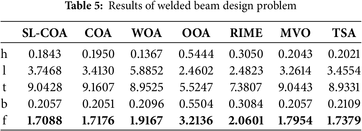
Example 1. Welded beam design problem

The objective of this problem is to find the optimal dimensions of a welded beam that minimizes the cost while satisfying certain constraints on its performance and safety (shown in Fig. 9) [57]. The design of the welded beam involves four variables: height (h), length (l), thickness (t), and width (b). The objective function to minimize is the cost of the beam, which is given by:

Figure 9: Welded bean design

Consider:

Minimize:

Subject to:

(29)

Parameter range:

where

The comparison results are listed in Table 5.

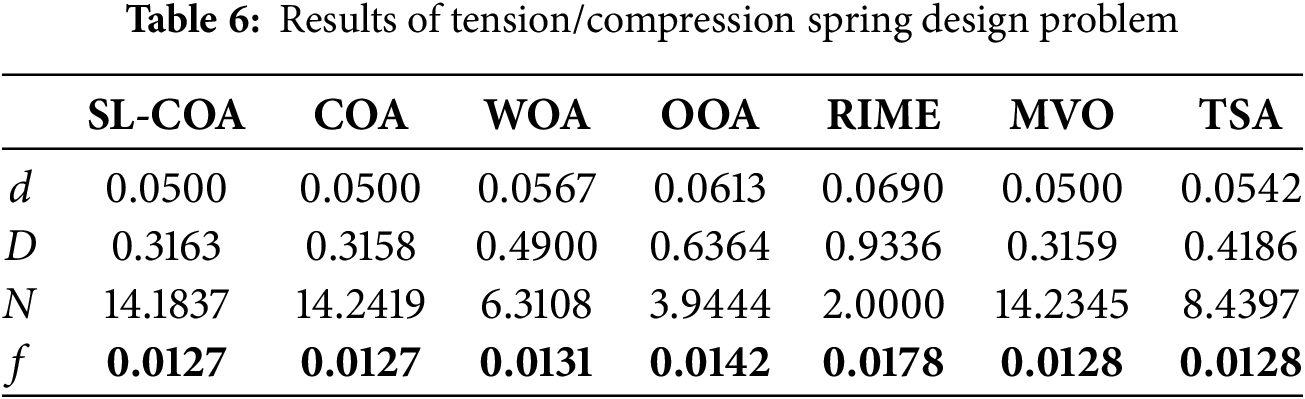
Example 2. Tension/compression spring design problem

The tension/compression spring design problem is another classical optimization problem in engineering (shown in Fig. 10) [58]. The objective of this problem is to determine the optimal dimensions and parameters of a tension or compression spring to meet certain performance requirements while minimizing manufacturing or material costs. The comparison of different algorithms is shown in Table 6.

Figure 10: Tension/compression spring design

Consider:

Minimize:

Subject to:

(30)

Parameter range:

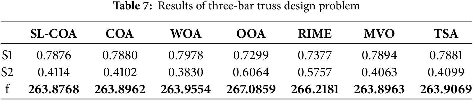
Example 3. Three-bar truss design problem

This problem involves the optimization of the dimensions and geometry of a truss structure composed of three bars (or members) and typically used to support loads or distribute forces within a structure (shown in Fig. 11) [59]. The objective is to find the optimal design that minimizes certain criteria, such as weight or cost while ensuring that the truss can support the applied loads and maintain structural stability. The results are shown in Table 7.

Figure 11: Three-bar truss design

Consider:

Minimize:

Subject to:

(31)

Parameter range:

where

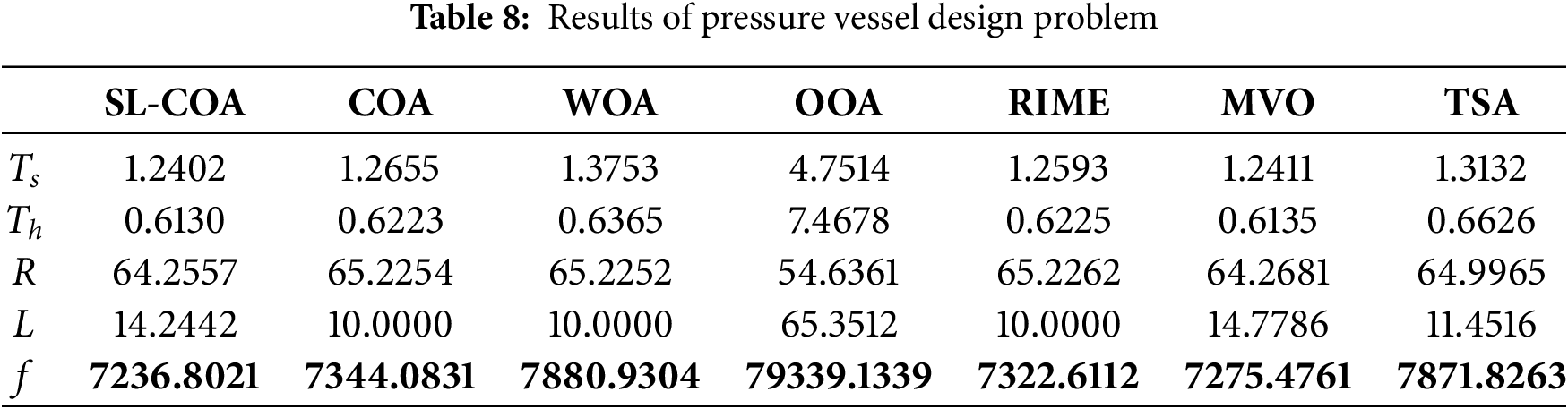
Example 4. Pressure vessel design problem

The pressure vessel design problem (show in Fig. 12) is an important engineering optimization problem related to the design and sizing of pressure vessels [60]. Pressure vessels are containers designed to hold and store fluids or gases at high pressure. They are used in various industries, including petrochemical, aerospace, and manufacturing, and must be designed to safely contain the pressurized contents while minimizing material and manufacturing costs. The results are shown in Table 8.

Figure 12: Pressure vessel design problem

Consider:

Minimize:

Subject to:

(32)

Parameter range:

It is shown that the utilization of SL-COA produces the best design for all four problems. The convergence curve is shown in Fig. 13. It is evident that SL-COA exhibits swift convergence and possesses the capability to thoroughly explore the solution space, thereby avoiding premature convergence to local optima. The number of iterations needed may vary depending on the complexity of the problems, but SL-COA consistently maintains a leading position among other algorithms. It’s worth mentioning that RIME, known for its strong performance in mathematical scenarios, no longer exhibits its advantages in this engineering context. This could be attributed to its suboptimal optimization for solving certain polynomial functions, which mirrors its performance in mathematical problems (F7, F25, F27). These findings underscore the competitive edge held by the proposed SL-COA in addressing real world engineering challenges.

Figure 13: Convergence curve of 4 engineering problems

4.3 Examples of Reliability Analysis

In this section, the proposed SL-COA-based FORM framework is evaluated by mathematical examples and engineering examples. The proposed SL-COA FORM framework is compared with the FORM based on Sequential Quadratic Programming (SQP) or other optimization algorithms. In addition, the reliability analysis results of MCS are considered to be accurate reliability analysis results, which can be used to refer to other reliability analysis results.

4.3.1 Mathematical Examples

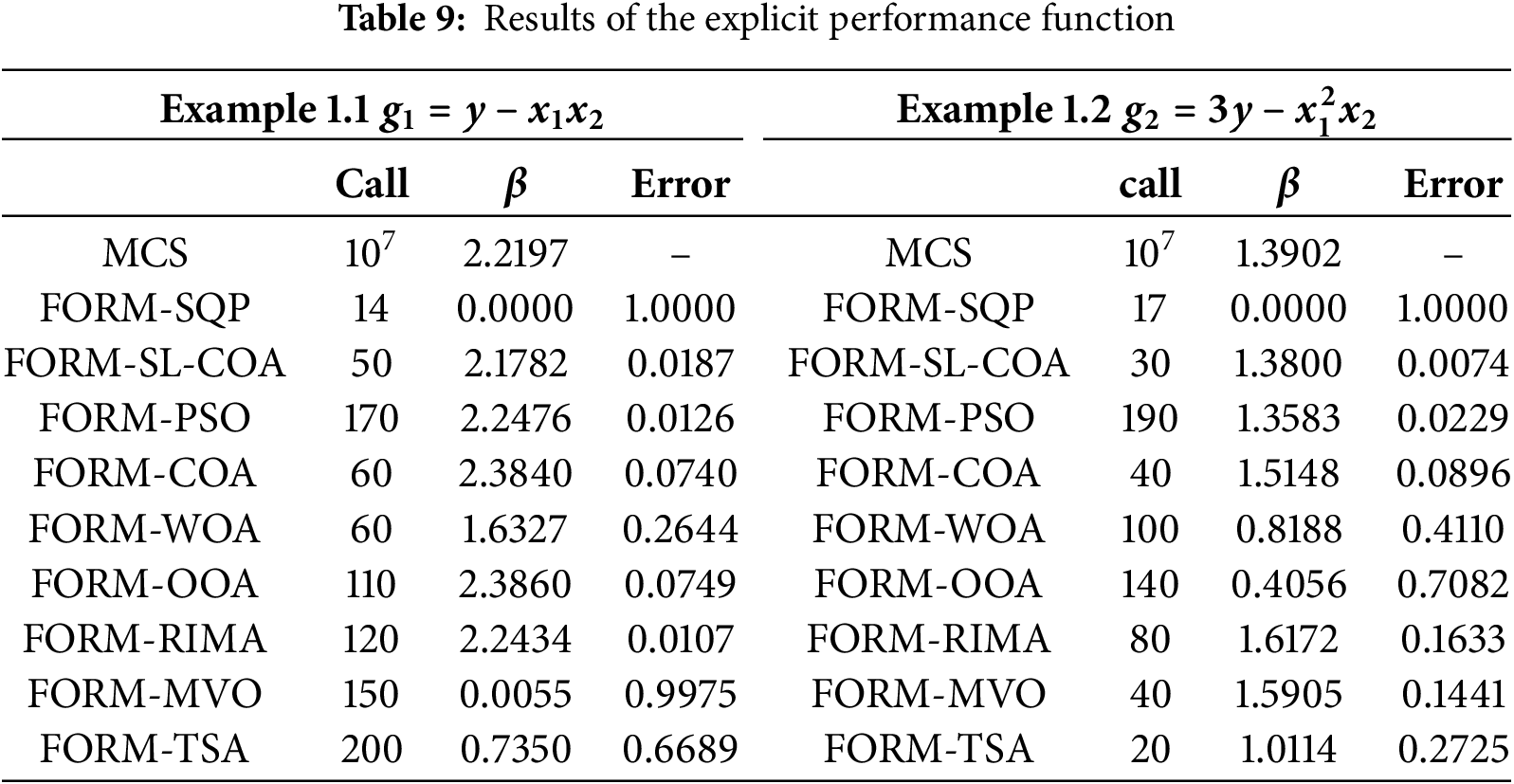
Example 1. Explicit performance function

Example 1 showcases reliability analysis problems with different explicit performance functions. Simulating the failure domain of the structural performance functions demonstrates how to effectively utilize the SL-COA algorithm to find the MPP, thereby calculating the reliability index. A mathematically straightforward problem involving three uncertain variables is tested in this section. We examine two distinct performance functions, denoted as and , and their corresponding formulations.

(33)

(34)

where and are normally distributed variables with mean values of and . The standard deviations and , respectively. The interval variable . It is obvious that . The reliability index and the number of function calls are tested. The results are shown in Table 9.

The convergence curve is shown in Fig. 14.

Figure 14: Convergence curve of Example 1

This example illustrates the effective resolution of the problem using the proposed method, which delivers high accuracy and efficient function calls. In the heuristic algorithm-based FORM, the determination of function calls occurs at the conclusion of their interactions.

In Example 1.1, the output shows the third fewest errors, yet it delivers exceptional performance in terms of the number of function calls. In Example 1.2, it yields the most precise results while utilizing the second lowest number of function calls.

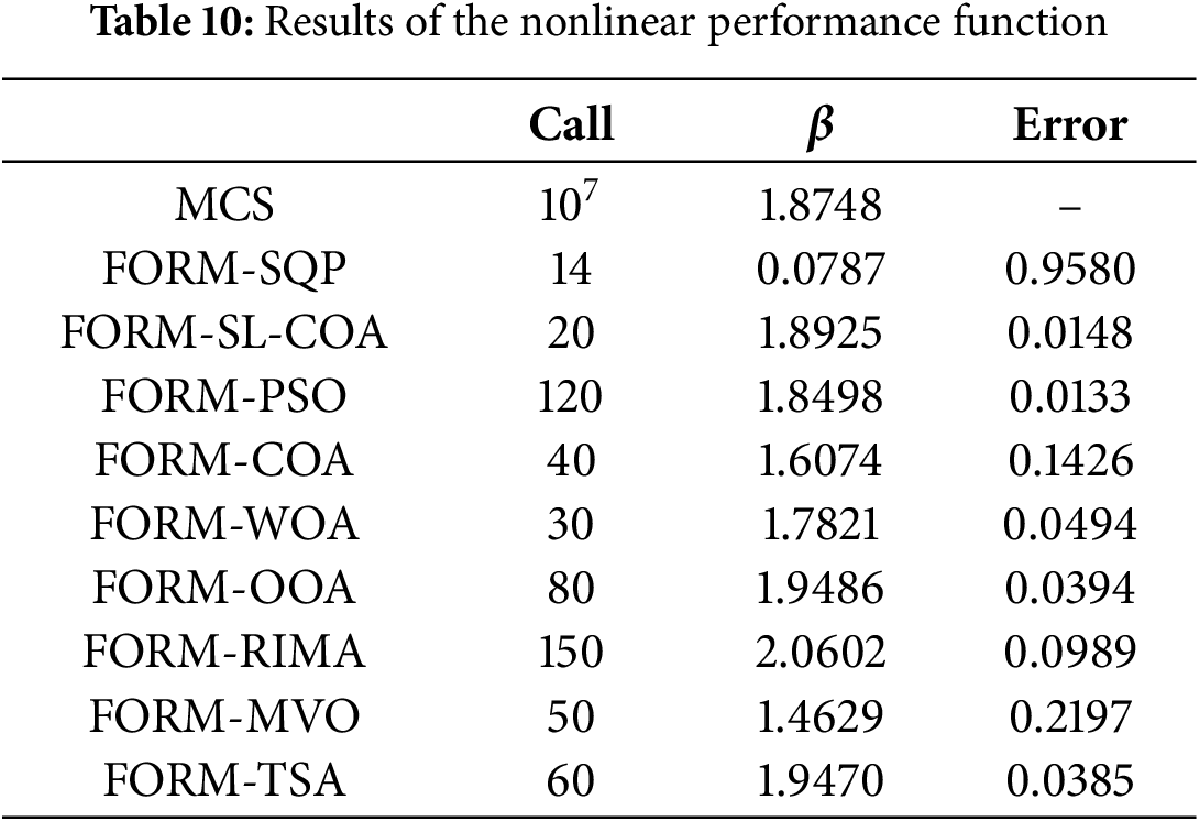
Example 2. Nonlinear performance function

Example 2 presents reliability analysis problems with nonlinear performance functions. Nonlinear performance functions are common in practical engineering structures, such as those resulting from material nonlinearity or geometric nonlinearity in structural responses. Example 2 proves the effectiveness and accuracy of the SL-COA algorithm in handling nonlinear reliability analysis problems, which is crucial for evaluating the safety of complex engineering structures. A nonlinear problem is solved in this example. The LSF is

(35)

where and are normally distributed variables with and . The interval variable . The results are shown in Table 10.

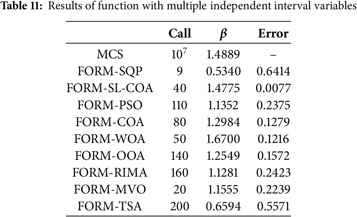
Example 3. Performance function with multiple independent interval variable

Example 3 showcases performance functions with multiple independent interval variables. In practical engineering, certain parameters (such as geometric dimensions, material properties, etc.) may have uncertainties, which are often represented in the form of interval variables. For the third example, an LSF with two interval variables is used to test the proposed framework. The performance function is

(36)

where and are normally distributed variables with and , . The results are shown in Table 11.

Example 4. Performance function with various probability distribution

Example 4 presents performance functions with different probability distributions (such as Weibull, Gumbel, Exponential, and Normal distributions). In practical engineering, the probability of distributions of different parameters may vary, adding complexity to the reliability analysis. A performance function with both normal and non-normal random variables is considered as below.

(37)

The means, standard derivations, and non-normal random variables are considered as shown in Table 12.

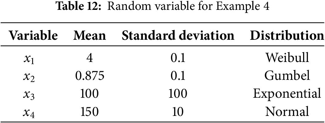
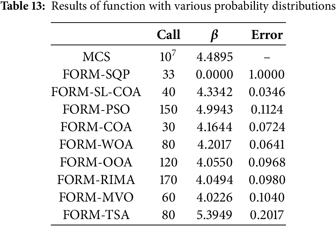
The results are shown in Table 13.

The convergence curve of Example 2, Example 3, and Example 4 is shown in Fig. 15.

Figure 15: Convergence curve of Examples 2, 3, and 4

From the calculation results of the above mathematical examples, it can be seen that SL-COA performs well. Firstly, when the gradient-based FORM cannot obtain acceptable solution results, the FORM based on a heuristic algorithm can obtain effective analysis results. Secondly, compared with other optimization algorithms, the reliability index obtained by SL-COA is closer to the reference result calculated by MCS. This reflects the computational performance of SL-COA, that is, the algorithm can find more acceptable MPP points.

Since the SL-COA-based FORM framework meets the end iteration condition defined in this paper with very few function calls. The reliability index value with more function calls is worth exploring. Therefore, extra testing is conducted by setting a fixed function call number. The results are shown in Table 14.

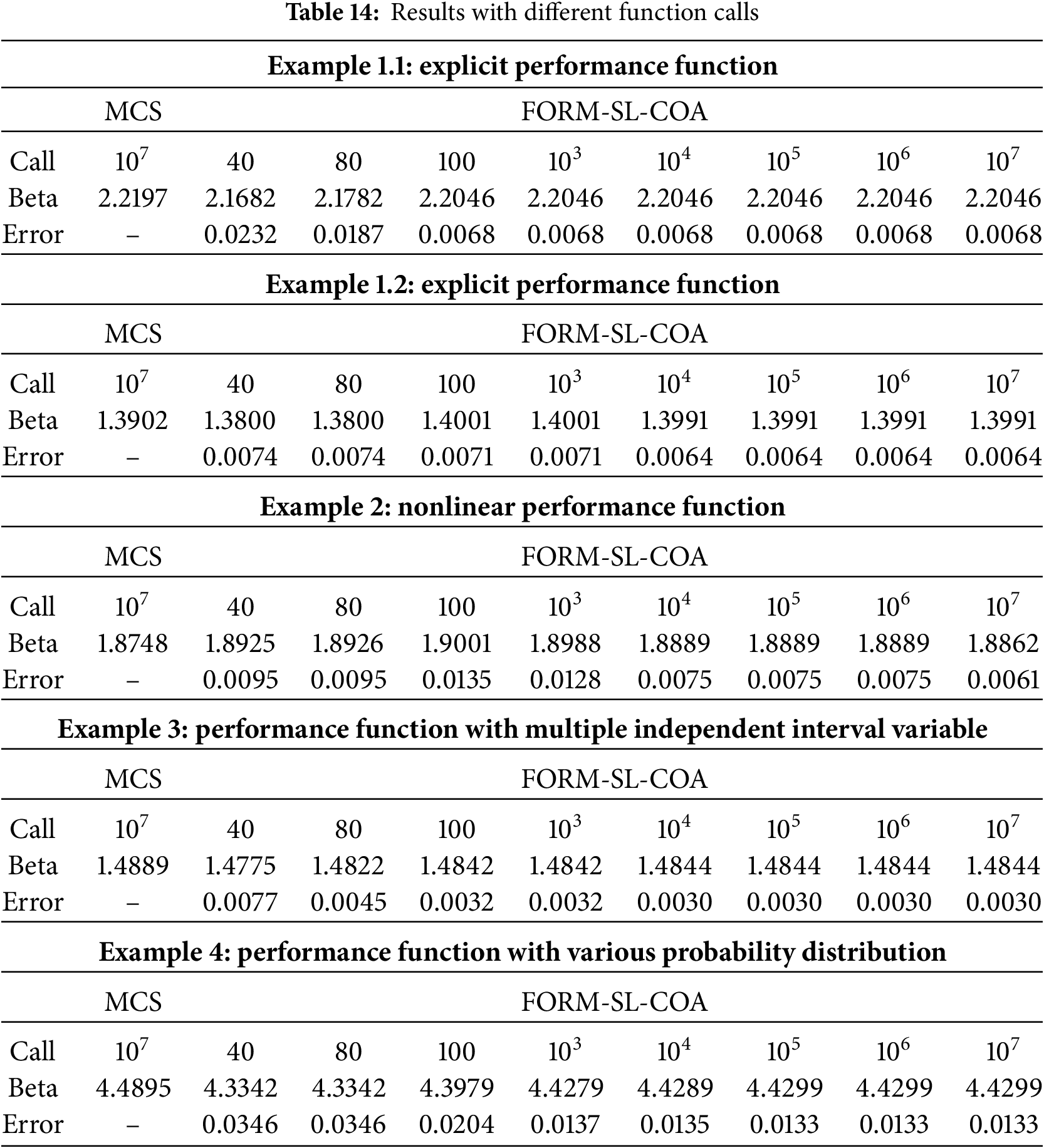
The range of function call values employed in this testing spans from 40 to . This range encompasses the minimum requirement necessary to meet the convergence conditions and extends to the maximum value required by the MCS comparison algorithm. The results demonstrate that the suggested framework can attain greater accuracy with an increased number of function calls, thereby suggesting that the specific interaction values can be adjusted to meet the accuracy requirements in practical engineering applications.

4.3.2 Engineering Examples

In this section, two structural reliability analysis cases are conducted to evaluate the performance of the proposed framework.

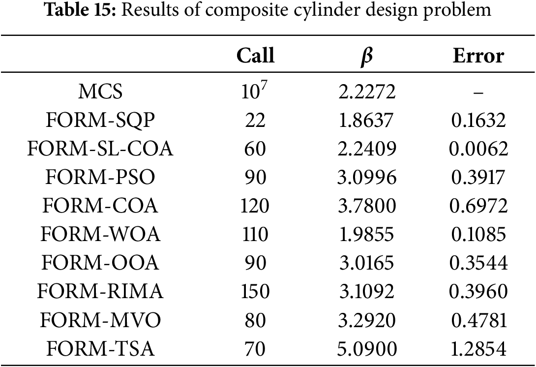
Example 1: Composite cylinder analysis problem

In this example, a composite cylinder case [61] is analyzed. The composite cylinder consists of an inner cylinder and an outer cylinder (shown in Fig. 16). The inner cylinder has an inner diameter of , and an outer diameter of , while the outer cylinder has an inner diameter of and an outer diameter of . The variable is an interval variable. The cylinder is subjected to various loading conditions, and the reliability analysis aims to assess the cylinder’s ability to withstand these loads without failing. The results of composite cylinder design problem are shown in Table 15.

Figure 16: Composite cylinder analysis

Consider:

Subject to:

Parameter:

(38)

where

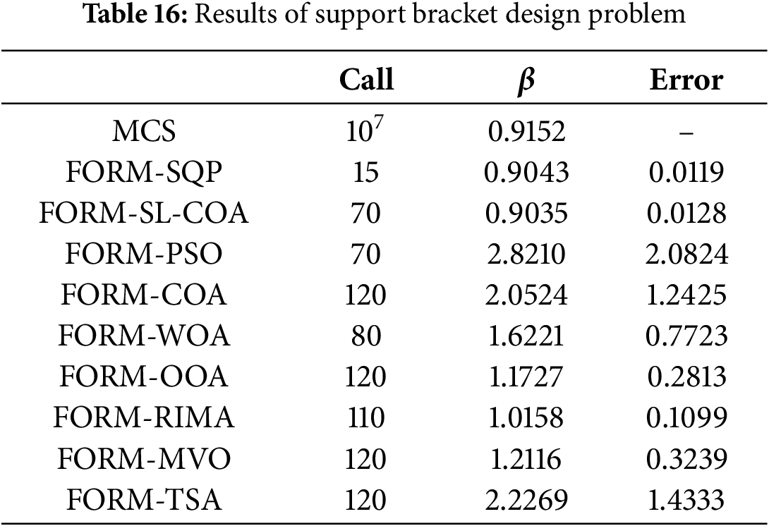
Example 2: Support bracket analysis problem

In this case, a support bracket within an aircraft braking structure is analyzed (the green triangular prism shown in Fig. 17). The material used for this structure is structural steel, and the presence of the triangular ribs in the middle enhances the structural strength. The bracket is subjected to forces generated during braking, and the reliability analysis aims to assess its ability to withstand these forces without failing. Using finite element simulation analysis, the results are obtained and fitted in MATLAB to obtain the LSF. The analysis based on one of the functions is performed below. The results of support bracket are shown in Table 16.

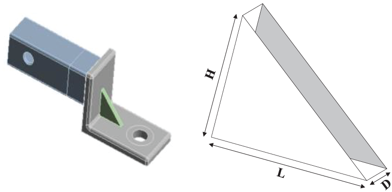
Figure 17: Support bracket analysis

Consider:

Subject to:

Parameter:

(39)

The proposed method successfully solves the engineering problems by delivering acceptable results with minimal function calls in each example. The error in β determined by the proposed methods, when compared to the results obtained through MCS, is approximately 1%. The convergence cure is shown in Fig. 18. The SQP-based FORM exhibits superior performance in these two engineering examples. Although it fails to solve the problems in Section 4.2.1, the results in this section might serve as a reminder that the SQP-based analysis framework is not entirely impractical for addressing hybrid reliability analysis problems. Overall, this result proves the capability of the SL-COA base FORM framework to tackle real engineering problems successfully.

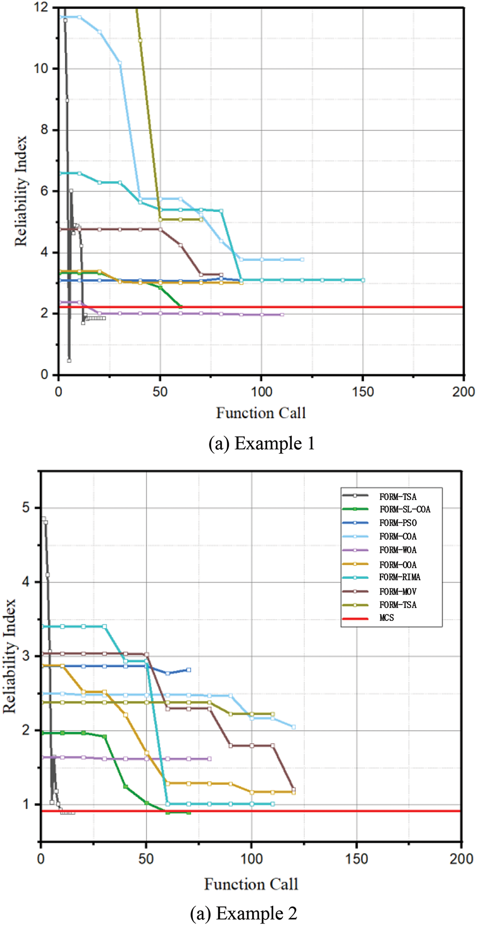
Figure 18: Convergence curve of two engineering problems

5  Conclusions

As a typical analytical strategy for reliability analysis, FORM faces many challenges. In the face of solving complex engineering problems with MCS or improved MCS strategies, FORM may be able to use its low computational difficulty to provide an acceptable analysis result. The main purpose of FORM is to find the exact location of the MPP point. However, there are the following problems: 1) In the past, FORM based on gradients may not be able to obtain convergent results for some reliability analysis problems; 2) Although the FORM using the heuristic algorithm can often obtain convergent reliability analysis results, it may not be able to obtain the acceptable MPP position because the heuristic algorithm is trapped in local optimization. To this end, this study proposes an improved COA optimization algorithm (SL-COA), which is committed to improving the accuracy and robustness of the optimization results. By introducing the SL-COA algorithm into FORM, the effectiveness and practicability of FORM in complex structural reliability analysis are improved.

The main work of this study includes: A new optimization algorithm SL-COA is obtained by improving the COA algorithm through a social learning strategy, which improves its efficiency and robustness in solving medium-dimensional complex problems. The improved effect of the SL-COA algorithm is tested by CEC2005 and CEC2017 test function sets and four engineering examples, which reflect the effectiveness and competitiveness of the algorithm. The performance of FORM based on SL-COA is tested in four mathematical examples and two engineering examples, which shows the effectiveness and practicability of SL-COA in the field of reliability analysis.

New analytical strategies that require lower computational costs and are suitable for multiple reliability problems are also a research direction in future research. In the development of automotive components and systems, reliability and safety are key concerns. SL-COA can be applied to optimize the design of automotive parts, such as engines, transmissions, and body structures, to improve their reliability and durability.

Acknowledgement: We would like to express our sincere gratitude to Beijing Research Institute of Mechanical & Electrical Technology for providing us with the essential venue support for conducting our experiments. The generosity and assistance have been instrumental in the successful completion of this research.

Funding Statement: This research was funded by the National Key Research and Development Program (Grant No. 2022YFB3706904).

Author Contributions: Study conception and design: Yunhan Ling, Huajun Peng, Yiqing Shi, Hui Ma; data collection: Yunhan Ling, Huajun Peng, Yiqing Shi, Chao Xu, Jingzhen Yan; analysis and interpretation of results: Yunhan Ling, Huajun Peng, Hui Ma; draft manuscript preparation: Yunhan Ling, Huajun Peng, Jingjing Wang. All authors reviewed the results and approved the final version of the manuscript.

Availability of Data and Materials: The data will be made available by the corresponding author upon reasonable request.

Ethics Approval: Not applicable.

Conflicts of Interest: The authors declare no conflicts of interest to report regarding the present study.

References

1. Liu X, Li T, Zhou Z, Hu L. An efficient multi-objective reliability-based design optimization method for structure based on probability and interval hybrid model. Comput Methods Appl Mech Eng. 2022;392:114682. doi:10.1016/j.cma.2022.114682. [Google Scholar] [CrossRef]

2. Wang X, Zhao W, Chen Y, Li X. A first order reliability method based on hybrid conjugate approach with adaptive Barzilai-Borwein steps. Comput Methods Appl Mech Eng. 2022;401:115670. doi:10.1016/j.cma.2022.115670. [Google Scholar] [CrossRef]

3. Wang Z, Xiao F, Cao Z. Uncertainty measurements for Pythagorean fuzzy set and their applications in multiple-criteria decision making. Soft Comput. 2022;26:9937–52. doi:10.1007/s00500-022-07361-9. [Google Scholar] [CrossRef]

4. Li XQ, Song LK, Bai GC. Recent advances in reliability analysis of aeroengine rotor system: a review. Int J Struct Integr. 2022;13(1):1–29. doi:10.1108/IJSI-10-2021-0111. [Google Scholar] [CrossRef]

5. Ou Y, Cai Y, Zeng L, Zhao W, Chen Y. A teaching-learning-based optimization algorithm for reliability analysis with an adaptive penalty coefficient. Structures. 2024;65:106695. doi:10.1016/j.istruc.2024.106695. [Google Scholar] [CrossRef]

6. Hao S. I-35W bridge collapse. J Bridge Eng. 2010;15(5):608–14. doi:10.1061/(ASCE)BE.1943-5592.0000090. [Google Scholar] [CrossRef]

7. Li W, Li C, Gao L, Xiao M. Risk-based design optimization under hybrid uncertainties. Eng Comput. 2022;38:1–13. doi:10.1007/s00366-020-01196-4. [Google Scholar] [CrossRef]

8. Li W, Xiao M, Garg A, Gao L. A new approach to solve uncertain multidisciplinary design optimization based on conditional value at risk. IEEE Trans Autom Sci Eng. 2020;18:356–68. doi:10.1109/TASE.2020.2999380. [Google Scholar] [CrossRef]

9. Yang M, Zhang D, Han X. New efficient and robust method for structural reliability analysis and its application in reliability-based design optimization. Comput Methods Appl Mech Eng. 2020;366:113018. doi:10.1016/j.cma.2020.113018. [Google Scholar] [CrossRef]

10. Meng Z, Pang Y, Pu Y, Wang X. New hybrid reliability-based topology optimization method combining fuzzy and probabilistic models for handling epistemic and aleatory uncertainties. Comput Methods Appl Mech Eng. 2020;363:112886. doi:10.1016/j.cma.2020.112886. [Google Scholar] [CrossRef]

11. Meng D, Yang S, Yang H, De JAM, Correia J, Zhu SP. Intelligent-inspired framework for fatigue reliability evaluation of offshore wind turbine support structures under hybrid uncertainty. Ocean Eng. 2024;307:118213. doi:10.1016/j.oceaneng.2024.118213. [Google Scholar] [CrossRef]

12. Zhu SP, Keshtegar B, Bagheri M, Hao P, Trung NT. Novel hybrid robust method for uncertain reliability analysis using finite conjugate map. Comput Methods Appl Mech Eng. 2020;371:113309. doi:10.1016/j.cma.2020.113309. [Google Scholar] [CrossRef]

13. Yang S, Meng D, Yang H, Luo C, Su X. Enhanced soft Monte Carlo simulation coupled with SVR for structural reliability analysis. In: Proceedings of the Institution of Civil Engineers-Transport; Emerald Publishing Limited; 2024. p. 1–41. [Google Scholar]

14. Liu X, Gong M, Zhou Z, Xie J, Wu W. An improved first order approximate reliability analysis method for uncertain structures based on evidence theory. Mech Based Des Struct Mach. 2023;51:4137–54. doi:10.1080/15397734.2021.1956324. [Google Scholar] [CrossRef]

15. Hu Z, Mansour R, Olsson M, Du X. Second-order reliability methods: a review and comparative study. Struct Multidiscipl Optim. 2021;64:1–31. doi:10.1007/s00158-021-03013-y. [Google Scholar] [CrossRef]

16. Yang Z, Ching J. A novel reliability-based design method based on quantile-based first-order second-moment. Appl Math Model. 2020;88:461–73. doi:10.1016/j.apm.2020.06.038. [Google Scholar] [CrossRef]

17. Meng Z, Pang Y, Wu Z, Ren S, Yildiz AR. A novel maximum volume sampling model for reliability analysis. Appl Math Model. 2022;102:797–810. doi:10.1016/j.apm.2021.10.025. [Google Scholar] [CrossRef]

18. Li XQ, Song LK, Bai GC, Li DG. Physics-informed distributed modeling for CCF reliability evaluation of aeroengine rotor systems. Int J Fatigue. 2023;167:107342. doi:10.1016/j.ijfatigue.2022.107342. [Google Scholar] [CrossRef]

19. Abdollahi A, Moghaddam MA, Monfared SAH, Rashki M, Li Y. A refined subset simulation for the reliability analysis using the subset control variate. Struct Saf. 2020;87:102002. doi:10.1016/j.strusafe.2020.102002. [Google Scholar] [CrossRef]

20. Tabandeh A, Jia G, Gardoni P. A review and assessment of importance sampling methods for reliability analysis. Struct Saf. 2022;97:102216. doi:10.1016/j.strusafe.2022.102216. [Google Scholar] [CrossRef]

21. Papaioannou I, Straub D. Combination line sampling for structural reliability analysis. Struct Saf. 2021;88:102025. doi:10.1016/j.strusafe.2020.102025. [Google Scholar] [CrossRef]

22. Meng D, Yang S, de Jesus AMP, Zhu SP. A novel Kriging-model-assisted reliability-based multidisciplinary design optimization strategy and its application in the offshore wind turbine tower. Renew Energy. 2023;203:407–20. doi:10.1016/j.renene.2022.12.062. [Google Scholar] [CrossRef]

23. Meng D, Yang S, De JAM, Fazeres-Ferradosa T, Zhu SP. A novel hybrid adaptive Kriging and water cycle algorithm for reliability-based design and optimization strategy: application in offshore wind turbine monopile. Comput Methods Appl Mech Eng. 2023;412:116083. doi:10.1016/j.cma.2023.116083. [Google Scholar] [CrossRef]

24. Ling Y, Shi Y, Hou H, Pan L, Chen H, Liang P, et al. Enhanced dung beetle optimizer for Kriging-assisted time-varying reliability analysis. AIMS Math. 2024;9(10):29296–332. doi:10.3934/math.20241420. [Google Scholar] [CrossRef]

25. Zhou Y, Lu Z, Yun W. Active sparse polynomial chaos expansion for system reliability analysis. Reliability Eng Syst Saf. 2020;202:107025. doi:10.1016/j.ress.2020.107025. [Google Scholar] [CrossRef]

26. Meng D, Li Y, He C, Guo J, Lv Z, Wu P. Multidisciplinary design for structural integrity using a collaborative optimization method based on adaptive surrogate modelling. Mater Design. 2021;206:109789. doi:10.1016/j.matdes.2021.109789. [Google Scholar] [CrossRef]

27. Afshari SS, Enayatollahi F, Xu X, Liang X. Machine learning-based methods in structural reliability analysis: a review. Reliability Eng Syst Saf. 2022;219:108223. doi:10.1016/j.ress.2021.108223. [Google Scholar] [CrossRef]

28. Luo C, Keshtegar B, Zhu SP, Niu X. EMCS-SVR: hybrid efficient and accurate enhanced simulation approach coupled with adaptive SVR for structural reliability analysis. Comput Methods Appl Mech Eng. 2022;400:115499. doi:10.1016/j.cma.2022.115499. [Google Scholar] [CrossRef]

29. Keshtegar B, Seghier MEAB, Zio E, Correia JA, Zhu SP, Trung N-T. Novel efficient method for structural reliability analysis using hybrid nonlinear conjugate map-based support vector regression. Comput Methods Appl Mech Eng. 2021;381:113818. doi:10.1016/j.cma.2021.113818. [Google Scholar] [CrossRef]

30. Meng D, Yang H, Yang S, Zhang Y, De Jesus AM, Correia J, et al. Kriging-assisted hybrid reliability design and optimization of offshore wind turbine support structure based on a portfolio allocation strategy. Ocean Eng. 2024;295:116842. doi:10.1016/j.oceaneng.2024.116842. [Google Scholar] [CrossRef]

31. Xue Y, Deng Y. Extending set measures to orthopair fuzzy sets. Fuzziness Knowl-Based Syst. 2022;30:63–91. doi:10.1142/S0218488522500040. [Google Scholar] [CrossRef]

32. Yang S, Meng D, Wang H, Chen Z, Xu B. A comparative study for adaptive surrogate-model-based reliability evaluation method of automobile components. Int J Struct Integr. 2023;14:498–519. doi:10.1108/IJSI-03-2023-0020. [Google Scholar] [CrossRef]

33. Yang S, Meng D, Wang H, Yang C. A novel learning function for adaptive surrogate-model-based reliability evaluation. Philos Trans R Soc A. 2024;382(2264):20220395. doi:10.1098/rsta.2022.0395. [Google Scholar] [PubMed] [CrossRef]

34. Yang S, Meng D, Guo Y, Nie P, Jesus AMDE. A reliability-based design and optimization strategy using a novel MPP searching method for maritime engineering structures. Int J Struct Integr. 2023;14:809–26. doi:10.1108/IJSI-06-2023-0049. [Google Scholar] [CrossRef]

35. Zhu SP, Keshtegar B, Chakraborty S, Trung NT. Novel probabilistic model for searching most probable point in structural reliability analysis. Comput Methods Appl Mech Eng. 2020;366:113027. doi:10.1016/j.cma.2020.113027. [Google Scholar] [CrossRef]

36. Zhang D, Zhang J, Yang M, Wang R, Wu Z. An enhanced finite step length method for structural reliability analysis and reliability-based design optimization. Struct Multidiscipl Optim. 2022;65:231. doi:10.1007/s00158-022-03294-x. [Google Scholar] [CrossRef]

37. Yang M, Zhang D, Wang F, Han X. Efficient local adaptive Kriging approximation method with single-loop strategy for reliability-based design optimization. Comput Methods Appl Mech Eng. 2022;390:114462. doi:10.1016/j.cma.2021.114462. [Google Scholar] [CrossRef]

38. Keshtegar B, Zhu SP. Three-term conjugate approach for structural reliability analysis. Appl Math Model. 2019;76:428–42. doi:10.1016/j.apm.2019.06.022. [Google Scholar] [CrossRef]

39. Roudak MA, Karamloo M. Establishment of non-negative constraint method as a robust and efficient first-order reliability method. Appl Math Model. 2019;68:281–305. doi:10.1016/j.apm.2018.11.021. [Google Scholar] [CrossRef]

40. Zhu SP, Keshtegar B, Seghier MEAB, Zio E, Taylan O. Hybrid and enhanced PSO: novel first order reliability method-based hybrid intelligent approaches. Comput Methods Appl Mech Eng. 2022;393:114730. doi:10.1016/j.cma.2022.114730. [Google Scholar] [CrossRef]

41. Yang S, Guo C, Meng D, Guo Y, Guo Y, Pan L, et al. MECSBO: multi-strategy enhanced circulatory system based optimisation algorithm for global optimisation and reliability-based design optimisation problems. Collab Intell Manuf. 2024;6(2):e12097. doi:10.1049/cim2.12097. [Google Scholar] [CrossRef]

42. Kokash N. An introduction to heuristic algorithms. Dep Inform Telecommun. 2005:1–8. [Google Scholar]

43. Vinod Chandra SS, Harshil Anand A. Nature inspired meta heuristic algorithms for optimization problems. Computing. 2022;104(2):251–69. doi:10.1007/s00607-021-00955-5. [Google Scholar] [CrossRef]

44. Pedroso DM. FORM reliability analysis using a parallel evolutionary algorithm. Struct Saf. 2017;65:84–99. doi:10.1016/j.strusafe.2017.01.001. [Google Scholar] [CrossRef]

45. Zhong C, Wang M, Dang C, Ke W, Guo S. First-order reliability method based on Harris Hawks Optimization for high-dimensional reliability analysis. Struct Multidiscipl Optim. 2020;62(4):1951–68. doi:10.1007/s00158-020-02587-3. [Google Scholar] [CrossRef]

46. Dehghani M, Montazeri Z, Trojovská E, Trojovský P. Coati optimization algorithm: a new bio-inspired metaheuristic algorithm for solving optimization problems. Knowl Based Syst. 2023;259:110011. doi:10.1016/j.knosys.2022.110011. [Google Scholar] [CrossRef]

47. Ioffe S. Batch normalization: accelerating deep network training by reducing internal covariate shift. arXiv:1502.03167. 2015. [Google Scholar]

48. Kennedy J, Eberhart R. Particle swarm optimization. In: Proceedings of ICNN’95—International Conference on Neural Networks; 1995; Perth, WA, Australia: IEEE. Vol. 4, p. 1942–8. doi:10.1109/ICNN.1995.488968. [Google Scholar] [CrossRef]

49. De OMAM, Stutzle T, Van den EK, Dorigo M. Incremental social learning in particle swarms. IEEE Trans Syst Man Cybern Part B (Cybern). 2010;41:368–84. [Google Scholar]

50. Lu P, Wen F, Li Y, Chen D. Individual behaviors, social learning, and swarm intelligence: real case and counterfactuals. Expert Syst Appl. 2022;207:117878. doi:10.1016/j.eswa.2022.117878. [Google Scholar] [CrossRef]

51. Shafiq M, Ali ZA, Israr A, Alkhammash EH, Hadjouni M. A multi-colony social learning approach for the self-organization of a swarm of UAVs. Drones. 2022;6:104. doi:10.3390/drones6050104. [Google Scholar] [CrossRef]

52. Mirjalili S, Lewis A. The whale optimization algorithm. Adv Eng Softw. 2016;95:51–67. doi:10.1016/j.advengsoft.2016.01.008. [Google Scholar] [CrossRef]

53. Dehghani M, Trojovský P. Osprey optimization algorithm: a new bio-inspired metaheuristic algorithm for solving engineering optimization problems. Front Mech Eng. 2023;8:1126450. doi:10.3389/fmech.2022.1126450. [Google Scholar] [CrossRef]

54. Su H, Zhao D, Heidari AA, Liu L, Zhang X, Mafarja M. RIME: a physics-based optimization. Neurocomputing. 2023;532:183–214. doi:10.1016/j.neucom.2023.02.010. [Google Scholar] [CrossRef]

55. Mirjalili S, Mirjalili SM, Hatamlou A. Multi-verse optimizer: a nature-inspired algorithm for global optimization. Neural Comput Appl. 2016;27:495–513. doi:10.1007/s00521-015-1870-7. [Google Scholar] [CrossRef]

56. Kiran MS. TSA: tree-seed algorithm for continuous optimization. Expert Syst Appl. 2015;42:6686–98. doi:10.1016/j.eswa.2015.04.055. [Google Scholar] [CrossRef]

57. Kamil AT, Saleh HM, Abd-Alla IH. A multi-swarm structure for particle swarm optimization: solving the welded beam design problem. J Phys: Conf Series. 2021;1804(1):012012. doi:10.1088/1742-6596/1804/1/012012. [Google Scholar] [CrossRef]

58. Tzanetos A, Blondin M. A qualitative systematic review of metaheuristics applied to tension/compression spring design problem: current situation, recommendations, and research direction. Eng Appl Artif Intell. 2023;118:105521. doi:10.1016/j.engappai.2022.105521. [Google Scholar] [CrossRef]

59. Min F, Huang H. An improved dragonfly optimization algorithm for solving numerical and three-bar truss optimization problems. In: 2021 5th Asian Conference on Artificial Intelligence Technology (ACAIT); Haikou, China; 2021. p. 204–18. [Google Scholar]

60. Mohammed H, Rashid T. A novel hybrid GWO with WOA for global numerical optimization and solving pressure vessel design. Neural Comput Appl. 2020;32(18):14701–18. doi:10.1007/s00521-020-04823-9. [Google Scholar] [CrossRef]

61. Gunawan S, Azarm S, Wu J, Boyars A. Quality-assisted multi-objective multidisciplinary genetic algorithms. AIAA J. 2003;41:1752–62. doi:10.2514/2.7293. [Google Scholar] [CrossRef]