Semantic Malware Classification Using Artificial Intelligence Techniques

1  Introduction

Malicious software (malware) is currently considered the main weapon for carrying out malicious actions in cyberspace to breach any organization’s cybersecurity [1]. It is one of the most effective cyberattack vectors today [2], and driven by economic benefits, malware attacks increase significantly daily [3].

Based on statistics published by AV-Atlas in 2024, approximately 1.444 million malware samples were identified between 2008 and 2024. In the last year, new malware specimens have grown by 7.14% [4].

Based on the above, it can be concluded that the threat of malware is growing, which brings the need to develop more effective methods for its detection and classification. The malware affects all operating systems with their different file formats, from Windows [2], Linux [5], IoT devices [6] and others. Research efforts are underway to develop new methods to detect malware effectively and efficiently to defend against these constantly evolving and growing threats [2].

Evasive techniques, such as packaging, encryption, polymorphism, metamorphism, and others, are used by malware producers to quickly change their behavior and formats to avoid detection, thus generating a large amount of new malware as variants of existing malware [7].

As attacks become more sophisticated, research into innovative approaches, such as using Artificial Intelligence (AI) techniques, is warranted to improve the accuracy and speed of classification and detection of this threat by the various anti-malware systems currently in use [8].

The need to develop techniques that generalize well the identification of new malware makes the task of malware detection suitable for machine learning (ML) [9]. The use of ML in malware detection is under constant study, as can be observed in the research articles in [2,10].

Convolutional neural networks (CNNs) are a class of deep learning neural networks designed for multidimensional data processing, which, through convolutions, make it possible to extract features for learning from raw data such as images, spectrograms, signals, and text sequences [11,12]. In addition, these are being applied to malware detection because of their generalization properties in unknown data by using malicious Portable Executable (PE) file features.

Malware in PE format poses a major threat to Windows users due to its widespread adoption and portability. This is mainly due to the worldwide popularity and file portability of the Windows family of operating systems. Probably the main reason is that the file in this format, in addition to including all the data and instructions necessary to execute an attack, can also be easily executed by any user, thus becoming the main target of attackers to maximize the benefits of attacks [2].

Several approaches have been employed to feed deep learning systems for malware detection or classification. Both static and dynamic features can be extracted from PE files, such as header information, contents of strings, sequences of bytes, lists of opcodes, calls to APIs, and others. The use of raw bytes is a viable alternative for identifying malware in PE files [9], but without considering any semantic context [13].

The literature review identified a lack of approaches that effectively combine semantics with deep learning techniques, such as convolutional neural networks, for malware classification. Many previous studies have not comprehensively addressed the interaction between these two fields, which limits detection and classification capabilities in complex scenarios.

This research proposes an innovative approach for malware classification using convolutional neural network (ML) techniques using statically extracted raw byte sequences, considering the semantic context represented by the PE executable file format.

The main contribution of this work is the proposal to apply the concept of semantic variation for the static extraction of malware resources in PE format to feed neural network systems. This is done by separating PE files into parts based on the semantic meanings that bytes can have. The aim is to improve performance and malware classification results using Convolutional Neural Network (CNN) architectures.

In addition, it is evaluated whether the use of data extracted based on semantic location can present better results than the use of the sequence of bytes of the whole file and whether the number of trainable parameters in CNNs can be reduced while maintaining performance rates. In conclusion, this research seeks to provide an innovative approach that combines advanced machine learning techniques with semantic processing to improve the identification of malicious patterns.

The paper is organized as follows: Section 2 presents the concepts and related work, Section 3 describes the objectives, methods, proposals, and metrics used in the research, and Section 4 details the procedures performed to execute the practical tests. Section 5 presents and discusses the results, and finally, Section 6 concludes with insights and future directions.

2  Background and Related Work

Deep learning (DL) focuses on developing algorithms that automatically improve through experience. Positioned at the intersection of computer science and statistics, DL has become central to Artificial Intelligence (AI) and, more recently, data science [14]. It employs multiple layers of information processing in hierarchical supervised architectures to extract relevant features and perform joint discrimination [15]. These layers enable the learning of data representations with various levels of abstraction, enhancing pattern analysis and understanding from unsupervised resources.

The strength of deep networks lies in their ability to discover complex structures in large datasets. Utilizing backpropagation algorithms, these computational models can adjust their internal parameters to compute representations in each layer based on the previous layer’s outputs [11].

The use of DL can be observed in many knowledge domains. These include natural language processing, speech recognition, image recognition, medical applications, semantic segmentation, scene labeling, face recognition, object detection, video object segmentation, background and foreground separation, graph-based applications, intelligent transportation systems, financial modeling, policing, and marketing [14].

Recently, DL models have been applied and adapted for malware classification and detection [2,16], with most datasets comprising PE files. CNN, a type of DL, is designed to process multidimensional data. Many data modalities can be represented as multiple arrays: signals, sequences, and language in one dimension (1D); images (such as a color image composed of three two-dimensional arrays containing the intensity of pixels in three color channels) [12] or audio spectrograms in two dimensions (2D); and videos or volumetric images in three dimensions (3D) [11].

Among the different types of layers in CNNs are convolutional, pooling, and fully connected layers. These layers transform the original input using convolutional and reduction techniques to produce class scores for classification and regression purposes [17].

Fig. 1 shows a typical basic structure of a CNN applied to malware detection, using the three common layers to produce the output as a sample classification probability. The purpose of the convolutional layer is to extract high-level features from the input data and pass them to the next layer in the form of feature maps. Each convolutional operation is specified by a step and the filter size, and it can have a padding option.

Figure 1: Basic CNN architecture applied to malware detection (Source: Vinayakumar et al., 2019 [7])

The pooling layers aim to gradually reduce the dimensionality of the representation, reducing the number of parameters and the computational complexity of the model [17]. This layer receives each feature map output from the convolutional layer and prepares a condensed feature map.

Fully connected layers are typically used in the final stages of a CNN. These layers connect all the inputs of one layer to each activation unit of the next layer, abstracting the low-level information generated in previous layers to a final decision [15].

Malware detection systems examine specific files to determine whether they are malicious. Early antivirus products relied on monitoring machines for specific indicators of compromise, such as file names or exact signatures (specific sequences of bytes or strings from the contents of a file) [16]. ML offered the most promising strategies for detecting malware attacks on enterprise information systems in this context due to its increased accuracy and precision [18].

Three main objectives can be applied to malware analysis using ML. The first is malware detection, and the second is similarity analysis to learn how variants differ from existing ones, including variant detection, family, similarity, and difference; and finally, categorization to learn about the behavior and goals of the malware [10].

Malicious artifact analysis is a complex process focused on detecting whether a binary is malicious or not or classifying it into families or variants of malware [13]. Distinguishing between the categories of malware is important to understanding how they can infect computer systems, the threat level, and the ways to protect against them [19].

Malware detection can be divided into two general categories: anomaly-based and signature-based detection. Both can be further subdivided into three traditional categories of malware analysis: static, dynamic, and hybrid, each with its advantages and limitations [20]. Traditional malware analysis cannot keep up with the rate of new attacks, new variants, and millions of daily attacks. ML presents itself as an alternative [21].

Malware detection using standard signature-based methods is becoming increasingly difficult due to the use of polymorphic, metamorphic, encryption, and compression techniques to evade detection by anti-malware tools or the use of lateral mechanisms to automatically update to a newer version in short periods [22].

Recent research indicates that existing ML and DL techniques can enable superior detection of emerging and novel malware [2] and can be more efficient than traditional signature-based approaches in detecting zero-day threats [23]. ML has the potential to significantly change the cybersecurity landscape by addressing the growing challenges related to malware classification [24] and identifying shared features among samples that cannot be classified using simple rules [16]. DL models can learn arbitrary patterns in streams of bytes and exhibit satisfactory performance in detecting malware [25].

Based on Musser et al. [26], the first studies using machine learning for malware detection were initiated in 1996 by IBM researchers to classify boot sector viruses. Dambra et al. [27] defined limitations in current malware detection and classification approaches, indicating future directions for improving the effectiveness of malware detection models. Hence, it compared static and dynamic features in malware classification using the Random Forest (RF) and XGBoost AI models.

Massun et al. [28] presented a comparative study of several ML or machine learning models for the detection and specific classification of ransomware. They highlighted the effectiveness of the Randon Forest model with 99% classification accuracy. The study concluded that machine learning is a viable strategy for detecting ransomware variants and families, overcoming the limitations of traditional detection systems. Another similar study is the one by Ramon et al. [29] that employed recursive temporal contextualization to identify and classify ransomware activities in real-time by analyzing sequences of system events and the one performed by Wasoye et al. [30] to propose an innovative approach to ransomware classification using the Binary Transformation and Lightweight Signature (BTLS) algorithm for static and dynamic feature extraction from samples combined with machine learning techniques.

Aslan et al. [31] proposed a new malware classification framework based on a hybrid DL approach, which uses a Hybrid Deep Neural Network to extract distinctive features from malware images. The classification method combined two pre-trained models: AlexNet and ResNet-50.

Another innovative approach to malware classification [32] is using CNNs to extract features from malware representations as grayscale images. The study utilized the VGG19 neural network and spatial convolutional attention mechanisms to improve malware detection accuracy.

Chaganti et al. [33] used another innovative approach to malware classification using image representations and EfficientNet convolutional neural networks. Liu et al. [34] presented an automatic malware classification system based on a Spiking neural networks (SNNs) model, combining feature extraction from grayscale images, n-grams of opcodes, and import functions.

Yoo et al. [35] introduced a hybrid malware detection model that combines random forest and DL techniques, achieving a detection rate of 85.1% with a low false positive rate. The main contributions included optimizing voting rules and using hybrid features to improve the classification accuracy of malicious and benign files, thus facilitating fast and effective malware detection.

A comprehensive review of malware classification and composition analysis was conducted by Abusitta et al. in [36]. Problems and challenges in malware detection were identified, and a new taxonomy was proposed to organize existing approaches and provide a framework for improving feature extraction using deep learning techniques.

A comparative table summarizing AI-based malware detection methods is adapted to include shallow learning (SL), deep learning (DL), and bio-inspired techniques, as these are the primary categories discussed in Wolsey’s review [37]. The following is an adapted representation combining key AI techniques and their features, Table 1:

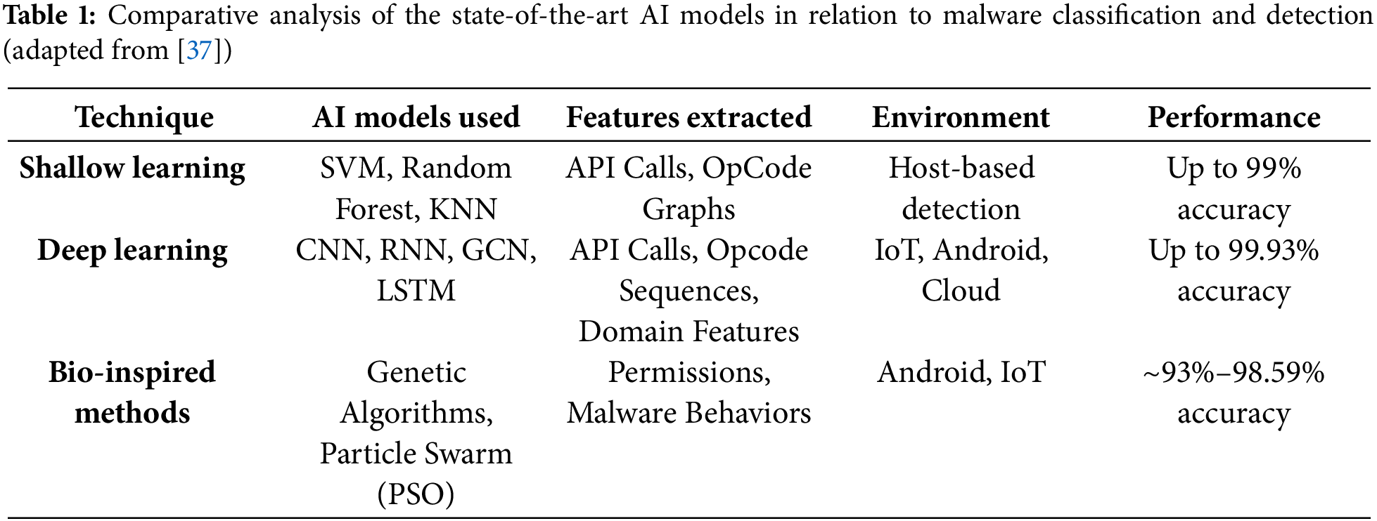
The integration of CNNs into malware detection has proven highly effective, particularly for analyzing PE files. As highlighted by Jiang et al. [38] in the cited review [37], a novel approach using CNNs combined with an evolutionary fuzzy LSTM immune system achieved 98.59% accuracy in PE malware detection. Another research work by Maniriho et al. [39], based on the use of CCN as an AI model, obtained a performance of 99.93% accuracy.

The ability of CNNs to process visualized binary data from malware files and extract hierarchical features makes them superior in analyzing complex data, enabling the extraction of complex features that static or heuristic methods can miss.

Fig. 2 presents an overview of the ML process for malware detection, illustrating three major stages: data acquisition, resource extraction, and training models and making predictions [2].

Figure 2: A general machine learning process for malware detection (Source: Ling et al. 2023 [2])

The first step involves structuring a database with samples, considering analysis objectives, the execution platform, the number of samples, the availability of binaries, and available labels [13]. Evaluating the effectiveness of classic DL architecture requires creating a large dataset with various samples. Publicly available datasets for potential malware detection research are limited due to the privacy preservation policies of individuals and organizations [7].

The objective of the second step is to extract intrinsic properties from the PE files to feed learning models for malware detection and perform necessary preprocessing, such as transforming the properties into appropriate numerical resources [2], to ensure the effectiveness and applicability of ML [40]. Different categories of features extracted from PE files, both static and dynamic, can be utilized to generate resources for learning systems [10,21].

Coull et al. [41] indicated that deep learning architectures with raw byte data inputs are a viable alternative to traditional machine learning for malware classification, eliminating the costs of manual identification work for resource identification.

Raff et al. [9] demonstrated that neural networks can extract the underlying high-level interpretation of raw bytes, making it possible to develop malware detectors without manual feature extraction. They used a feature vector extracted statically from the entire binary.

In the third step, the resources are utilized to train neural networks, evaluate them, and predict unknown data. The model can also be utilized to produce classification results with broader outputs, such as similarity or categorization analysis.

The use of raw byte sequences as a resource for malware detection was proposed by [4], apparently the first of its kind to use a sequence containing the entire file. CNNs can extract the underlying high-level interpretations of raw bytes, making it possible to develop malware detectors without manually extracting features [25].

This capability highlights CNN’s role in bridging the gap between high detection and classification accuracy, better performance in identifying complex patterns, and adaptability to evolving malware. This is the main reason that justifies the choice of this AI model in the present research.

Malware in PE format remains the predominant threat to both personal and corporate users. This is mainly due to the worldwide popularity of the Windows family of operating systems. The portability of PE files between operating system families also contributed. Probably the main reason is that the file in this format, in addition to including all the data and instructions needed to execute an attack, can also be easily executed by any user, thus becoming the main target for attackers to maximize the benefit of attacks [2].

It can be considered a sequence of bytes to apply static analysis and detection techniques to a malware sample in PE format, which is a binary file. The sequence represents the file’s structure, control information, codes, and data. There can be different semantic contexts for each set of information.

Developing detection rules that capture the semantics of a malicious sample can be more challenging to circumvent because malware developers can apply complex modifications to avoid detection [10]. Semantic variation is a concept that occurs when malware is represented as a sequence of bytes without considering the different types of information existing in a PE file [13].

The bytes of a PE file can contain various types of information that can exhibit spatial correlation, depending on the section in which they are stored [9]. In addition, binaries can have varying lengths, as they are sequences of bytes. Demetrio et al. [42] emphasized that no definitive metrics can be applied to these bytes, as each value represents either an instruction or data, making it challenging to establish a standardized approach.

The concept of semantic variation is illustrated in Fig. 3, where the author presents an example in which the byte 64h has different meanings depending on its location in the PE file. Based on this foundation, this work proposes applying the concept of semantic variation to segregate byte extraction from PE files. Then, each segregated set of bytes will feed a specific CNN.

Figure 3: Semantic variation example: (a) Section .text malware code; (b) data section malware data; (c) Malware header data

As a conclusion to this section and as mentioned in the “Introduction” section, the main gap identified in the literature review is the lack of approaches that effectively combine semantics with deep learning techniques, such as convolutional neural networks, for malware classification. Many previous studies have not comprehensively addressed the interaction between these two fields, which limits detection and classification capabilities in complex scenarios.

Based on the literature review conducted, the main contribution of the present research related to malware classification is the use of the semantic approach in extracting data from a PE file of a malware specimen. This allows a more accurate classification of malware by considering the structure and meaning of the bytes rather than simply their full byte sequence and can be a breakthrough for malware detection systems.

In addition, the use of CNN architecture adapted to work with semantically extracted data can lead to an advance in the application of AI techniques in the field of cybersecurity and a reduction of trainable parameters by using a smaller volume of semantically extracted data. This can lead to more efficient models without sacrificing performance. Finally, algorithms for data preparation, feature extraction, and dataset separation are developed, providing practical tools for malware detection and classification research.

3  Materials and Methods

3.1 Objectives

The main contribution of this study is to verify how using raw bytes extracted from different parts of PE files (semantic parts) can impact performance and malware classification results using CNN architectures through applied research. Hence, the following objectives are defined:

1.   Conducting bibliographic research on the state of the art in the use of CNN to detect and classify malware in PE format.

2.   Preparing a dataset of malware samples to conduct the applied research tests.

3.   Analyzing and separating PE files into parts based on the semantic meanings of the bytes, considering the headers, codes, and data.

4.   Analyzing and adapting CNN architectures for training, validation tests, prediction, and metrics collection.

5.   Analyzing the results obtained in the training and verifying if they can be compared to related research results.

During the research, the following hypotheses related to the application of the semantic approach are assessed:

1.   The use of data extracted based on the semantic location of sample files can show better results than utilizing a sequence of bytes from the whole file.

2.   The number of trainable parameters in CNN can be reduced using a smaller volume of data extracted based on semantic meaning while maintaining performance rates.

3.   Models from CNN architectures can be reused for training and testing with semantic part data.

4.   CNN models trained in semantic feature analysis can accurately detect unknown samples.

A four-phase approach is adopted to achieve the objectives of the study, as represented in Fig. 4. The first phase involves preparing the database for research. The initial data used consists of samples of executable files in PE format labeled in malware families. This study analyzes the dataset and applies techniques to correct distortions.

Figure 4: Summary of the investigation process method

The second phase includes activities to apply the semantic concept in extracting data from executable files in PE format to generate intermediate data to feed the CNN input layers.

The third phase involves selecting, preparing, and using the CNN model with the semantic resources extracted in the previous step. A model known in the research environment for malware classification was chosen to fulfill the research objectives and provide a basis for comparing the results.

The fourth phase is to analyze the collected data and compare the results obtained in the tests with the four categories of semantic resources extracted from the malware samples to assess whether the semantic separation achieved the expected results. Then, the results were compared to those of similar research using raw byte data or the same metrics.

3.2 Semantic Propose

Windows executables must adhere to the PE specification, a file format used for executables, object code, DLLs, and other file types (.cpl, .exe, .dll, .ocx, .sys, .scr, .drv) across both 32-bit and 64-bit Windows operating systems. Malware, such as any legitimate executable, must comply with this specification to be recognized and executed by the operating system, even though it can manipulate the structure by mixing or scrambling PE sections or embedding code within data sections while preserving the overall compatibility with the PE format.

The semantic proposal of this work is depicted in Fig. 5, providing a comprehensive visualization of the structure and organization of a PE file. The first part of the figure presents a high-level structure of a PE file, highlighting its main components: the header and sections. The header is responsible for storing essential information about the file, such as addresses and sizes, while the sections are organized based on their functionalities, such as executable code, data, and debugging information. This structural view facilitates the understanding of the internal organization of a PE file, providing a foundation for further analysis.

Figure 5: Representation of the semantic proposal: (a) PE file structure; (b) Semantic parts

The second part of the figure illustrates how the semantic parts were defined and organized in this research work. These semantic parts were created by grouping sections based on their specific purposes: header, code (.text and .debug), data (.data, .idata, and .rdata), and an integrated file view (file), which consolidates information from all previous groups to provide a comprehensive perspective of the PE file. This semantic organization enables effective extraction and structuring of data, optimizing its use in deep learning models such as convolutional neural networks (CNNs). Section 4.2 specifies the criteria utilized to separate the semantic parts.

Finally, the proposed model in this research was conceived based on a dataset containing whole malware files, which happened to be in the PE format for the Windows system. However, considering that the PE and Executable and Linkable Format (ELF) of Linux or UNIX systems that have reasonably similar structures (Fig. 6 [43]), it will only need to rewrite the function that retrieves the raw bytes from the file and classifies them into semantic parts to utilize a dataset of ELF malware. The LIEF library, utilized to analyze and extract bytes, supports both formats. Future work can consist of extending this model for malware classification and detection on Linux systems with ELF file format.

Figure 6: Comparison of PE and ELF file formats: (a) Windows PE format; (b) Linux EL format (Source: Wang et al. 2021 [43])

3.3 Method Followed in the Research

A cross-validation method adapted from the k-fold cross-validation proposal is used [44] to collect consistent data during practical tests with neural network models using semantic parts data and to allow better validation of the results. The method, called incremental cross-validation, consists of two techniques applied before each test performance. Based on the algorithms proposed in the first group of procedures, the first technique aims to separate the dataset into three data sets, with 80% for training, 10% for validation, and 10% for testing and prediction, randomly selected. A high-level representation of how the datasets are distributed, as shown in Fig. 7.

Figure 7: k-fold cross-validation representation

The second technique in Fig. 8 represents how the size of semantic input data increases in successive training rounds. The model learns in a controlled and gradual manner by starting with smaller data segments (input bytes) and progressively expanding them by adding incremental portions (increment). This approach raises smoother optimization and reduces the risks of overfitting or underfitting as the model is exposed to increasingly larger and more complex data representations.

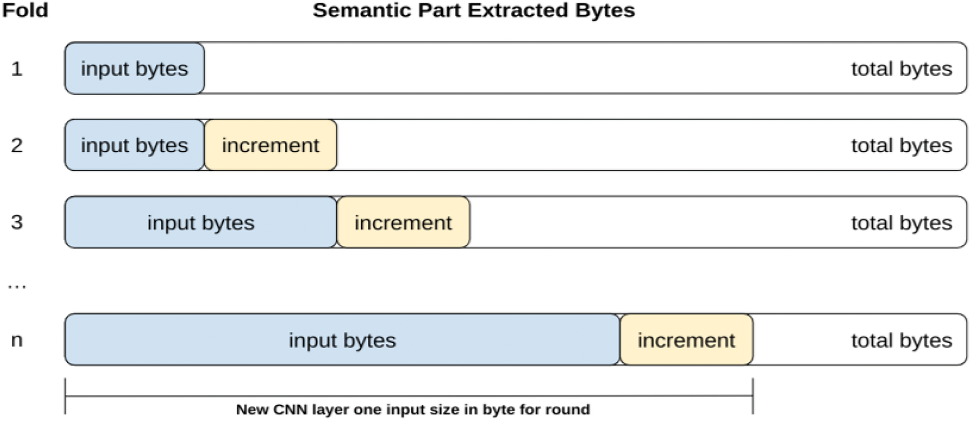
Figure 8: Incremental data representation

Each fold (Fold 1, Fold 2, and others) corresponds to a training round, where the input data size increases by a predefined value (increment). The last fold (n) cannot include the entire dataset (raw bytes of the malware’s semantic parts) if the number of rounds is insufficient to ensure that the model is trained on the full scope of data for a semantic part.

It defines the amount of data in bytes of the semantic parts utilized to feed the CNN input layer within a defined limit. The amount (n) was changed incrementally between tests, with the primary objective of directly assessing the impact on the results.

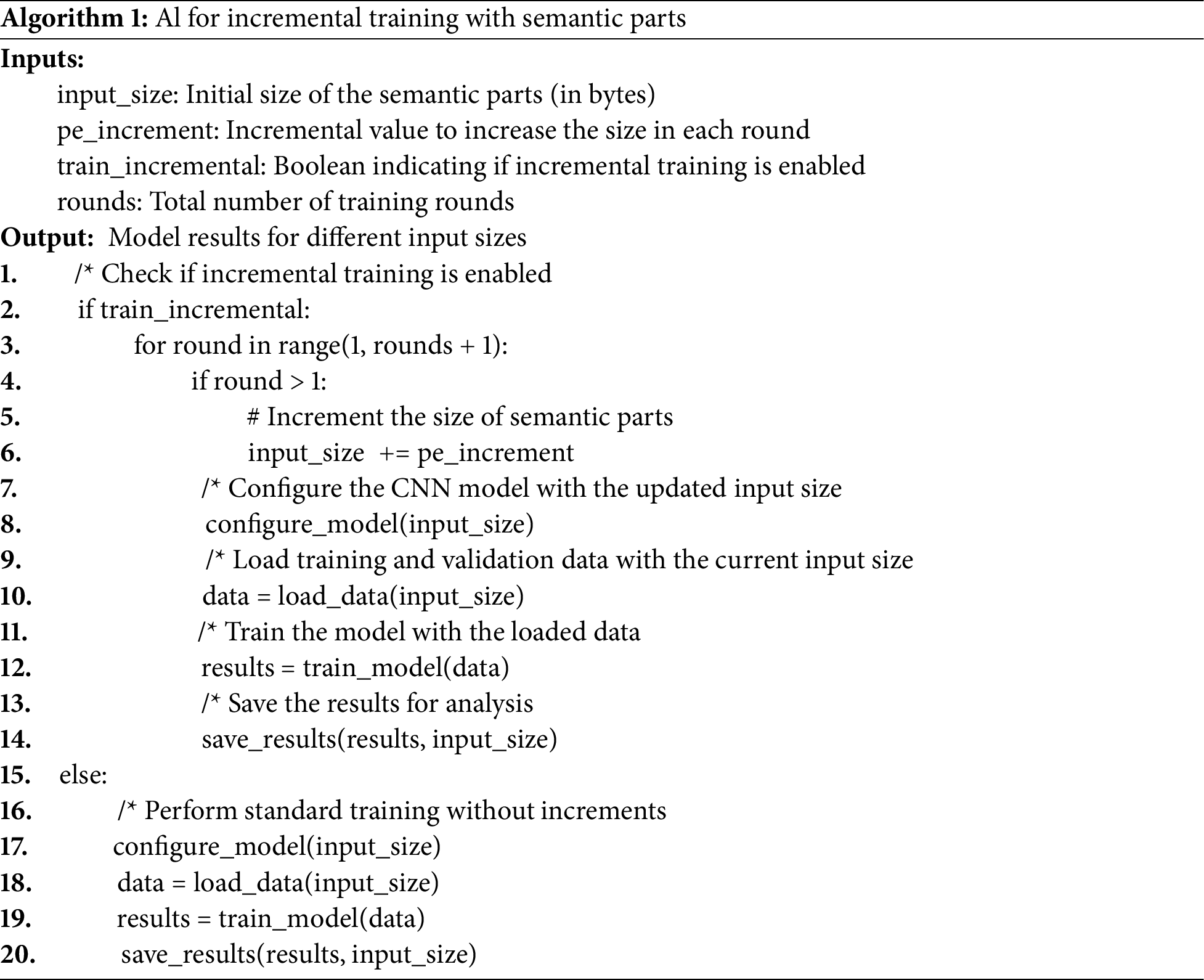
Algorithm 1 is included to improve the understanding of Fig. 8.

This model was chosen to ensure that each step has its dataset created randomly and isolated, thus ensuring the data used for testing and prediction were new to the trained model.

3.4 Metrics and Their Justification

Two metrics were used for global model evaluation: Sparse Categorical Accuracy (SCAcc) and Sparse Categorical Cross Entropy (SCCE). SCAcc calculates how often predictions match the integer labels, while SCCE computes the cross-entropy loss between the labels and predictions provided as integers. Both metrics are calculated using the Keras API in the test data [45].

•   SCAcc checks whether the actual maximum value equals the index of the maximum predicted value by calculating the frequency with which the predictions match the full labels. Accuracy was measured in three phases: training, validation, and evaluation. Training accuracy indicates how well the model learns to map inputs to outputs. Validation accuracy measures the degree of generalization of the network during training. Evaluation accuracy indicates the generalization power on new data once the model is trained.

•   SCCE is the cross-entropy loss function used because the expected result of the classification problem comprises a set of discrete values with nine possibilities.

For the final calculation of the cross-validation result for accuracy and error rate, global model evaluation metrics, Eqs. (1) and (2) are used.

(1)

(2)

The performance of the malware classification approach was evaluated using the metrics accuracy (SCAcc) and loss (SCCE). These metrics were chosen for their suitability in evaluating classification models. Accuracy provides a simple measure of the model’s overall correctness, while loss assesses the model’s ability to generate predictions that align closely with the true labels. Together, they provide a comprehensive evaluation of the model’s performance.

The use of accuracy and loss as metrics aligns with standard practices for evaluating machine learning models, particularly in classification tasks. In addition, these metrics are directly relevant to the research question as they explicitly measure the model’s accuracy in classifying malware.

4  Development and Experiment

4.1 Dataset Structure and Composition

The existence of a dataset of sample malware files in PE format is a prerequisite for performing any research related to malware classification using machine learning (ML) techniques that require static feature extraction. In preparing this dataset, the purpose of the analysis, the sample format, the quantity, the existence of binaries, and the presence of tags are considered as criteria for selection [13].

The database used contains 28.617 malware samples with binary files in PE format labeled into nine families. The original files were compressed without extension to avoid improper execution. They were unzipped only for static feature extraction. The sample information provided with the dataset is composed of two data structures: one containing the list of file names and the other with the labels, related through a common index. The dataset originates from the research work [13], fully provided by the author. Technical details, criteria, and the base creation process are described in Appendix “A” in the author’s thesis.

The reason for choosing the dataset developed by Sant’Ana (one of the authors of this study) lies in its relevance and suitability for the task of malware classification. This database provides a wide variety and representativeness regarding PE file characteristics of malware samples, which allows to effectively train and evaluate artificial intelligence models in an environment that resembles real-world conditions.

In addition, it includes diverse malware families and structural features, which is critical for developing more robust and accurate models. In the first instance, a search for malware datasets publicly available on the Internet was conducted, but none of them had the necessary samples of malware specimens to perform the research. Datasets in .csv format were found but did not have the samples, so they were not useful for the research.

The dataset preparation process involved collecting and labeling malware samples for the VirusShareSant dataset. This process was made by Sant’Ana as part of his doctoral [13].

•   Malware Sample Collection: The malware was selected from 7 sample packages from VirushShare, previously labeled in the ML Sec Project and validated by VirusTotal, which has complete malware samples.

•   Initial Family Selection and Acceptance Criteria: An initial selection of 17 malware families was made, and specific acceptance criteria were applied to each sample. These criteria included being detected by Microsoft antivirus, being detected by at least 10 other antiviruses, and having at least two other antivirus solutions using family nomenclature similar to Microsoft antivirus.

•   Validation of Compatibility: The PEFILE library in Python was utilized to verify if the malware samples were compatible with the Microsoft Windows PE FILE standard. Samples that were not compatible were discarded.

•   Final Family Selection: The final selection of families for the VirusShareSant dataset was made by selecting the nine families with the largest malware samples, resulting in 28,617 samples.

Table 2 presents the data distribution across families, with the percentage representation and weight of each class in the set. The data is unbalanced, with an amplitude difference of about 86% between the smallest value (BrowserModier: Win32/Zwangi) and the largest (Trojan: Win32/Vundo). The two largest classes represent about 44% of all the data.

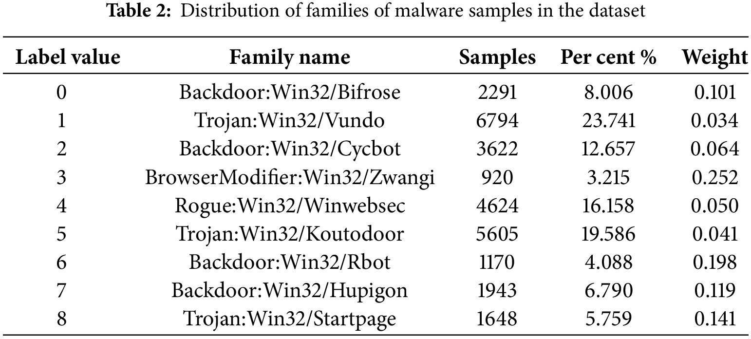
The distortion in the data distribution represents a difficulty for ML algorithms that assume the number of objects in the considered classes is approximately similar. However, in real-life situations, the distribution of examples is often skewed, where representatives of some classes appear much more frequently than others. Nonetheless, the minority classes can be the most important, as they carry valuable and useful information for the domain [45].

An over-sampled version of the dataset was used to address this problem. An algorithm was created to randomly separate data into sets proportionally for training (utilized to train the model), validation (employed to compare different models and hyperparameters), and testing (utilized to validate that the model works, ignored in training and the process of choosing hyperparameters).

The process initially randomly separates 80% for training, and the remaining 20% is randomized and divided proportionally 50% into the other two. This 20% was further randomized and divided equally into the validation and test sets. The pandas.DataFrame.sample() is the primary function utilized to return a random sample of items from the dataset. The split process was repeatedly for each phase of the k-fold cross-validation process. This process is designed to be performed before each model training series.

The proposed method in the study addresses the scalability with larger and more diverse datasets by employing semantic-based segmentation of PE files to reduce the input size required for training, directly impacting the computational resources and training time. The key points from the document regarding scalability and dataset size impact:

•   Semantic Segmentation and Data Limitation: The method separates the PE file into semantic parts (header, code, data) and evaluates the model’s performance using smaller datasets derived from these parts. This segmentation allows effective use of data without requiring the entire file, as observed in their experiment, with headers achieving the highest accuracy (99.54%) using only 4 KB of input data.

•   Impact on Training Time: The research highlights that reducing training data size (using semantic parts) proportionally decreases training times. For example, models trained using header data showed shorter training durations compared to those using full file data, as indicated in their incremental cross-validation results.

•   Generalization Across Dataset Sizes: The method ensures the model’s ability to generalize effectively with varying dataset sizes by adopting incremental cross-validation and limiting data sizes for code, data, and file categories. The use of 114.468 files, generated with constrained byte limits, further validates scalability without compromising performance metrics (accuracy and loss).

Accordingly, the proposed approach demonstrates effective scaling by strategically reducing the input size for training, thus optimizing computational resource usage and maintaining high classification accuracy even with constrained datasets. This consideration of dataset size directly impacts training times and model performance, showing the method’s adaptability to larger datasets.

Of course, if it becomes necessary to use a significantly larger dataset or increase the amount of data processed for each semantic part, a viable alternative to maintaining reasonable and consistent training times will be to adopt more advanced hardware specifically designed for machine learning training. Equipment such as high-performance GPUs (NVIDIA A100 series) or TPUs, which are designed for deep learning operations, can significantly accelerate the training process. In addition, using servers optimized for parallel processing and high-capacity memory will further facilitate handling larger and more complex datasets without compromising training efficiency. This approach will enable the model to scale effectively to accommodate larger datasets while preserving productivity and the expected outcomes.

4.2 Extract PE Features

The data extraction from executable files was conducted statically, relying only on information obtained by reading the bytes stored in the file. These bytes were normalized to values on a hexadecimal scale (integers ranging from 0 to 255) and grouped into four categories: Header, Code, Data, and File (the latter representing the entire file). The term semantic part refers to the elements within these groups.

The semantic variation concept approach involves the static extraction of malware features in Portable Executable (PE) format to feed neural network systems. This approach recognizes that the bytes of a PE file can contain multiple types of information that can be spatially correlated with each other, depending on the section where it is stored.

This approach is utilized to extract data from PE files based on the semantic meanings of the parts of a file to feed the input layer of neural networks to identify characteristics through convolutions. Data extraction from the files is done statically, considering only the information that can be obtained by reading the bytes of files stored in the file systems.

This approach is based on semantic variation for the static extraction of malware features in PE files, to provide data for neural network systems. The bytes of a PE file can encode various types of information, potentially correlated depending on the section in which they are stored. Thus, the data collection respects the semantic nature of each part of the file to feed the input layer of neural networks designed to identify features through convolutions.

PE files comprise a set of headers and sections that store various data types. The number, usage, and attributes of these sections are defined by development tools and programmers based on the desired functionality [46]. At a minimum, a PE file requires two sections to function: one for code and another for data. Although standard section names and functions are commonly used, there is no restriction against using alternative names, particularly in obfuscation techniques. A complete list of standard sections is available in [47]:

1.    Executable code section (.text)

2.    Data section (data, .rdata, .bss)

3.    Resources section (.rsrc)

4.    Data export section (.edata)

5.    Import data section (.idata)

6.    Exception handling functions section (.pdata)

7.    Debugging information section (.debug).

The sections are defined in a data structure known as the section table, where each row represents a 40-byte section header. The last 4 bytes of each header store the section’s characteristics, which indicate the type of content or actions the section can support. Table 3 outlines some of the relevant characteristics of this study; the complete list can be found in [47].

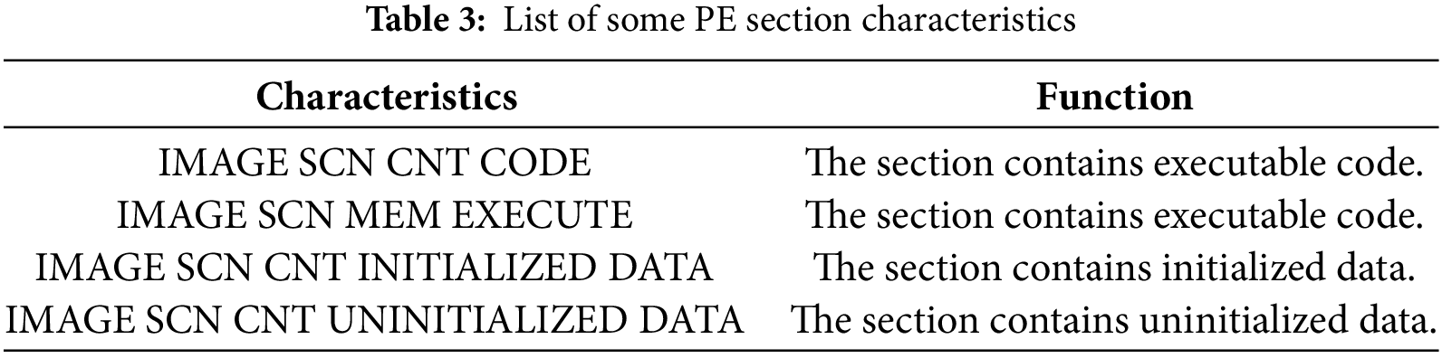
Identifying code and data sections as semantic parts was based on these characteristics. For code sections, CNT_CODE and MEM_EXECUTE were utilized to indicate the presence of executable code, while CNT_INITIALIZED_DATA and CNT_UNINITIALIZED_DATA were applied to identify sections containing data. A section was classified as either code or data if it exhibited at least one of these characteristics.

The extraction of byte sequences based on semantic context involves reading the file and padding the sequence with zeros when the byte count is below the desired limit. The bytes are then normalized to integers from 0 to 255. The boundaries for each category are defined as follows:

•   Headers: These are well-defined structures in PE files. The sizeof_headers property indicates the total size of the headers, enabling their extraction.

•   Code and Data Sections: These are identified using the characteristics CNT_CODE, MEM_EXECUTE, CNT_INITIALIZED_DATA, and CNT_UNINITIALIZED_DATA. A section is classified as either code or data if it contains at least one characteristic of the respective category. Although this method is not infallible, it has proven effective in identifying the parts necessary to characterize the semantic content of a PE file.

A control mechanism was implemented to prevent any section from being simultaneously categorized as both code and data in cases where properties overlapped to ensure accurate classification. Although it is acknowledged that all information within PE files can potentially be manipulated, no viable alternative for automating the static identification and separation of sections was identified. As a result, this approach was determined to be the most effective and practical solution for achieving semantic segmentation of code and data.

Data were collected for all features of all sections in the files, resulting in a set of 148.815 rows and 37 columns to verify whether the proposal of using features to separate codes and data can be implemented. The rows represent the total number of sections in all samples, and the columns represent the number of features found in the sections. From the result of overlapping the collected data, grouped by files, sections, and characteristics, it can be inferred that all files have at least one section with one of the four characteristics used, and the criterion can be considered valid.

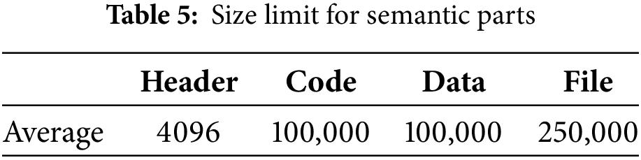
After defining the data separation process, statistical data of the sizes of all semantic parts of the samples were collected to evaluate the possibilities of limiting the sizes of the sequence of bytes to be extracted. The results are listed in Table 4. The definition of limits was necessary, firstly, to limit the amount of extracted data because it directly impacts the use of computational resources, and secondly, for planning purposes of defining the input dimensions of the CNN models.

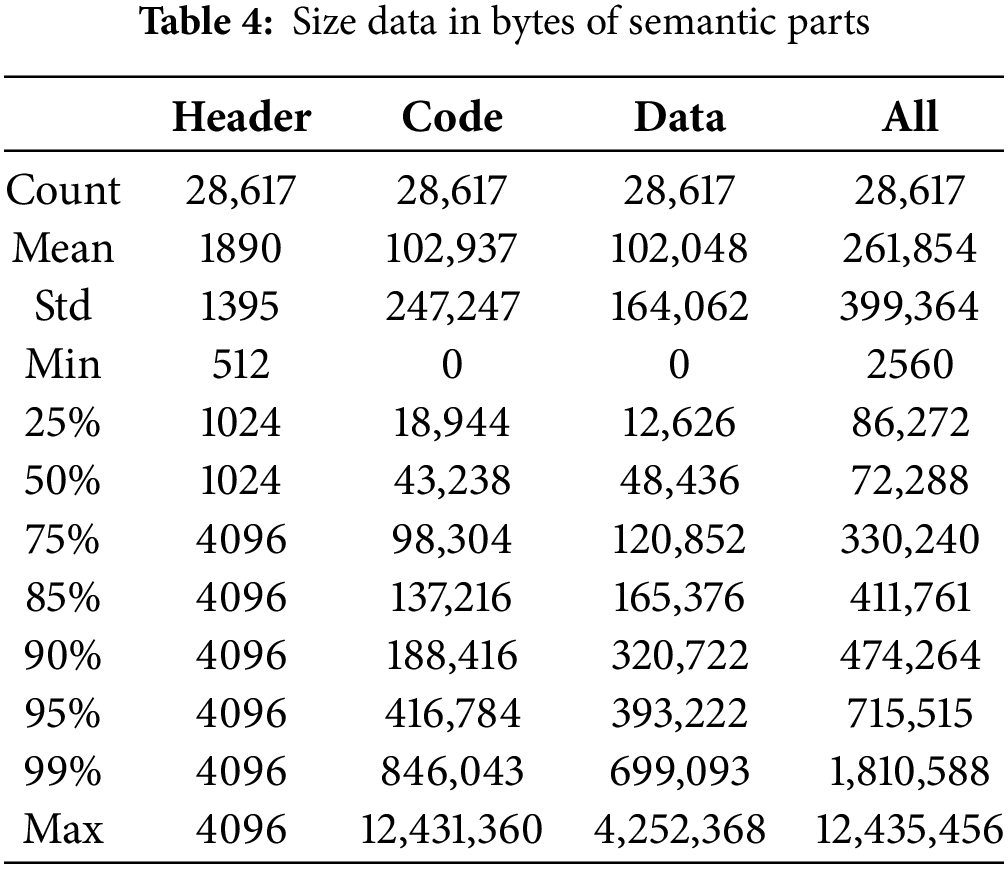
The maximum observed header size was 4096 bytes for all samples, and this value was utilized to define the size of the sequence to be extracted. For codes, data, and files, it was decided to use an approximation of the average values as a feasible value considering the computational resources available, limiting respectively to 100,000 bytes for codes and data and 250,000 for the file.

For each of the semantic parts, a new file was generated for each of the samples with the size of the defined maximum limits. If the amount of data was smaller than the limit, the sequence was completed with zeros. The 114,468 files generated containing the byte sequences in decimal scale in the format of a NumPy array were stored on disk. The UINT8 data type was utilized to store the byte values as unsigned integers to reduce storage space and memory footprint during neural network training.

The Leif library was utilized to implement the logic for extracting the data from the malware samples. The library provides a common abstraction via API for performing analysis and modification on executable files of various formats, with support mainly for the languages C++ and Python. It also supports various executable file types. With this library, it is possible to retrieve all the contents of the header from a property that provides the total size of the headers. The bytes are extracted from the beginning of the file to the maximum value defined, completing with zeros where necessary.

The algorithm processes all the file sections to check the characteristics and aggregates the extracted content sequentially until the maximum limit is reached to extract the code and data sections. After extraction, it is impossible to identify the data’s origin.

The extraction of bytes for the part called file, which represents the entire file, was performed based on the original proposal of the Malconv model [9], from the beginning of the file to the maximum defined limit. The original model used about 2,000,000 bytes, and this study employed 250,000 due to computational resource limitations.

Examples of data processed from headers and loaded into RAM (a) with their labels (b) are illustrated in Fig. 9. All extracted semantic parts have the same representation format, changing only the second value of the dimension representing the sequence size.

Figure 9: Representation of extracted semantic part data: (a) headers loaded into RAM; (b) with their labels

4.3 CNN Architecture

The present research, in terms of neural network architectures, aims to solve the problem of classifying samples of binary files in PE format into families using supervised learning techniques. Fig. 10 shows an overview of the proposed use of CNNs in this work, which consists of using the same network architecture with semantic data extracted from PE files to classify samples into families. It emphasizes the extraction of components from Portable Executable (PE) files (Header, Code, Data, File) and their input into a pre-trained CNN model, which then classifies the input into one of the predefined malware families.

Figure 10: Overview of how CNN works

The choice of the CNN architecture over other effective classical machine learning systems, such as Support Vector Machines (SVM), is based on the work by Edward Raff et al. [9], which justifies the application of neural networks to malware detection due to their generalization properties on unknown data using features of malicious PE files.

In addition, CNNs are particularly well suited for processing data with multiple dimensions, such as the raw bytes of malware files in PE format. The structure of CNNs makes it possible to efficiently extract features and discover complex patterns from large data sets.

Using CNNs provides several advantages over traditional malware detection methods. These include the ability to automatically learn and adapt to new malware variants, the potential for higher accuracy compared to standard signature-based methods, and the capability to detect zero-day threats unknown to traditional security systems.

The research focused on CNNs due to their demonstrated effectiveness in image recognition and natural language processing tasks, which involve similar challenges in terms of pattern recognition and feature extraction. In addition, previous studies have shown promising results using CNNs for malware detection in PE files.

This study does not propose a new CNN malware detection or classification architecture. However, it relies on one to perform practical research activities. Thus, an architecture for malware detection created by Edward Raff et al. [9], called MalConv, was used for the detection of malware. Fig. 11 is a graphical representation of this preexisting model. It can be visualized as two representations of the model with different levels of abstraction, in (a) an overview as defined by [9] and in (b) an extended representation of [42].

Figure 11: Malconv representation: (a) overview; (b) an extended representation (Source: Raff et al., 2017 [9]; Demetrio et al., 2019 [42])

A detailed analysis of the MalConv architecture to understand how the system learns to discriminate between malicious and benign executables using raw bytes can be found in the literature [48], where the gradients at various stages of the trained network are analyzed to see how the system assigns weights to different parts of the executable, among other technical features. The MalConv model was selected based on the following criteria:

1.    It was one of the first malware detection initiatives that used raw neural network input bytes extracted sequentially from PE files, without any additional processing, for feature selection with the ability to generalize [49].

2.    There are some publicly available implementations of the architecture, making it possible to understand and allowing for reuse.

3.    It uses a sequence of raw bytes of fixed size, selected from the start of the file to the defined boundary, as input to the neural network. This type of input and the characteristics of the neural networks are compatible with the proposal of this research, visualizing a possibility of comparing results by performing the MalConv training with the database of this work.

4.    The architecture was used in several works such as Coull et al. [41] analyzed a deep neural network model for malware classification, Ling et al. [2] studied ML/DL methods for malware detection PE, Vinayakumar et al. [7] addressed the use of CNN and Recurrent Neural Networks (RNN) with long term memory (LSTM) for malware detection, Gibert et al. [21] performed a survey on machine learning for malware detection, Jeong et al. [25] proposed a CNN to detect malware in byte streams of PDF files by extracting spatial patterns, Burr [49] used Malconv model for malware detection, Demetrio et al. [42] explained DL vulnerabilities, Anderson et al. [50] addressed malware classification using LSTM language models. Finally, Raff et al. [8] indicated that the Malconv model is the most efficient for performing malware classification and detection tasks.

5.    It provides an opportunity to add some semantic context to the architecture. Demetrio et al. [42] indicated that MalConv learns to discriminate between benign and malware samples primarily based on file header characteristics, almost ignoring the data and code sections where the malicious content is usually hidden. This also means that, depending on the training data, it can learn a spurious correlation between class labels and how file headers are formed for malware and benign files.

In addition, the CNN architecture was adapted to learn efficiently from statically extracted raw byte sequences by performing the following tasks:

1.    Semantic Segmentation: The PE files were split into different sections based on meaning. Different parts of the file (such as headers, code, and data) do different things and will have different byte patterns.

2.    Static Data Extraction: Raw byte sequences were extracted from each section (with some limits due to malware sizes). This way, this study only looks at the structure of the PE file, not how it runs.

3.    Preservation of Semantic Context: The context is kept by taking byte sequences from specific parts of the PE file. The CNN sees byte sequences that accurately show the different functional areas inside the PE file.

4.    Leveraging Convolutional Neural Networks (CNNs): CNNs are great for learning from these segmented byte sequences. The convolutional layers can spot patterns within each sequence, capturing the unique features of headers, code, or data sections.

5.    Model Optimization: The CNN was tweaked using techniques such as regularization and the right number of training rounds. This helps prevent overfitting (where the model only works well on the data it’s seen before) and makes it better at handling new PE files.

Performing these tasks ensured that CNNs learned the specific byte patterns of different parts of the PE file, which makes malware classification better and faster.

Fig. 12 presents an adaptation of the MalConv model, inspired by the implementation from [51], for malware classification tasks into families, implemented with the Keras library, to meet the goals of this research. The last layer of the model was changed from a binary output, which was originally designed for the classification of malware into benign and malignant, to a multiple-class output with nine possibilities, corresponding to the nine malware families

Figure 12: MalConv model adaptation code

Fig. 13 depicts the result of compiling the model from the code of Fig. 12 using head-end training data. It indicates that all connected layers of the model, the dimensions of the inputs and outputs, and the activation functions applied. It represents the MalConv model after its compilation and provides a clear visualization of the connections between layers, input and output dimensions, and the activation functions applied at each layer. This approach was chosen to facilitate the understanding of the model’s architecture and its data flow.

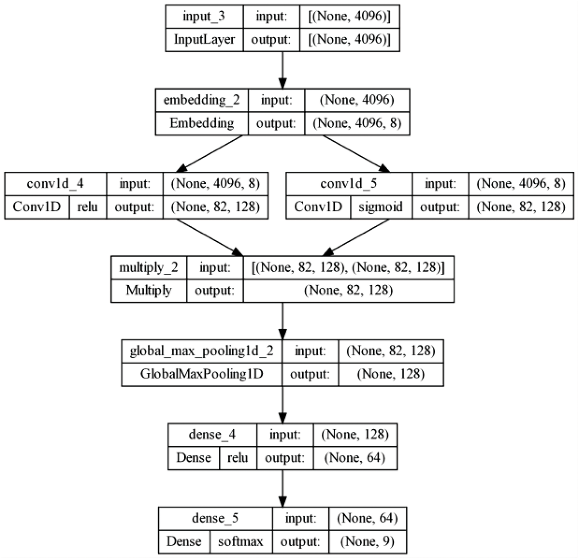
Figure 13: Representation of the compiled MalConv model

In order to improve the understanding of Fig. 8, Algorithm 2 is included.

The first layer of the model represents the data entry point through the Input object, where the linear sequences of raw bytes extracted from PE files have as a parameter the length of the sequence based on the limits in Table 5.

In the second layer, the inputs are transformed into two-dimensional matrices in preparation for the convolution layer. The original model used the Malicious method for the convolution layer. The original model used the MalConv method to perform this transformation, but the Keras library provides the Embedding API to perform this process.

The Embedding layer transforms a one-dimensional input into a two-dimensional output based on two main parameters: the size of the representative vocabulary of the data types and the value of the expansion dimension.

Next, the model uses two one-dimensional convolution layers (Conv1D9), a multiplication layer (Multiply10), a global max-pooling layer (GlobalMaxPooling1D11), and two fully connected layers (Dense12). Conv1D convolutions use convolution windows on the input value of the layer in a single spatial dimension to produce outputs based on the number of filters applied.

The Multiply layer is a data binding layer that multiplies the values of the input lists. It takes as input a list of data structures in the same format and returns a single structure in the same format. The GlobalMaxPooling1D layer performs a global max-pooling operation for temporal data, reducing the input representation to the maximum value size in the time dimension. This network’s temporal dimension is represented by the number of filters generated in the convolution layers.

The Dense layers are the fully connected layers of the model. Two layers are used: the first receives the clustering output as input, and the second one, connected to the first one, condenses the output into nine possible classes. The last layer of the model was changed from a binary output, originally designed to classify malware into benign and malignant, to multiple class outputs with nine possibilities corresponding to the nine malware families. Due to using a categorical variable to represent the discrete domain of the labels, the activation function SoftMax was employed.

In the convolution and fully connected layers, only the values considered hyperparameters of the algorithm were changed. The selection process and values used for these hyperparameters are discussed in the following sections.

4.4 Hyperparameters

The model was compiled with the sparse categorical accuracy metric and the cross-entropy loss function to measure accuracy and loss in training and validation, respectively. The accuracy metric calculates how often the predictions match the labels. The higher the value, the better the model.

The loss function quantifies the penalties incurred when the label estimate does not exactly match the predicted one. The lower the value, the better the model. The Stochastic Gradient Descent (SGD) algorithm was used as the optimization technique, with the same parameters as the original proposal of the MalConv model. Stochastic Gradient Descent is an optimization algorithm often used in machine learning applications to find the model parameters that correspond to the best fit between predicted and actual outputs. The application of the metric configuration and the optimization algorithm are illustrated in Fig. 14.

Figure 14: Metrics tuning and optimization

The number of filters and units in the penultimate Dense layer was kept per the reference implementation. The kernel size was changed for the header data to 50 bytes due to the maximum size of 4096, as using 500 bytes in the convolution window did not yield the expected results.

The number of epochs is a hyperparameter that denotes the number of times the learning algorithm will be run on the entire training data set. Iteration over the dataset is performed in batches of configurable size. The number of epochs used as a MalConv model indicated in the literature ranges from 5 in the tests of application of Dropout layers in [52] and up to 1000 [7]. Different databases were used in all cases where the number of seasons was indicated.

The EarlyStopping technique was used for regularization in statistics as no reference patterns were found to control the number of epochs in training [53]. It is a form of regularization based on choosing when to stop running an iterative algorithm. Fig. 15 presents an example of applying this technique to stop training with header data when the validation accuracy reaches a value of 0.982 and is held stable for 20 epochs while the training accuracy continues to increase.

Figure 15: Example of the early stop operation

One of the goals of employing this technique is to avoid overfitting, a phenomenon pervasive in all statistics, as well as to reduce computational complexity [54]. The same configuration pattern was maintained for all the training performed in this research work. Each training series can be performed for up to 1000 epochs, using the validation accuracy metric as a parameter for applying the technique, considering the sequential results of 20 epochs without improvement in the metric values. The EarlyStopping API was utilized to implement the technique.

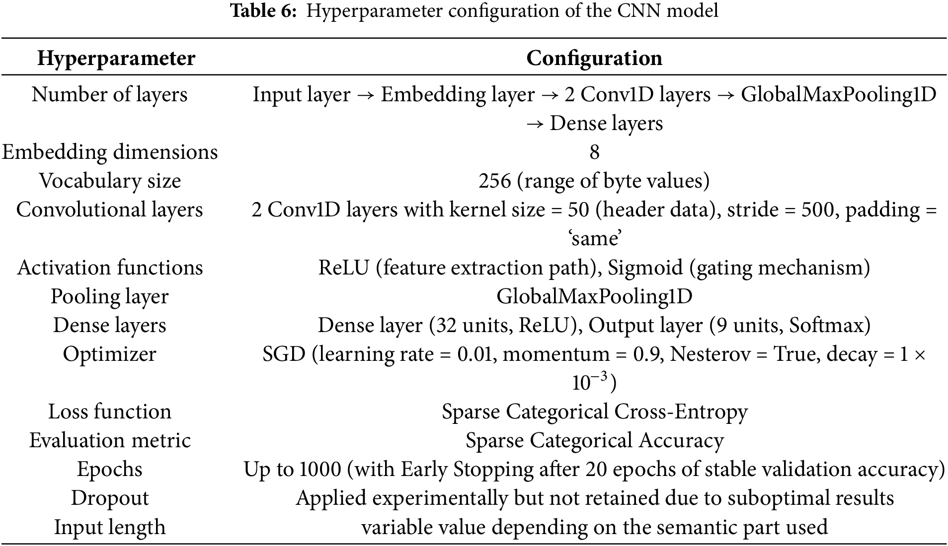
Table 6 summarizes the hyperparameters of the AI model used in the research:

4.5 Tests and Verifications Performed

The problem of classifying malware into families is an example of supervised machine learning, where the model is trained from examples that contain labels. Evaluation occurs with the trained model, which uses the test dataset with its labels to determine how well the model predicts. Based on the proposed incremental cross-validation method, training was performed with data from the semantic parts, gradually increasing the number of bytes of the sequences between training runs.

Due to the maximum size of the headers, using the incremental technique was unnecessary. Six runs were performed with the value of 4096 bytes of input. For codes, data, and files, the sequences were incremented by 5000 bytes by default between runs up to 25,000, with this value doubled for the last run. The initial value of 5000 was chosen because it represents the dimensional space for ten standard convolution windows of the original MalConv model and allows flexibility in choosing the values up to the maximum limits available.

Each training run began by randomizing and separating the data into three sets (training, validation, and testing), loading the data from disk to machine memory, training the model for the maximum number of defined epochs (or until early stopping), evaluating the model with the testing data, and performing predictions on the testing data to validate the generalizability of the model. Using the same dataset in the last two steps does not cause interference because, during evaluation, the model no longer learns from the data.

The models were trained in the semantic parts with the Keras API fit method, and all the datasets were loaded into RAM. The training results were grouped by parts in Tables 7–9. Each table contains the number of the test series, the epoch where the best training result was obtained (from this point on, the epochs were counted using the early stopping technique), and the values of the accuracy metrics (SCAcc) and the loss function (SCCE) for training, validation, and evaluation. The result of the predictions is represented by the percentage of correct predictions.

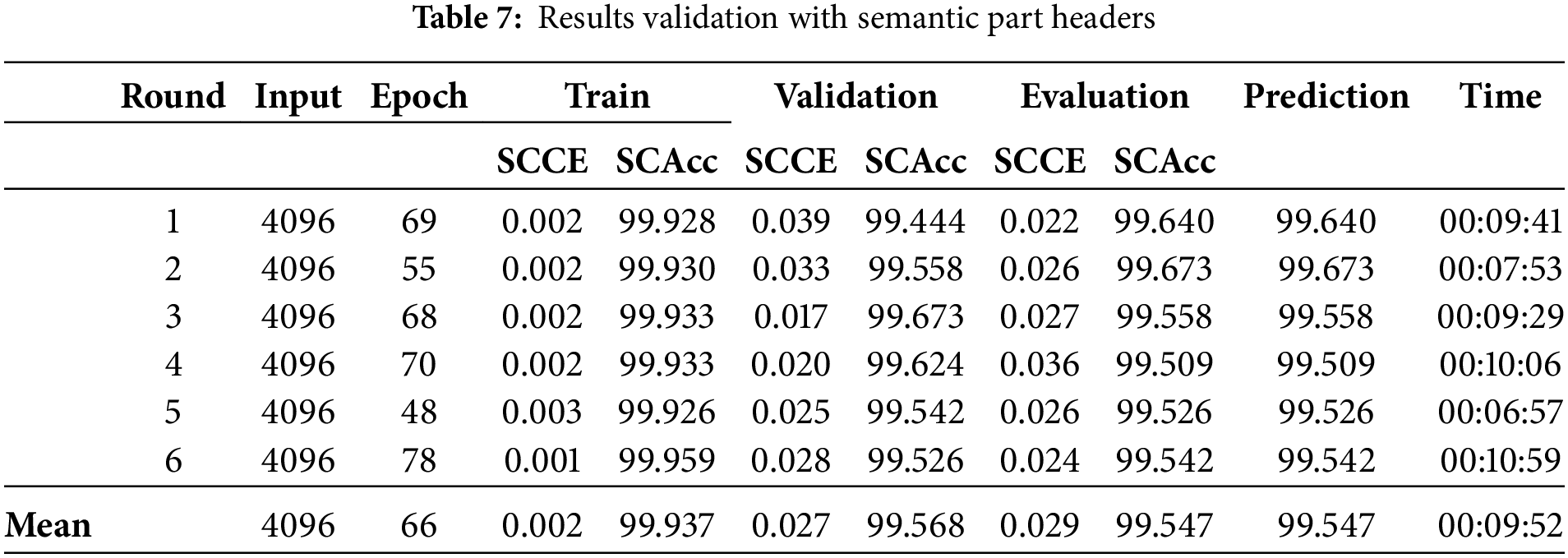
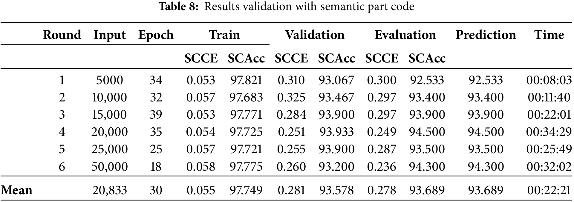
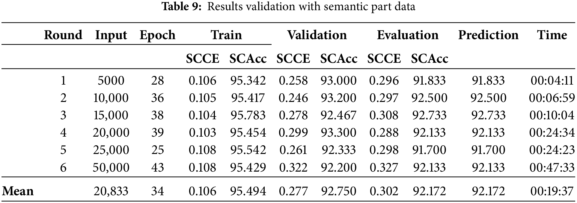
The execution times for each run are expressed in the last column and represent the total time until the predictor completes the run. The averages of the results are calculated in the last row based on Eqs. (1) and (2). These values are used for analysis and comparison to other results.

5  Results and Discussion

This section presents the results obtained from the tests and compares them to results from other research. Tables 10 shows the validation of the results of the whole file.

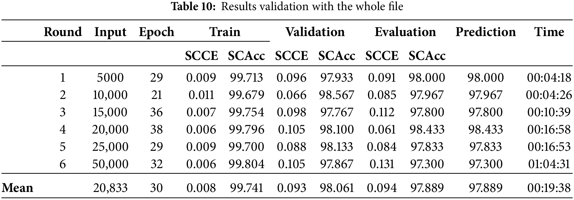
Analyzing the results of applying the incremental cross-validation method indicates that the expected effects related to obtaining similar performance using fewer data and using the same random data between the series were achieved. Thus, the first hypothesis is validated by obtaining the same performances as the models trained with more input data in shorter times.

The reduction in training time was directly proportional to the amount of input data in the time dimension of the convolutional layers, which in the applied case is the number of bytes. The more data, the longer the time, considering that the same number of samples and fewer hyperparameter values were used. Fig. 16 shows the comparisons with the four semantic parts considered. The results of the headers are linear because the input was the same for all runs.

Figure 16: Relationship between validation and input size

Fig. 17 shows the relationship between the number of bytes and validation accuracy. It demonstrates that the increase in data does not improve the accuracy, with a slight reduction in the semantic part of the data.

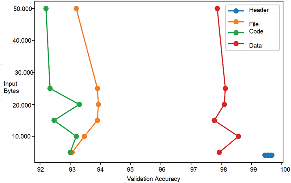
Figure 17: Relationship between the number of bytes and validation accuracy

Comparing the results of the four semantic parts demonstrates that the use of headers provides the best results in all the evaluated input sizes, with an average evaluation accuracy of 99.54%. Considering the small amount of data used, with only 4096 bytes, the average time spent in training, and the accuracy of the results. This conclusion collaborates with the observations of [42] that the MalConv model learns much more from the header data than the rest of the data in the other sections.

The second-best result was obtained in the non-semantic part (although in the scope of this work, it is called semantic for standardization purposes), using the all-byte sequence, with an evaluation accuracy of 97.88%, followed by data with 92.17% and code with 93.68%. This result is likely because the all-byte sequence contains all the header data. This is most evident with the results of the first training run in Table 8, where when only the first 5000 bytes of the file stream are used, the headers account for about 80% of the data.

For the semantic parts of the code and the data in Fig. 18, a possible case of overfitting occurred, where the curves of the metrics are far apart at the beginning of the training and do not converge again. The hyperparameters of the model will probably be modified to address this situation. However, as one study aims to compare results with the same set of parameters, no changes were made. Perhaps this is also related to the observations of Demetrio et al. [42] that the model does not learn from features in other areas of the PE files.

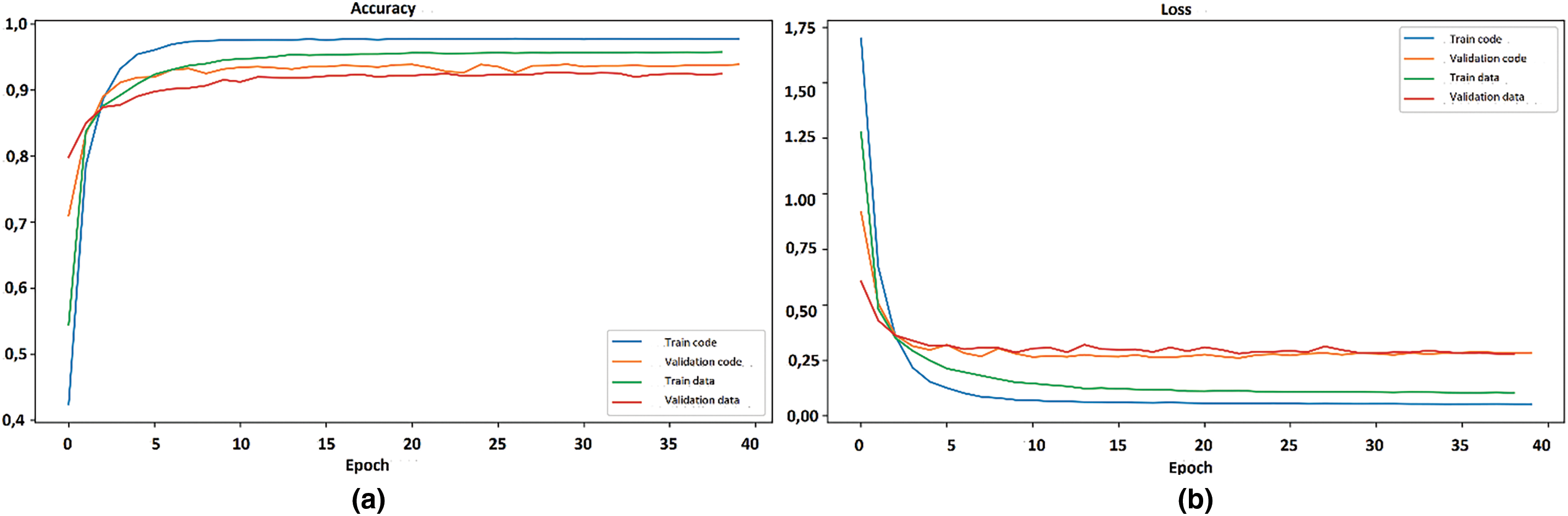
Figure 18: Best results for code and data: (a) Accuracy, (b) Loss

Tables 11 and 12 provide complementary insights into the performance of the proposed CNN model for malware family classification. Table 11 presents the average results across all semantic parts during cross-validation, while Table 12 highlights the model’s performance with the smallest input data (5000 bytes) for each semantic part.

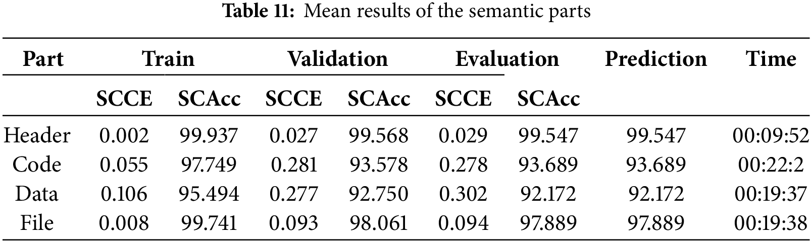
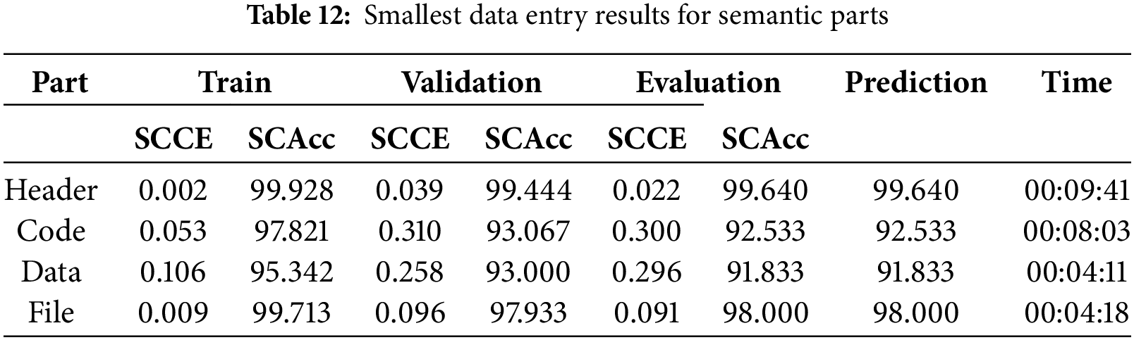
The comparison of results from both tables reveals a strong consistency in the model’s accuracy (SCAcc) across the training, validation, and evaluation phases, even when the input data size is significantly reduced. The differences in SCAcc values are minimal, particularly for the ‘Header’ and ‘File’ semantic parts, with variances below 0.2 percentage points. This indicates that the model demonstrates robust generalization and can effectively classify malware families with limited data input.

In addition, the SCCE values remain low across both scenarios, further confirming the stability and reliability of the model. These findings imply that CNN does not require extensive input data to achieve high classification accuracy, which can reduce computational overhead and facilitate deployment in resource-constrained environments.

The second comparative analysis was performed with the author’s results of the semantic variation problem [13]. In his proposal for solving the problem, the author used the representation of the semantic parts as images, using Lenet-5 Tiny for the header and VGG16 non-top for code and data. Table 13 shows the compiled results, considering the highest value obtained by the author in the test or validation accuracy metric with the average values found.

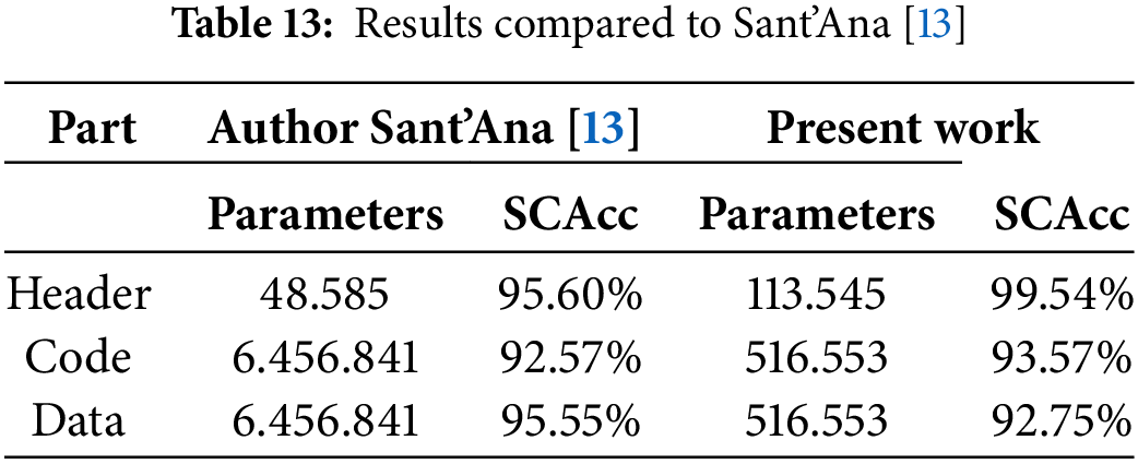
In the validation accuracy for headers, the model improved by about four percentage points, but with about 35% more trainable parameters. In the results for codes, an improvement of one percentage point was also obtained, but with only about 8% more trainable parameters. No better results were obtained for data but with only about 8% more trainable parameters. The best results are highlighted in bold.

The third comparative analysis was performed using the results of the author of the MalConv model [9]. Although a direct comparison cannot be made, firstly because of the classification category used since the original model was a binary classification and the one used in the present research is multiple classifications, and secondly because the author only tested raw byte sequences from the whole file.

It will be possible to make a rough comparison to have an overview of the model’s performance without and with the semantic context applied. Hence, only the best of the results obtained by the author in the Area Under the Curve (AUC) calculations were considered, a measure he utilized to assess the model’s best performance in distinguishing between positive and negative classes. The results of Raff et al. [8] were compared to the average of the results in the semantic parts to visualize the model’s overall performance (Table 14).

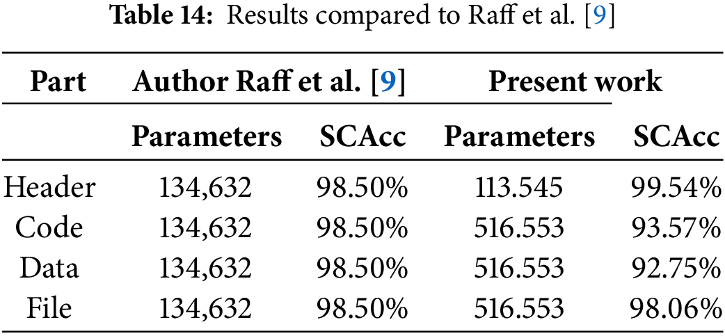
The results of the models used in the present research were compared and analyzed with models trained in similar research, obtaining an improvement in malware classification accuracy between 1% and 4%”.

The fourth comparative analysis is the comparative analysis of the research articles reviewed in the literature review regarding malware detection and analysis. Table 15 shows the result of this comparison:

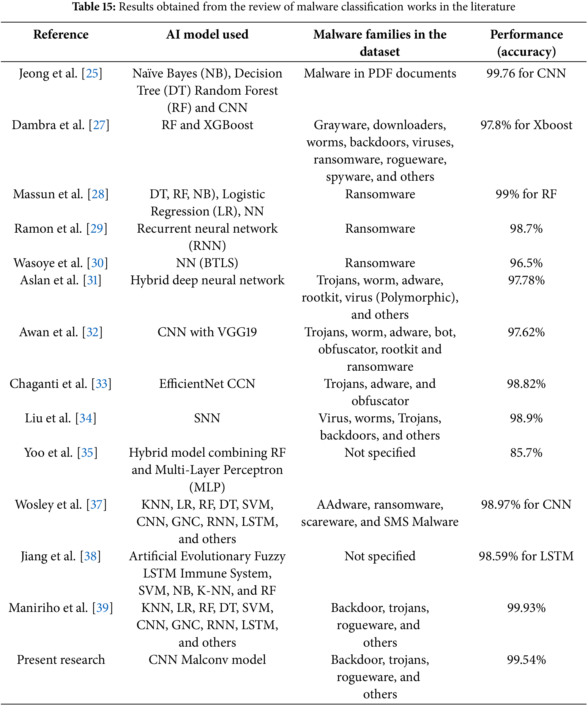
Table 15 indicates that the best performance in the classification of malware was obtained by Maniriho et al. [40] with an accuracy of 99.93% in a specific dataset. It should be noted that the same AI model (CNN) obtained an accuracy of 95.73%, 96.16%, and 98.18% on three other datasets. The present research obtained a similar performance to the previous work with an accuracy of 95.54%. Note that the work of Maniriho et al. [40] obtained a lower accuracy in three datasets than the work of the present research, which implies that a better comparison of the two models should be conducted with the same dataset to have more conclusive results.

The result obtained in the work of Jeong et al. [27] is not comparable with that of the present research because it was performed for a dataset composed of malware pdf documents that is very different from the other works developed with a malware PE file families dataset. There are three works developed for the detection and classification of ransomware; the work of Ramon et al. [31] is the one with the best performance with an accuracy of 99%.

The comparative analysis highlights the need for semantic segmentation in datasets to enhance the interpretability and generalizability of results. The present research introduces semantic segmentation as a unique contribution, separating PE files into functional parts to improve classification performance and reduce model complexity.

The results were generally better only when the number of trainable parameters was fewer, except for the header, where more parameters were used than in the original MalConv model. The data presented in this section indicates that results using only header data can be the most representative of a PE file and are the best overall, both in terms of performance and accuracy. The best results are highlighted in bold.

This is because the PE file header contains crucial information about the file’s structure, entry point, and dependencies. The superior performance observed when using headers for classification can be attributed to the following factors:

•   Unique Signatures: Malware families often have distinctive header patterns or signatures, which machine learning models can detect effectively.

•   Compact Information: Headers provide a concentrated source of information relevant to malware classification, enabling efficient learning without the overhead of processing the entire file.

•   Metadata for Classification: The metadata presented in headers, such as the compiler version or timestamps, can be useful for malware classification.

6  Conclusion and Future Works

The execution of this work presents several challenges and limitations. The first is related to the lack of a public and standardized dataset to conduct malware research using neural networks and facilitate comparison and verification of the results, considering that each uses its approach to build its foundations. The availability of malware is a serious problem, mainly due to its role as a cyber weapon.

However, without standardization, the general perception is that research is limited, results cannot be replicated, and comparisons are difficult to make. The need for binary sample files imposes additional challenges to the research. The realization of this research was made possible by previous work [13].

A second is related to the computational resources available to train neural network models. This activity is currently practically unfeasible, given the availability of GPUs and large storage spaces. This can be considered a premise for research planning. Initially, more tests were considered to be performed to better consolidate the results, but during the development of the work, it was perceived that this would not be possible due to the limited time required to perform the activities and the computational resources available.

It can be concluded that they were achieved regarding the fulfillment of the objectives proposed in this research work. The first objective was specifically addressed through the work conducted in the ‘Background and Related Work’ section, with the construction of a theoretical foundation that, although summarized, supports the research. The second objective can be considered accomplished in Sections “Dataset” and “Extract PE Features,” with the reuse of a dataset built with well-defined criteria for the classification of malware and with the activities conducted for balancing the samples in the families.

The third objective is demonstrated in Section “CNN Architecture” with the presentation of the considerations and process for identifying and separating the files based on the characteristics of the sections. The fourth objective is achieved in the Section “Hyperparameters” with an adaptation and explanation of how the Malconv model works to produce multiple classification results. The fifth objective is reached in Sections “Tests” and “Results” where the data collected and comparisons with other results are discussed.

A point that can be considered positive regarding the implementation of neural networks is the existence of libraries that abstract away the mathematical complexity involved in the implementation and operation of algorithms, such as the Keras library used in this work. This allows the researcher to focus on the activities, allowing for better productivity and leaving the complexity of the algorithms to specific research areas.

The use of raw bytes extracted from different parts of PE files (semantic parts) can significantly impact the improvement of pressure in malware classification and detection using CNN architectures in applied research. This conclusion is supported by the test results, which show a substantial influence of the header data on the results, with an accuracy of 99.54% in malware classification. In addition, the results of the models used in the present research were compared and analyzed with models trained in similar research, and an improvement in malware classification accuracy of between 1% and 4% was obtained.

The implications of this finding for future research can be significant, indicating that prioritizing the analysis of PE headers can lead to more efficient and accurate malware classification systems. Future research directions can include:

•   Header-Specific Models: Developing machine learning models specifically designed to extract and analyze PE headers’ features.

•   Ensemble Methods: Combining header-based classification with models that analyze other parts of the PE file to improve overall accuracy.

•   Dynamic Analysis: Integrating static header analysis with dynamic analysis techniques that examine malware behavior during execution.

The results indicate that using data extracted from PE files based on the proposed semantic approach can reduce the computational resources required for model training and produce satisfactory performance results. In absolute values, the smallest amount of data used presented the best results as a resource for machine learning using CNN.

Finally, the main findings and contributions of the study can have several implications for improving future malware detection and classification systems:

•   Improved accuracy: Trained models using convolutional neural networks (CNNs) can lead to increased accuracy in malware detection and classification, which can reduce the number of false positives and negatives.

•   Adaptation to New Threats: Systems can quickly adapt to new malware variants by employing machine learning techniques, which is crucial in an environment where threats are constantly evolving.

•   Analysis efficiency: Automating the detection and classification process using artificial intelligence models will enable faster and more efficient analysis of large volumes of data.

•   Development of New Strategies: The strategies proposed in the study can inspire the development of more robust and versatile malware detection and classification approaches that combine deep learning techniques.

Accordingly, the results of this research can significantly influence the future of cybersecurity, raising the use of advanced technologies to strengthen defense against malware.

Three proposals for future work are indicated based on the results and challenges found in this work. The first relates to applying the semantic proposal in other datasets, either for binary classification purposes or other multiple classification categories, to verify if the results are compatible with those of this work. The second is to validate the process of identification and extraction of sections from PE files to assess the degree of accuracy of the process and whether it is possible to use other techniques in addition to the use of features to identify them automatically and statically and the third the extension of this model for malware classification and detection on Linux systems with ELF file format.

Acknowledgement: Not applicable.

Funding Statement: The authors received no specific funding for this study.

Author Contributions: The authors contributed to the research as follows: conceptualization, Eliel Martins, Javier Bermejo Higuera, Ricardo Sant’Ana; methodology, Eliel Martins, Javier Bermejo Higuera, Ricardo Sant’Ana; validation, Juan Ramón Bermejo Higuera, Juan Antonio Sicilia Montalvo, Diego Piedrahita Castillo; formal analysis, Eliel Martins, Javier Bermejo Higuera; resources, Ricardo Sant’Ana; data curation, Eliel Martins; writing—original draft preparation, Eliel Martins, Javier Bermejo Higuera; writing—review and editing, Eliel Martins, Javier Bermejo Higuera, Juan Ramón Bermejo Higuera, Juan Antonio Sicilia Montalvo, Ricardo Sant’Ana, Diego Piedrahita Castillo; visualization, Eliel Martins, Javier Bermejo Higuera, Juan Ramón Bermejo Higuera, Juan Antonio Sicilia Montalvo, Ricardo Sant’Ana, Diego Piedrahita Castillo; project administration, Juan Ramón Bermejo Higuera, Juan Antonio Sicilia Montalvo, Diego Piedrahita Castillo. All authors reviewed the results and approved the final version of the manuscript.

Availability of Data and Materials: The dataset codes are available at https://github.com/ricksant2003/MalwareDatasetVirusShareSant (accessed on 20 January 2025). The code created for database treatment, feature extraction from PE files, training and evaluation of neural network models, and analysis of the results are available at https://github.com/elielmartinsbr/semantic-pe-cnn (accessed on 20 January 2025).

Ethics Approval: Not applicable.

Conflicts of Interest: The authors declare no conflicts of interest to report regarding the present study.

References

1. Jang-Jaccard J, Nepal S. A survey of emerging threats in cybersecurity. J Comput Syst Sci. 2014;80(5):973–93. doi:10.1016/j.jcss.2014.02.005. [Google Scholar] [CrossRef]

2. Ling X, Wu L, Zhang J, Qu Z, Deng W, Chen X, et al. Adversarial attacks against windows PE malware detection: a survey of the state-of-the-art. Comput Secur. 2023;128(3):103134. doi:10.1016/j.cose.2023.103134. [Google Scholar] [CrossRef]

3. He K, Kim DS. Malware detection with malware images using deep learning techniques. In: 2019 18th IEEE International Conference on Trust, Security and Privacy In Computing and Communications/13th IEEE International Conference on Big Data Science and Engineering (TrustCom/BigDataSE); 2019 Aug 5–8; Rotorua, New Zealand. p. 95–102. [Google Scholar]

4. AV-TEST. Malware and PUA Dashborad (2024). 2024 [cited 2024 Jan 10]. Available from: https://portal.av-atlas.org/. [Google Scholar]

5. Cozzi E, Graziano M, Fratantonio Y, Balzarotti D. Understanding linux malware. In: IEEE Symposium on Security and Privacy (SP); 2018 May 20–24; San Francisco, CA, USA. p. 161–75. [Google Scholar]

6. Yamaguchi S, Gupta B. Malware threat in Internet of Things and its mitigation analysis. In: Research anthology on combating denial-of-service attacks. Hershey, PA, USA: IGI Global; 2021. p. 371–87. [Google Scholar]

7. Vinayakumar R, Alazab M, Soman KP, Poornachandran P, Venkatraman S. Robust intelligent malware detection using deep learning. IEEE Access. 2019;7:46717–38. doi:10.1109/ACCESS.2019.2906934. [Google Scholar] [CrossRef]

8. Raff E, Fleshman W, Zak R, Anderson HS, Filar B, McLean M. Classifying sequences of extreme length with constant memory applied to malware detection. In: Proceedings of the AAAI Conference on Artificial Intelligence; 2020 Feb 2–9; Palo Alto, CA, USA. p. 9386–94. [Google Scholar]

9. Raff E, Barker J, Sylvester J, Brandon R, Catanzaro B, Nicholas C. Malware detection by eating a whole EXE. arXiv:1710.09435. 2017. [Google Scholar]

10. Ucci D, Aniello L, Baldoni R. Survey of machine learning techniques for malware analysis. Comput Secur. 2019;81(4):123–47. doi:10.1016/j.cose.2018.11.001. [Google Scholar] [CrossRef]

11. Bengio Y, LeCun Y, Hinton G. Deep learning for AI. Commun ACM. 2021;64(7):58–65. doi:10.1145/3448250. [Google Scholar] [CrossRef]

12. Ahmad S, Ogala JO, Ikpotokin F, Arif M, Ahmad J, Mehfuz S. Enhanced CNN-DCT steganography: deep learning-based image steganography over cloud. SN Comput Sci. 2024;5(4):408. doi:10.1007/s42979-024-02756-x. [Google Scholar] [CrossRef]

13. Sant’Ana R. Explainability in deep learning architectures for malware analysis [dissertation]. Rio de Janeiro-RJ, Brazil: Military Engineering Institute; 2020. [Google Scholar]

14. Jordan MI, Mitchell TM. Machine learning: trends, perspectives, and prospects. Science. 2015;349(6245):255–60. doi:10.1126/science.aaa8415. [Google Scholar] [PubMed] [CrossRef]

15. Deng L, Yu D. Deep learning: methods and applications. FNT Signal Processing. 2014;7(3–4):197–387. doi:10.1561/2000000039. [Google Scholar] [CrossRef]

16. Thomas T, Vijayaraghavan A, Emmanuel S, Thomas T, Vijayaraghavan A, Emmanuel S. Machine learning and cybersecurity. In: Machine learning approaches in cyber security analytics. Berlin/Heidelberg, Germany: Springer; 2020. 3747 p. [Google Scholar]

17. O’Shea K, Nash R. An introduction to convolutional neural networks. arXiv:1511.08458. 2015. [Google Scholar]

18. Gaurav A, Gupta BB, Panigrahi PK. A comprehensive survey on machine learning approaches for malware detection in IoT-based enterprise information system. Enterp Inf Syst. 2023;17(3):2023764. doi:10.1080/17517575.2021.2023764. [Google Scholar] [CrossRef]

19. Ma YW, Chen JL, Kuo WH, Chen YC. AI@nti-malware: an intelligent framework for defending against malware attacks. J Inf Secur Appl. 2022;65:103092. doi:10.1016/j.jisa.2021.103092. [Google Scholar] [CrossRef]

20. Idika N, Mathur AP. A survey of malware detection techniques. Purdue Univ. 2007;48(2):32–46. [Google Scholar]

21. Gibert D, Mateu C, Planes J. The rise of machine learning for detection and classification of malware: research developments, trends and challenges. J Netw Comput Appl. 2020;153(4):102526. doi:10.1016/j.jnca.2019.102526. [Google Scholar] [CrossRef]

22. Rathore H, Agarwal S, Sahay SK, Sewak M. Malware detection using machine learning and deep learning. In: International Conference on Big Data Analytics; 2018 Dec 18–21; Warangal, India. Berlin/Heidelberg, Germany: Springer. p. 402–11. [Google Scholar]

23. Quiring E, Pirch L, Reimsbach M, Arp D, Rieck K. Against all odds: winning the defense challenge in an evasion competition with diversification. arXiv:2010.09569. 2020. [Google Scholar]

24. Fraley JB, Cannady J. The promise of machine learning in cybersecurity. In: SoutheastCon IEEE; 2017 Mar 30–Apr 2; Concord, NC, USA. p. 1–6. [Google Scholar]

25. Jeong YS, Woo J, Kang AR. Malware detection on byte streams of PDF files using convolutional neural networks. Secur Commun Netw. 2019;2019:8485365. doi:10.1155/2019/8485365. [Google Scholar] [CrossRef]

26. Musser M, Garriott A. Machine learning and cybersecurity. Washington, DC, USA: Center for Security and Emerging Technology; 2021. [Google Scholar]

27. Dambra S, Han Y, Aonzo S, Kotzias P, Vitale A, Caballero J, et al. Decoding the secrets of machine learning in malware classification: a deep dive into datasets, feature extraction, and model performance. In: Proceedings of the 2023 ACM SIGSAC Conference on Computer and Communications Security; 2023 Nov 26–20; Copenhagen, Denmark. p. 60–74. [Google Scholar]

28. Masum M, Hossain Faruk MJ, Shahriar H, Qian K, Lo D, Adnan MI. Ransomware classification and detection with machine learning algorithms. In: IEEE 12th Annual Computing and Communication Workshop and Conference (CCWC); 2022 Jan 26–29; Las Vegas, NV, USA. p. 316–22. [Google Scholar]

29. Ramon J, Andersson M, Kovalenko W, Norrington E, Marinos D. Deep dynamic detection for real-time ransomware classification using recursive temporal contextualization. Authorea. 2024. doi:10.22541/au.173101528.84237304/v1. [Google Scholar] [CrossRef]

30. Wasoye S, Stevens M, Morgan C, Hughes D, Walker J. Ransomware classification using btls algorithm and machine learning approaches. Research Square. 2024. doi:10.21203/rs.3.rs-5131919/v1. [Google Scholar] [CrossRef]

31. Aslan Ö, Yilmaz AA. A new malware classification framework based on deep learning algorithms. IEEE Access. 2021;9:87936–51. [Google Scholar]

32. Awan MJ, Masood OA, Abed Mohammed M, Yasin A, Zain AM, Damaševičius R, et al. Image-based malware classification using VGG19 network and spatial convolutional attention. Electronics. 2021;10(19):2444. [Google Scholar]

33. Chaganti R, Ravi V, Pham TD. Image-based malware representation approach with EfficientNet convolutional neural networks for effective malware classification. J Inf Secur Appl. 2022;69:103306. [Google Scholar]

34. Liu L, Wang BS, Yu B, Zhong QX. Automatic malware classification and new malware detection using machine learning. Frontiers Inf Technol Electronic Eng. 2017;18(9):1336–47. [Google Scholar]

35. Yoo S, Kim S, Kim S, Kang BB. AI-HydRa: advanced hybrid approach using random forest and deep learning for malware classification. Inf Sci. 2021;546:420–35. [Google Scholar]

36. Abusitta A, Li MQ, Fung BCM. Malware classification and composition analysis: a survey of recent developments. J Inf Secur Appl. 2021;59:102828. doi:10.1016/j.jisa.2021.102828. [Google Scholar] [CrossRef]

37. Wolsey A. The state-of-the-art in AI-based malware detection techniques: a review. arXiv:2210.11239. 2022. [Google Scholar]

38. Jiang J, Zhang F. Detecting portable executable malware by binary code using an artificial evolutionary fuzzy LSTM immune system. Secur Commun Netw. 2021;2021:3578695. doi:10.1155/2021/3578695. [Google Scholar] [CrossRef]

39. Maniriho P, Mahmood AN, Chowdhury MJM. MalDetConv: automated behaviour-based malware detection framework based on natural language processing and deep learning techniques. arXiv:2209.03547. 2022. [Google Scholar]

40. Zhu Z, Dumitraş T. FeatureSmith: automatically engineering features for malware detection by mining the security literature. In: Proceedings of the 2016 ACM SIGSAC Conference on Computer and Communications Security; 2016 Oct 24–28; Vienna, Austria. p. 767–78. [Google Scholar]

41. Coull SE, Gardner C. Activation analysis of a byte-based deep neural network for malware classification. In: 2019 IEEE Security and Privacy Workshops (SPW); 2019 May 19–23; San Francisco, CA, USA. p. 21–7. [Google Scholar]

42. Demetrio L, Biggio B, Lagorio G, Roli F, Armando A. Explaining vulnerabilities of deep learning to adversarial malware binaries. arXiv:1901.03583. 2019. [Google Scholar]

43. Wang W, Sun R, Dong T, Xue M, Tyson M, Zhu H. Exposing weaknesses of malware detectors with explainability-guided evasion attacks. arXiv:2111.10085. 2021. [Google Scholar]

44. Berrar D. Cross-validation. Encycl Bioinform Comput Biol. 2019;1:542–5. [Google Scholar]

45. Manaswi NK. Understanding and working with Keras. In: Deep learning with applications using Python: chatbots and face, object, and speech recognition with TensorFlow and Keras. New York, NY, USA: Apress; 2018. p. 31–43. [Google Scholar]

46. Chen Z, Brophy E, Ward T. Malware classification using static disassembly and machine learning. arXiv:2201.07649. 2021. [Google Scholar]

47. Microsoft I. PE Format [cited 2024 Dec 10]. Available from: https://learn.microsoft.com/en-us/windows/win32/debug/pe-format. [Google Scholar]

48. Bose S, Barao T, Liu X. Explaining AI for malware detection: analysis of mechanisms of MalConv. In: 2020 International Joint Conference on Neural Networks (IJCNN); 2020 Jul 19–24. Glasgow, UK. p. 1–8. [Google Scholar]

49. Burr J. Improving adversarial attacks against Malconv [master’s thesis]. Madison, SD, USA: Dakota State University; 2022. [Google Scholar]

50. Anderson HS, Roth P. EMBER: an open dataset for training static PE malware machine learning models. arXiv:1804.04637. 2018. [Google Scholar]

51. Tsukerman E. Machine learning for cybersecurity cookbook: over 80 recipes on how to implement machine learning algorithms for building security systems using python. Birmingham, UK: Packt Publishing; 2019. [Google Scholar]

52. Nguyen AT, Lu F, Munoz GL, Raff E, Nicholas C, Holt J. Out of distribution data detection using dropout Bayesian neural networks. Proc AAAI Conf Artif Intell. 2022;36(7):7877–85. doi:10.1609/aaai.v36i7.20757. [Google Scholar] [CrossRef]

53. Wei Y, Yang F, Wainwright MJ. Early stopping for kernel boosting algorithms: a general analysis with localized complexities. arXiv:1707.01543. 2017. [Google Scholar]

54. Murphy K, Schölkopf B, Raskutti G, Wainwright MJ, Yu B. Early stopping and non-parametric regression: an optimal data-dependent stopping rule. J Mach Learn Res. 2014;15(1):335–66. [Google Scholar]