A Heavy Tailed Model Based on Power XLindley Distribution with Actuarial Data Applications

1  Introduction

An essential area of statistics is lifetime data analysis, which models and examines the duration until a phenomenon fails or survives. It is useful in a wide range of disciplines, including biology, ecology, medicine, social sciences, and reliability engineering. The exponential distribution, with its constant failure rate function and memoryless quality, is one of the most popular distributions for lifespan data. Nevertheless, certain data types, such as those that show growing, declining, unimodal, or bathtub-shaped failure rate functions, might not be well-modeled by the exponential distribution. To get around the drawbacks of the exponential distribution and offer improved flexibility, many alternative distributions have been put forth in the literature. In this sense, one of the most flexible and straightforward lifespan models is the XLindley distribution (XLD), which was introduced by Chouia et al. [1] as a combination of the Lindley and the exponential distributions. The probability density function (PDF) and cumulative distribution function (CDF) of the XLD are defined as:

and

where is the scale parameter. Many academics have recently proposed various methods for incorporating new probability distributions. A strategy that increases the flexibility of the resulting distribution is the power transformation of the research variable with an additional shape parameter such as the power half-logistic distribution [2], power length-biased Suja distribution [3], power Lindley-G family [4], power weighted Sujayha distribution [5], power Lomax distribution [6], power Lomax Poisson distribution [7], power-modified Kies-exponential distribution [8], and power-transmuted inverse Rayleigh distribution [9]. In contrast to XLD, the power XLD (PXLD) produced by Meriem et al. [10] has an additional shape parameter that we will be focusing on here. The PDF and CDF of the PXLD are provided as below:

(1)

and

(2)

where and are scale and shape parameters, respectively.

In numerous fields of study during the past decades, including economics, actuarial science, engineering, environmental research, lifespan, medical science, and many more, it has been determined that the classical distributions do not match the data well. To construct many unique models tailored for certain datasets, the authors have gone into great detail in their explanation. The classical distributions may be made more flexible by introducing additional parameters or by performing various transformations on the baseline distribution, which will improve its capacity to handle complex situations. To strengthen the flexibility of models in this context, many classes of distributions have been generated by using various processes, resulting in a more powerful and adaptable distribution for dataset modeling; for instance, Marshall-Olkin-G [11], beta-G [12], Kumaraswamy-G [13], transformed-transformer [14], Weibull-G [15], Dinesh-Umesh-Sanjay-G by [16], type I half-logistic-G [17], exponentiated half-logistic-G [18], Topp-Leone-G [19], Gompertz-G [20], beta odd Lindley-G [21], truncated power Lomax-G [22], Kavya-Manoharan-G [23], odd inverted Topp-Leone [24], Weibull Marshall-Olkin-G [25], sec-G [26], length-biased truncated Lomax-G [27], generalized logarithmic-X [28], alpha log power transformed-G [29], Marshall-Olkin-exponentiated half logistic-G [30] among others.

Probability distributions with a significant number of values in the tail of the distribution that is more than what would be predicted from a normal distribution are referred to as heavy-tailed (HT) distributions. This means that HT distributions assign a higher probability to extreme events or outliers. These distributions are valuable tools in various fields for understanding and managing the risk associated with rare but impactful events. The necessity of the HT distributions in actuarial practice has prompted actuaries to develop new flexible distributions (see [31–33]). Reference [34] covered the characteristics, estimates, and fundamental ideas of HT distributions, whereas reference [35] examined the estimation issue of HT distributions in extreme value theory. Moreover, several specific HT distributions have been introduced, including the HT Gleser distribution by [36], Type-I HT-G distributions by [37], Type I HT odd power generalized Weibull-G by [38], and HT generalized Topp-Leone-G by [39]. Many actual application studies in a variety of fields, including hydrology, biology, agriculture, production, survival, and finance, may be shown using the HT class of distributions. In recent times, Ahmed et al. [40] have introduced a new class of distributions dubbed the HT class of distributions. To better examine the underlying patterns of the data sets, this new addition is a useful tool for creating new models that are suitable for analyzing HT, symmetric, complicated, and skewed data sets. The HT-G family of distributions’ CDF and PDF may be written as follows, in that order:

(3)

and

(4)

where and are the CDF and PDF of the baseline random variable with vector parameter .

The field of statistics has a large collection of probability distributions, each with its strengths and weaknesses. It is not possible to represent or express important aspects in every scenario using a single distribution. In response to this limitation, we introduce a novel extension of the PXLD with the assistance of the HT-G family, named the heavy-tailed PXLD (HTPXLD). This paper aims to achieve the following objectives:

•   Create a flexible distribution that can display declining, right-skewed, and unimodal data. Its hazard rate function (HRF) can be growing, decreasing, unimodal, right-skewed, or reverse J-shaped.

•   To construct and evaluate some of the key mathematical properties, including moments, linear representation of density function, incomplete moments (IMs), quantile function (QF), Bonferroni and Lorenz curves, stochastic ordering (SO), extropy measures, and stress-strength (SS) reliability parameter.

•   To obtain the point and approximate confidence interval (CI) estimators of the unknown parameters of the HTPXLD using the maximum likelihood (ML) estimation method. Through the implementation of the Monte Carlo simulation approach, the accuracy of the proposed model estimates is evaluated.

•   A comparative analysis of the proposed model against well-known alternatives is performed using three diverse real-world datasets to assess its practical applicability.

The paper proceeds as follows: Section 2 introduces the HTPXLD. Section 3 delves into its mathematical features. Few actuarial measures are examined in Section 4. In Section 5, we describe the process of estimating model parameters using the ML approach and create CIs for the unknown parameters of the model. A Monte Carlo simulation study is performed in Section 6 to demonstrate the consistency of the suggested estimate. Practical applications of the model are presented in Section 7. Section 8 concludes the paper with some final considerations and key findings.

2  Heavy-Tailed Power XLindley Distribution

This section introduces the core concepts behind the HTPXLD, including PDF, CDF, survival function (SF), HRF, and reversed HRF (RHRF). It also provides visualizations for the PDF and HRF. The CDF of the HTPXLD is created by inserting CDF (2) in CDF (3), resulting in the following expression:

(5)

where is the set of parameters. The PDF of the HTPXLD is given by

(6)

For the PDF (6) reduces to the HT XLD (HTXLD) as a special new sub-model. A key idea in survival analysis, reliability engineering, and other domains is the SF, sometimes referred to as the reliability function. It gives the probability that a system or component will operate perfectly for a predetermined amount of time. The SF of the HTXLD is given by

A mathematical notion utilized in survival analysis, reliability engineering, and other domains is the HRF, represented by . It measures the immediate risk of failure for a system or object that has so far survived at a given time . The HRF of the HTXLD is given by

The RHRF of the HTXLD is given by

The PDF plots of the HTPXLD for particular parameter values are shown in Fig. 1. The HRF of the HTPXLD for the chosen parameter values is then shown in Fig. 2. From Figs. 1 and 2, we can note that the PDF can be right-skewed, unimodal, or decreasing, but the HRF can be increasing, decreasing, or upside-down.

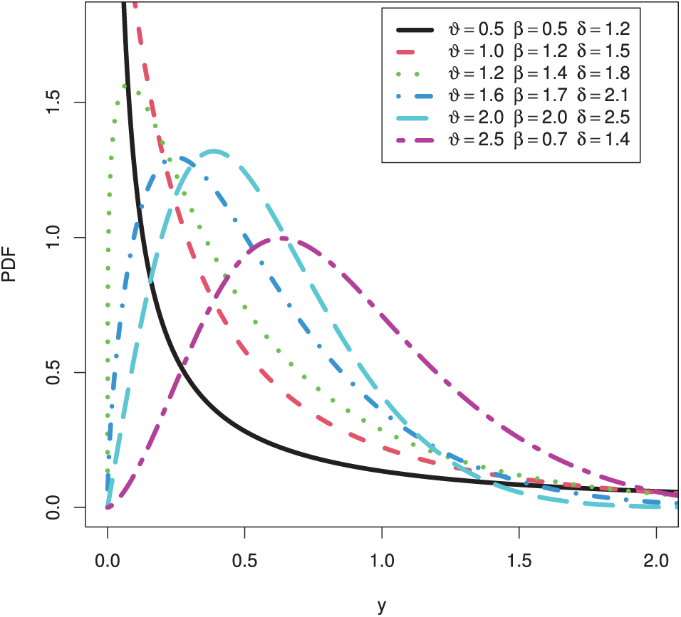
Figure 1: Plots of the PDF for the HTPXLD

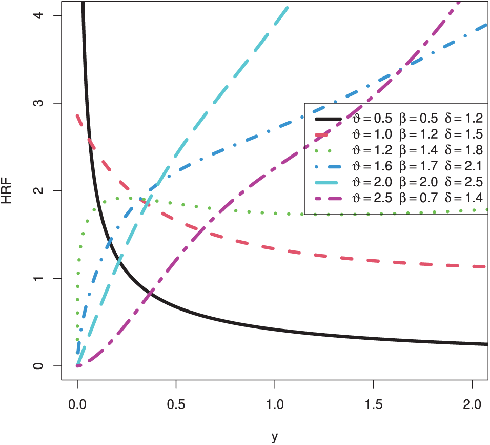
Figure 2: Plots of the HRF for the HTPXLD

3  Statistical Properties

A number of statistical properties, such as QF, moments, IMs, PDF linear expansion, Bonferroni and Lorenz curves, SO, SS parameters, and extropy measures that shed light on the structure of the distribution, will be covered here.

3.1 Series Representation

To analyze most of the statistical properties of HTPXLD, we can express the PDF as a linear combination of simpler functions. Using the following power series:

(7)

in PDF defined in Eq. (6) provides

(8)

Again, using a binomial expansion in PDF (8) yields

(9)

3.2 Quantile Function

In statistical modeling, the QF is essential because it makes it possible to estimate certain percentiles, offers valuable insights into the data distribution, and supports a range of inferential and decision-making procedures. One may determine the QF of the HTPXLD, denoted as , by solving for . Therefore, we must create the following equation:

which leads to

(10)

By multiplying the two sides of Eq. (10) by , one may find the Lambert equation (see [41]), which gives

(11)

Setting to be equal and in Eq. (11) yields the first (), second (), and third () quartiles of the HTPXLD. These quartiles help assess the symmetry (skewness) and peakedness (kurtosis) of the data. Bowley’s skewness () ([42]) and Moor’s kurtosis () ([43]) are statistics calculated using these quartiles to quantify these characteristics precisely. The equations for and are provided below:

and

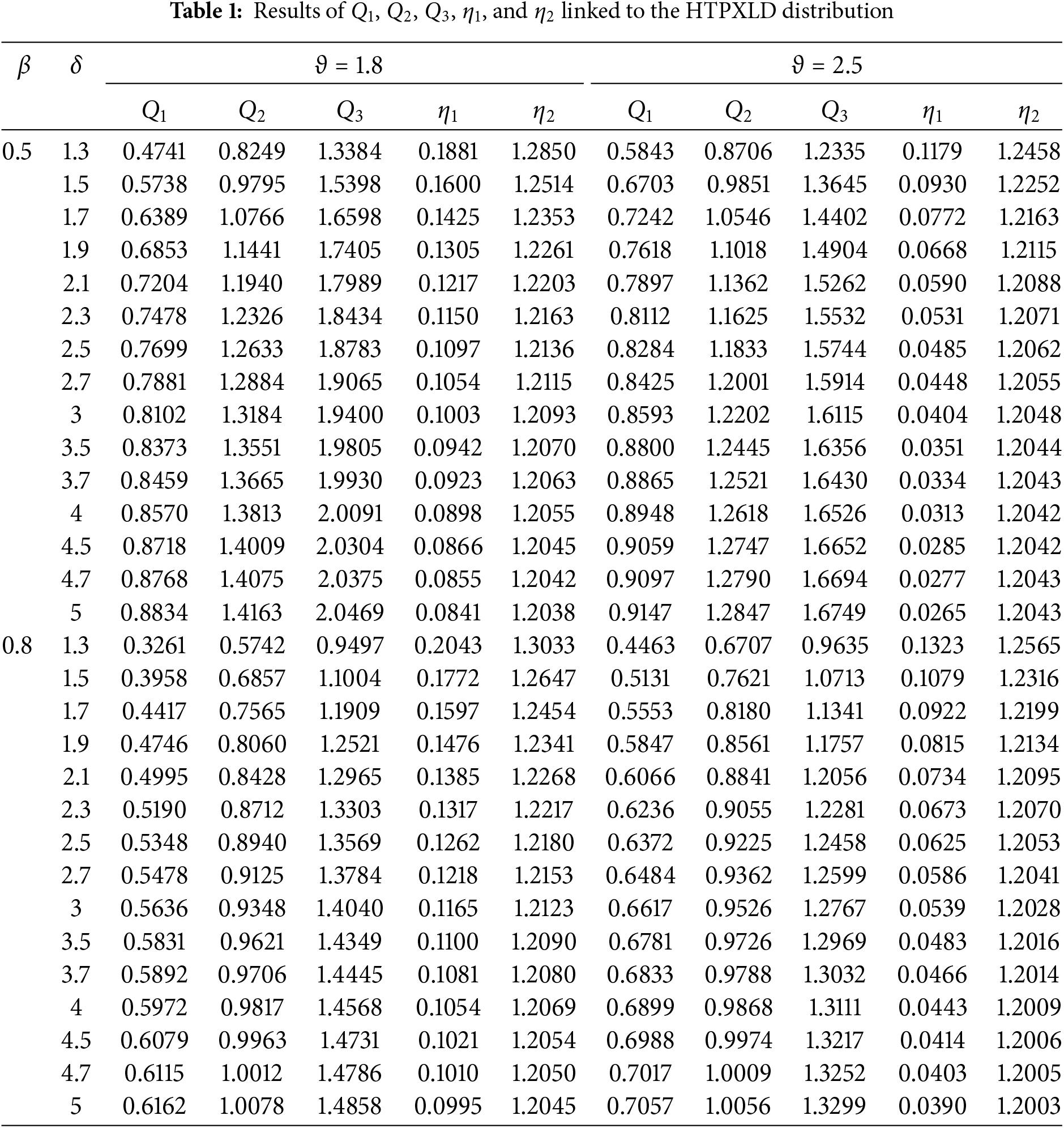
Table 1 presents quantile values (, , ), and of the HTPXLD for various parameter values and values. The table reveals several trends: The data show that increasing leads to higher values for , , and , while and decrease. Values are generally higher at compared to , and there is a consistent trend where , , and increase with , while and decrease.

3.3 Moments

Moments of distribution offer valuable insights into its shape. They reveal measures like central tendency (average), dispersion (spread), skewness (asymmetry), and kurtosis (peakedness). Therefore, deriving the moments is crucial for understanding any new distribution. The k-th moment about the origin of the HTPXLD is obtained by using PDF (9) as follows:

(12)

Using the transformation in (12), we have

(13)

where stands for gamma function (GF). For in (13), the mean of the HTPXLD is produced. Moreover, the k-th central moment of Y may be calculated in the way that follows by utilizing moments around the origin.

Then, using the formulas, and one may find the coefficients of skewness and kurtosis, respectively. They play crucial roles in establishing the asymmetry and flatness of the provided distribution. Also, another important measure is the coefficient of variation (CV), defined by CV , where is the first moment and is the standard deviation.

Likewise, the k-th incomplete moment of the HTPXLD, based on PDF (9), is determined as follows:

(14)

Using the transformation in (14), we have

(15)

where is the lower incomplete GF. One can find applications of incomplete moments by [44].

Tables 2 and 3 present numerical outcomes for the first four moments, variance (), , , and CV for the HTPXLD for some selected parameter values. Based on the positive values of , the HTPXLD exhibits right-skewed. The distribution is characterized as leptokurtic for and platykurtic for .

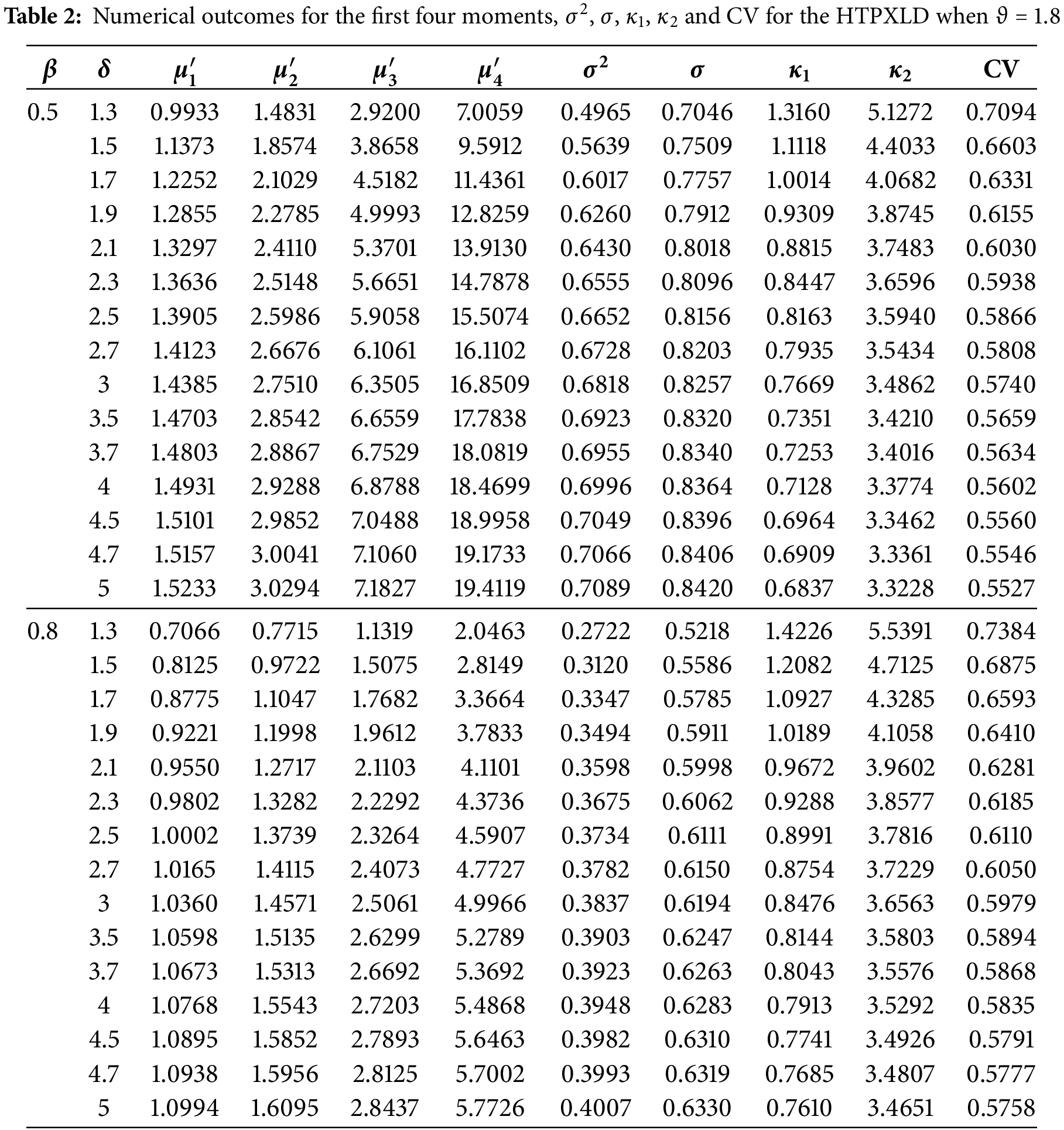
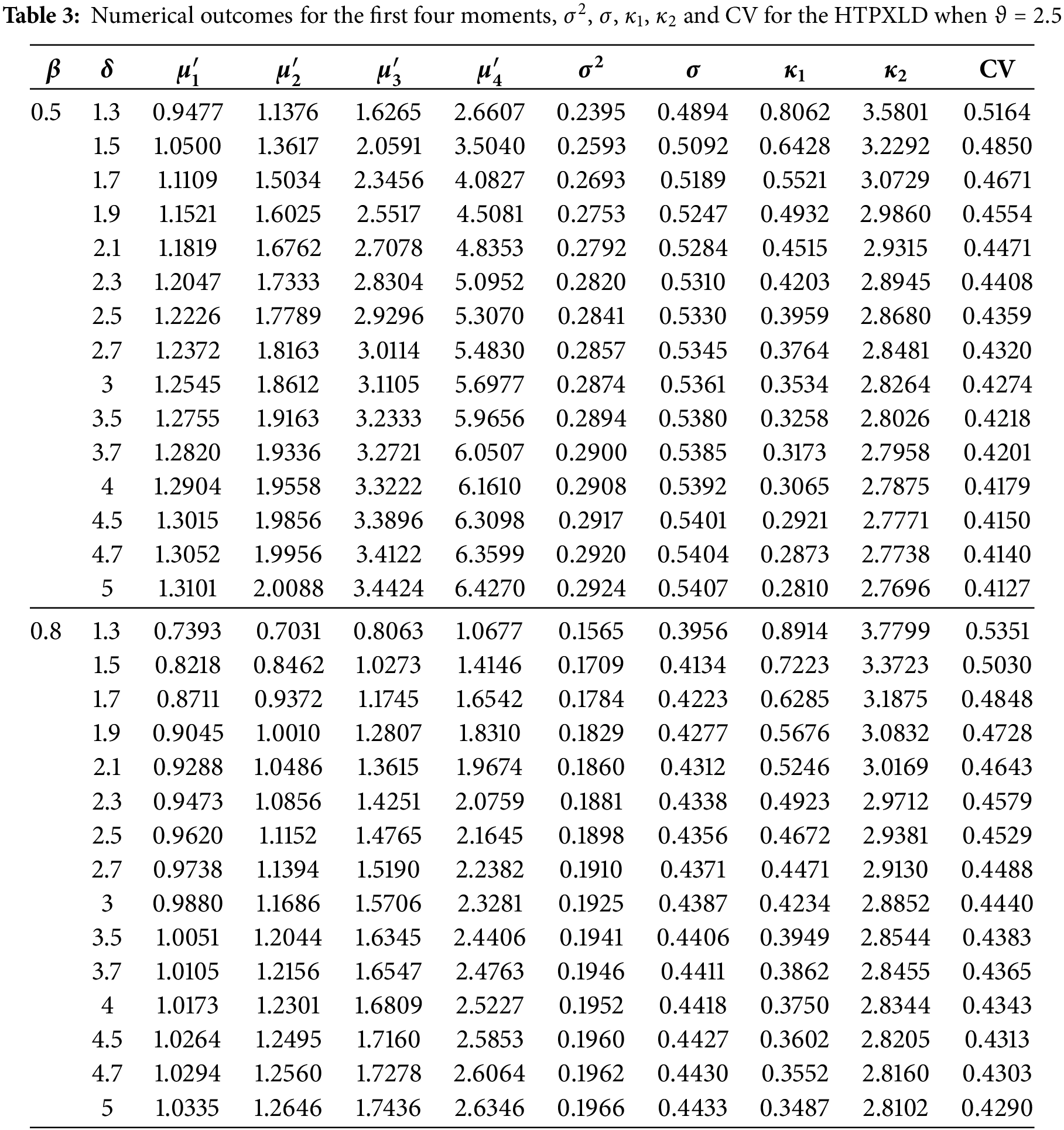
Tables 2 and 3 reveal several trends: As and increase, it shows a decrease in kurtosis, with values in Table 3 being lower than those in Table 2, indicating reduced kurtosis at compared to . The values of , , and CV follow similar trends across the tables, increasing with higher and in both cases.

3.4 Stochastic Ordering

A concept in probability distributions that has been studied in great detail is stochastic ordering, which is crucial for analyzing comparative behavior among random variables in reliability theory and other fields. Stochastic ordering is a powerful tool used in probability and statistics to compare the behavior of random variables. It allows us to understand which random variable is “less risky” or has a “lower probability of taking on extreme values” compared to another. A random variable is regarded as less than a random variable in the following ways:

•   SO (represented by ) if .

•   hazard rate order (represented by ) if .

•   likelihood ratio order (represented by ) if decreases in .

According to Shaked et al. [45], the following impacts are widely recognized:

Let HTPXLD , and HTPXLD , , then the likelihood ratio ordering is as follows:

then

For we get for all hence is decreasing in and hence .

3.5 Extropy Measures

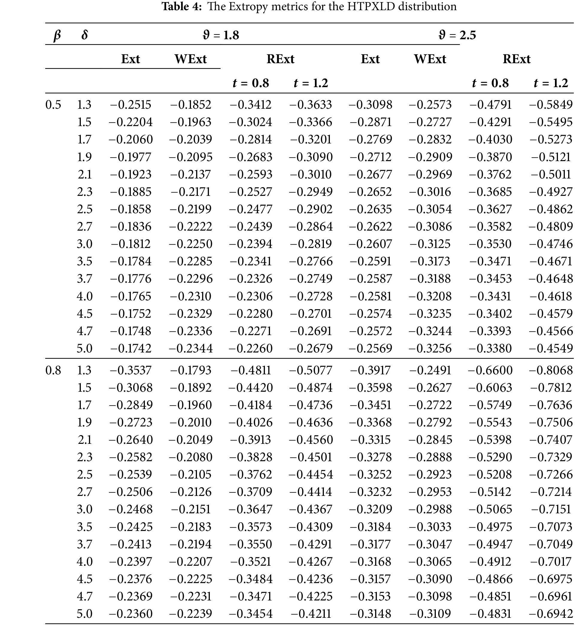
The extropy (Ext), which is the double complement of the entropy [46], was developed as an alternative uncertainty measure by Lad et al. [47]. The Ext can be statistically utilized to evaluate the accuracy of predicted distributions through the total log scoring method. For a non-negative random variableY, Ext is defined as follows:

(16)

Thus, using PDF (6) in (16), the extropy of the HTPXLD may be represented as follows:

(17)

Using the expansion (7) in (17) gives

(18)

Using binomial expansion in (18), we have

Then after some simplified form, the previous equation will be

(19)

Using the transformation in (19), the extropy measure of HTPXLD thus has the following structure after some simplification:

where

Weighted extropy (WExt), introduced by [48], offers an alternative perspective to traditional entropy. Unlike entropy, it assigns greater weight to larger values within a probability distribution. It can be expressed, mathematically, by

(20)

Then by inserting PDF (6) in (20), then the WExt is

Using the similar procedure discussed above, then is as follows:

The residual extropy (RExt) at the time of residual lifespan is given by

(21)

Then, by inserting PDF (6) in (21) and using the similar procedure discussed above, the RExt will be

where is the upper incomplete GF. According to Table 4, for both values of , there is a discernible trend in the Ext and RExt measures towards becoming less negative with rising . Both Ext and RExt exhibit a decline in negativity as rises. On the other hand, WExt’s negativity steadily drops as rises. When is used instead of , the decline in WExt is more gradual and more noticeable at higher values.

3.6 Stress-Strength Model

The SS model is a powerful tool in reliability engineering used to assess the probability of a component surviving under operational conditions. It considers two random variables: strength (X), which stands for the component’s intrinsic ability to withstand stress (Y). Therefore, the core concept of the SS model is captured by the following equation: , where R represents the reliability, or the probability of the component functioning successfully. This model has a wide range of applications across various scientific fields. Let the strength X HTPXLD and stress Y HTPXLD then the SS parameter for the HTPXLD is given by

(22)

where and Using expansion (7) twice for the numerator of Eq. (22) gives

(23)

(24)

After simplifying Eq. (24), we get

(25)

where and

Note that the integrals in Eq. (25) can be obtained as follows:

Then, by inserting and , in the Eq. (25), the SS parameter of HTPXLD is as follows:

4  Actuarial Measures

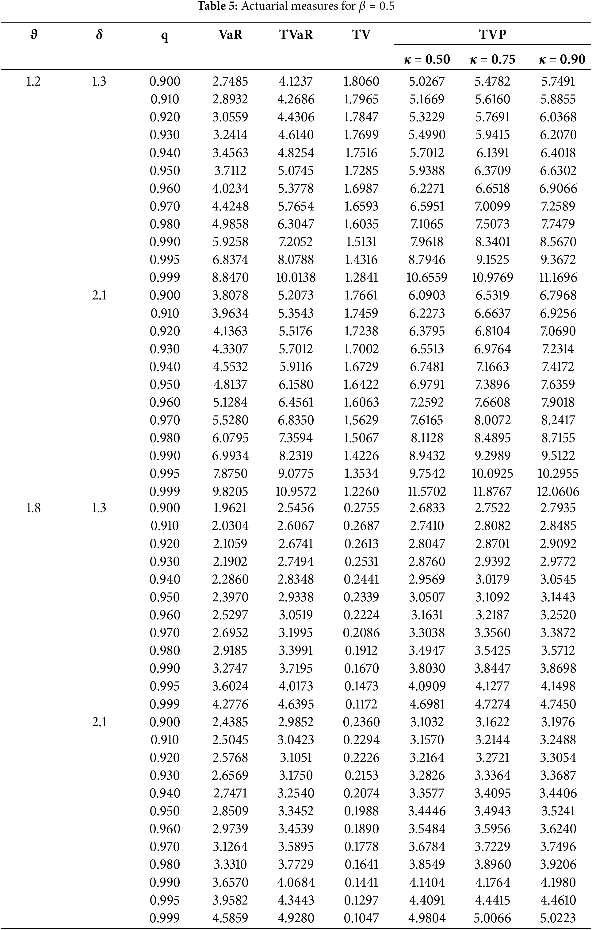
This section introduces several well-known risk measures for the developed model. These measures include Value-at-Risk (VaR), Tail Value-at-Risk (TVaR), Tail Variance (TV), and Tail Variance Premium (TVP).

4.1 Value-at-Risk

As outlined in reference [49], the quantile of a random variable’s CDF corresponds to its VaR. The VaR for the HTPXLD is given by

(26)

4.2 Tail Value-at-Risk

TVaR is a crucial risk measure that evaluates the expected loss beyond a specified probability level, once an event has occurred. For the HTPXLD, the TVaR is defined as

4.3 Tail Variance and Tail Variance Premium

Landsman [50] first introduced the TV risk measure, which is defined by the variance of the loss distribution above a certain critical threshold. The TV for the HTPXLD can be expressed as

4.4 Tail Variance Premium

The TVP combines statistics related to both the central tendency and dispersion of the data, making it a significant risk measure. The TVP for the HTPXLD is given by

Table 5 demonstrates several key trends: Increasing values lead to higher VaR and TVaR values, indicating an overall increase in risk measures. For example, higher values correspond to higher risk estimates. For a given , higher results in greater TVP values across all levels. This indicates a more pronounced sensitivity to risk with increasing . Within the same and settings, TVP values rise with , reflecting a higher quantile level and, consequently, increased risk assessment.

5  Parameter Estimation

Our main goal in this section is to use the ML estimation method to obtain the point and interval estimates of the unknown parameters of the HTPXLD. Assume that , a sample of size , is taken from the HTPXLD specified by the PDF (6). For the vector of parameters the log-likelihood function can be written as

Regarding the model parameters and the partial derivatives of are obtained, respectively, as follows:

(27)

(28)

(29)

The non-linear Eqs. (27)–(29) are equated with zero to obtain the ML estimates (MLEs) and As seen, it is difficult to formulate easily, making it challenging to solve them directly for the vector parameter Consequently, iterative techniques are used, such as the Newton-Raphson to get MLEs and

Instead of determining point estimates for the unknown parameters, it would be more helpful to identify a range of values that, with a specified probability, encompass them. These ranges are referred to as interval estimates. To build the parameters CIs, the asymptotic distribution of MLE of will be used, that is

where is the MLE of and is the inverse of the observed information matrix of , and it is given by

Asymptotic normality of the MLEs allows for the construction of the asymptotic CIs of and for and respectively.

where is the upper th percentile point of the standard normal distribution.

6  Simulation

This section presents a simulation study to assess the performance of MLEs for the HTPXLD parameters . The R package is utilized to compute the mean, relative bias (RBias), bias, mean squared error (MSE), root mean squared error (RMSE), average interval length (AIL) of 95%, and coverage probability (CP) of 95% for the estimated values of , , and . The simulation process is outlined as follows:

1)   Generate 5000 random samples from the HTPXLD with sizes = 50, 100, 150, 200, 250, 300, 350, and 400.

2)   Choose parameter values for the simulations as follows: set1 = ( = 0.8, = 1.5, = 0.7), set2 = ( = 0.5, = 1.5, = 0.7), set3 = ( = 0.5, = 1.2, = 0.3), set4 = ( = 0.7, = 1.6, = 0.4), set5 = ( = 1.1, = 1.9, = 0.7), and set6 = ( = 0.4, = 1.7, = 0.9).

3)   Compute the MLEs, RBiases, Biases, RMSEs, and MSEs for each sample size and parameter set. Additionally, calculate the AIL and CP at a 95% confidence level for all sample sizes and parameter sets.

4)   Present the numerical results in Tables 6–8. The performance of the estimated parameters is analyzed based on complete samples.

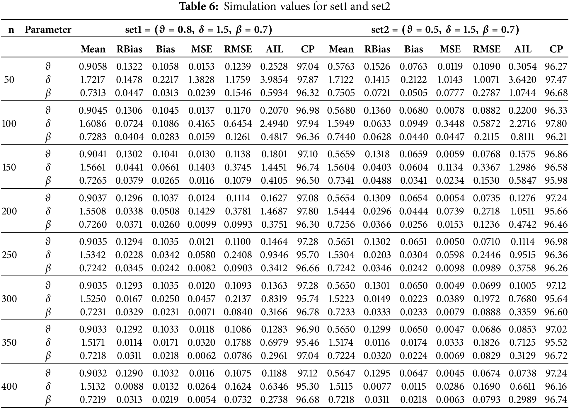
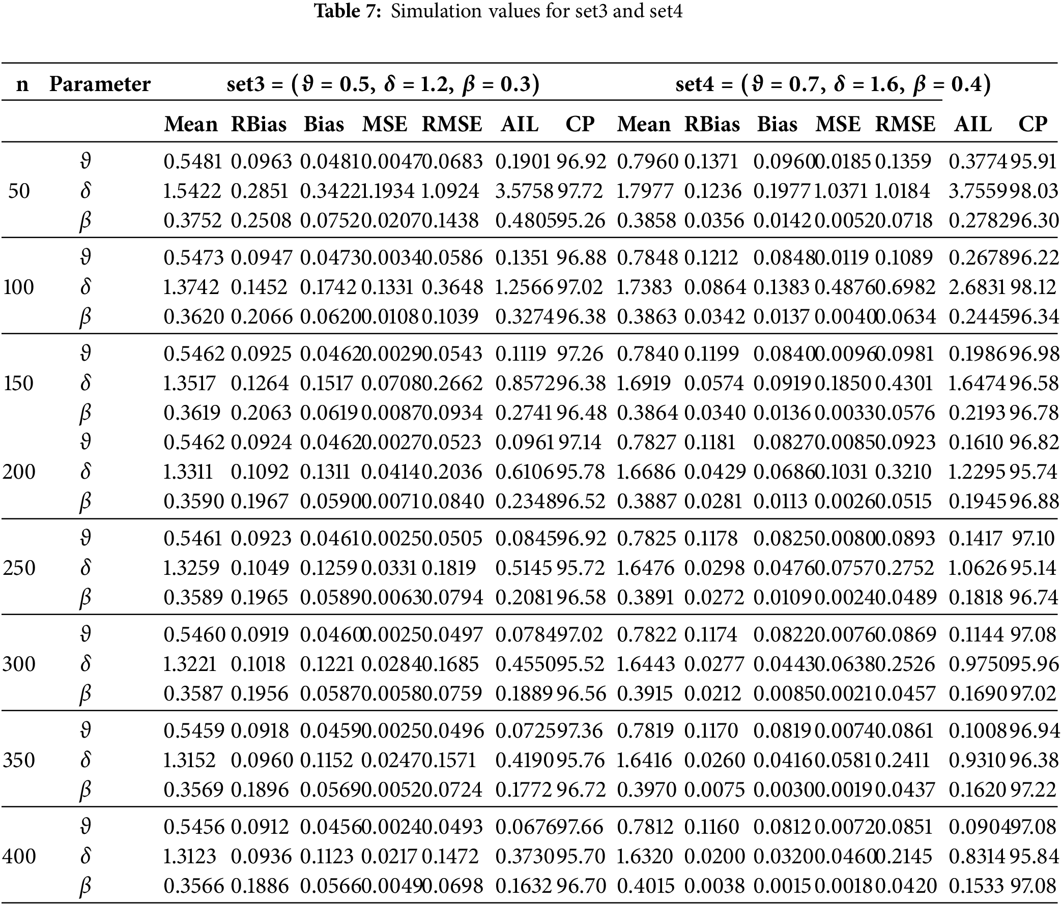
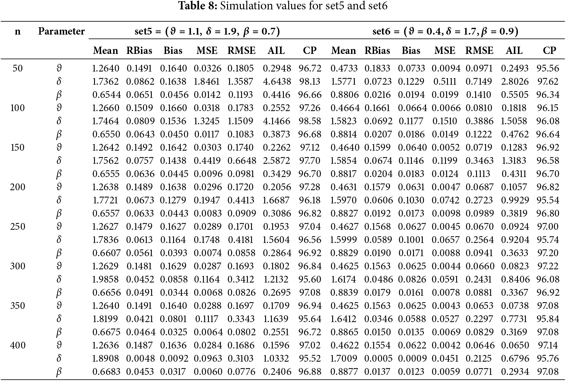
The results show in Tables 6–8 that bias, MSE, and RMSE all significantly decrease with increasing sample size (n). Furthermore, higher sample sizes increase CP and AIL, producing more accurate and trustworthy estimates and confidence ranges.

•   Greater sample sizes lead to improvements in MSE. As the sample size increases, the parameter estimates converge closer to the real values, indicating that the MLEs are becoming more exact, as indicated by lower MSE values.

•   As the sample size grows, the CP gets better, indicating that the CIs created for the parameter estimates get more trustworthy. The robustness of the estimates is improved by higher CP values, which indicate a higher probability that the intervals include the genuine parameter values.

•   As the sample size grows, the values of AIL become lower.

7  Applications

This section demonstrates the applicability of the HTPXLD in fitting real-world data by evaluating it against three actual datasets. The HTPXLD is compared with several alternative models, including XLD [1], Lindley (LD) [51], exponentiated generalized XLD (EGXLD) [52], power exponentiated LD (PELD) [53], Kumaraswamy LD (KLD) [54], Weibull power LD (WPLD) [15], exponentiated generalized power LD (EGLD) [55], power LD (PLD) [56], Weibull LD (WLD) [57], extended LD (EXLD) [58], and PXLD.

We use nine well-established goodness-of-fit measures to compare these models, including the Kolmogorov-Smirnov () statistic, its p-value (), Anderson-Darling statistics (), its p-value (), the Hannan-Quinn Information Criterion (), Akaike Information Criterion (), Bayesian Information Criterion (), Consistent (), Cramér-von Mises statistic (), and its p-value (). The optimal model is identified based on the highest values for , , and , and the lowest values for , , , , , , and .

7.1 The First Dataset

The first dataset consists of repair times for an airborne communication transceiver, provided by [59]. The recorded times are: 0.50, 0.60, 0.60, 0.70, 0.70, 0.70, 0.80, 0.80, 1.00, 1.00, 1.00, 1.00, 1.10, 1.30, 1.50, 1.50, 1.50, 1.50, 2.00, 2.00, 2.20, 2.50, 2.70, 3.00, 3.00, 3.30, 4.00, 4.00, 4.50, 4.70, 5.00, 5.40, 5.40, 7.00, 7.50, 8.80, 9.00, 10.20, 22.00, 24.50. Table 9 displays the results of the descriptive analysis for this dataset.

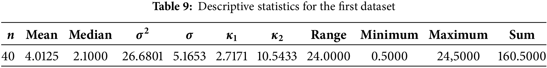
For the first dataset, Table 10 presents the MLEs along with their standard errors (SEs). Table 11 provides the numerical values for the statistic, its , , its , , its , as well as the , , , and statistics. Fig. 3 includes the histogram, violin plot, QQ (quantile-quantile) plot, box plot with strip chart, and TTT (total time in test) plot. The estimated PDFs of competing models for the first dataset are shown in Fig. 4, while Fig. 5 displays the estimated CDFs of the competitive models. Additionally, Fig. 6 illustrates the PP plots of the competing models. Figs. 4–6 demonstrate the fit of our distribution to the actual data.

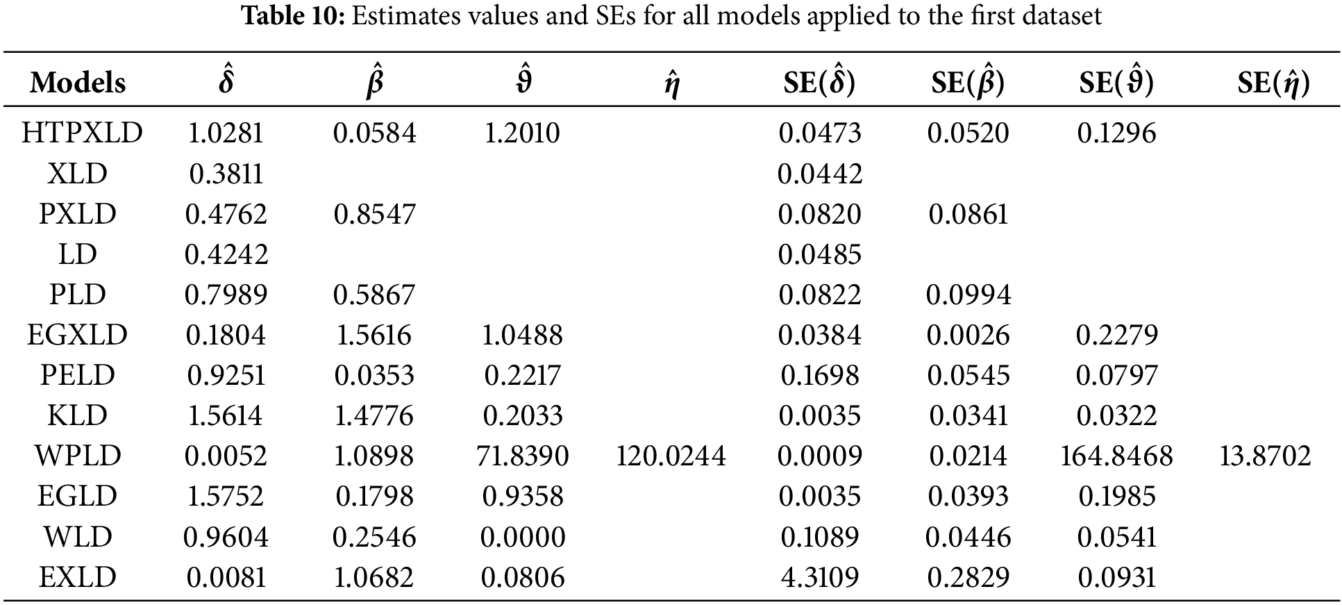
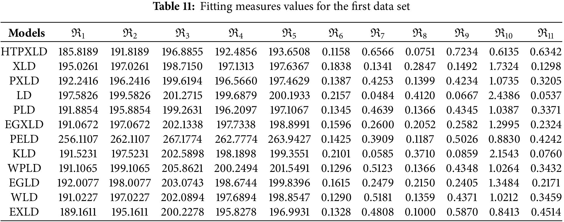
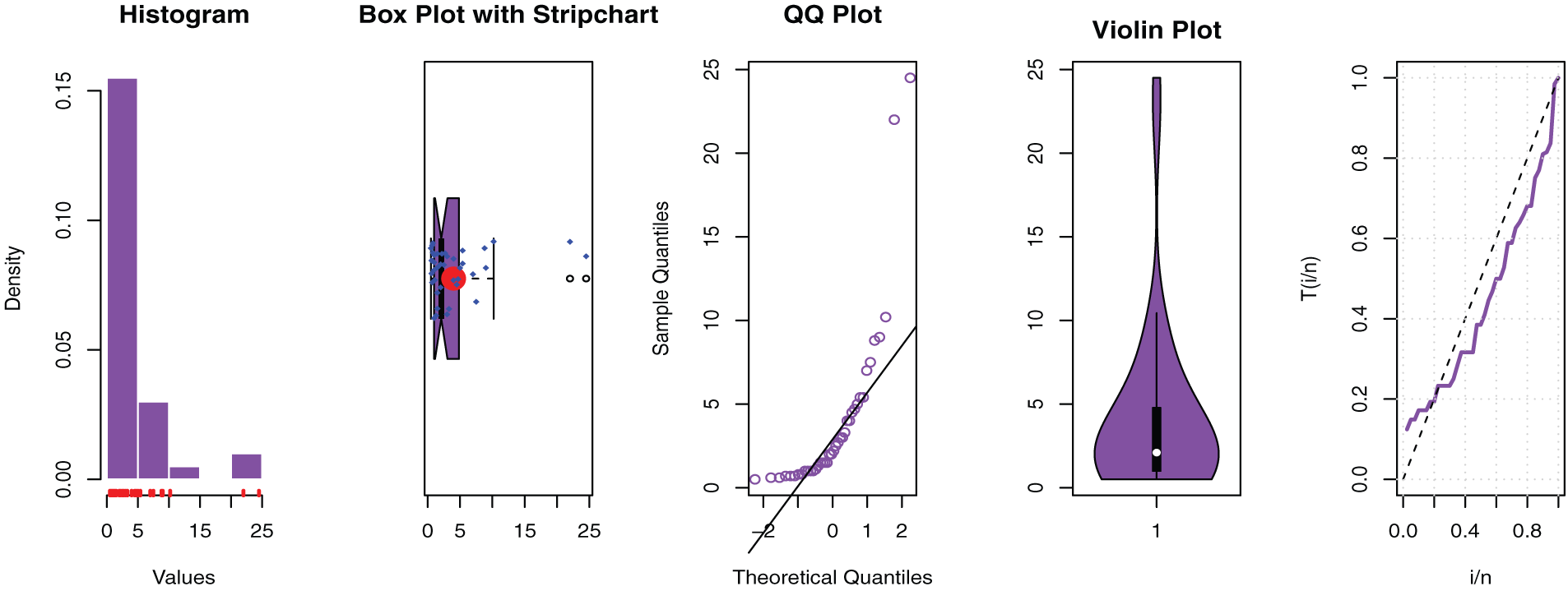
Figure 3: Some basic non-parametric plots for the first dataset

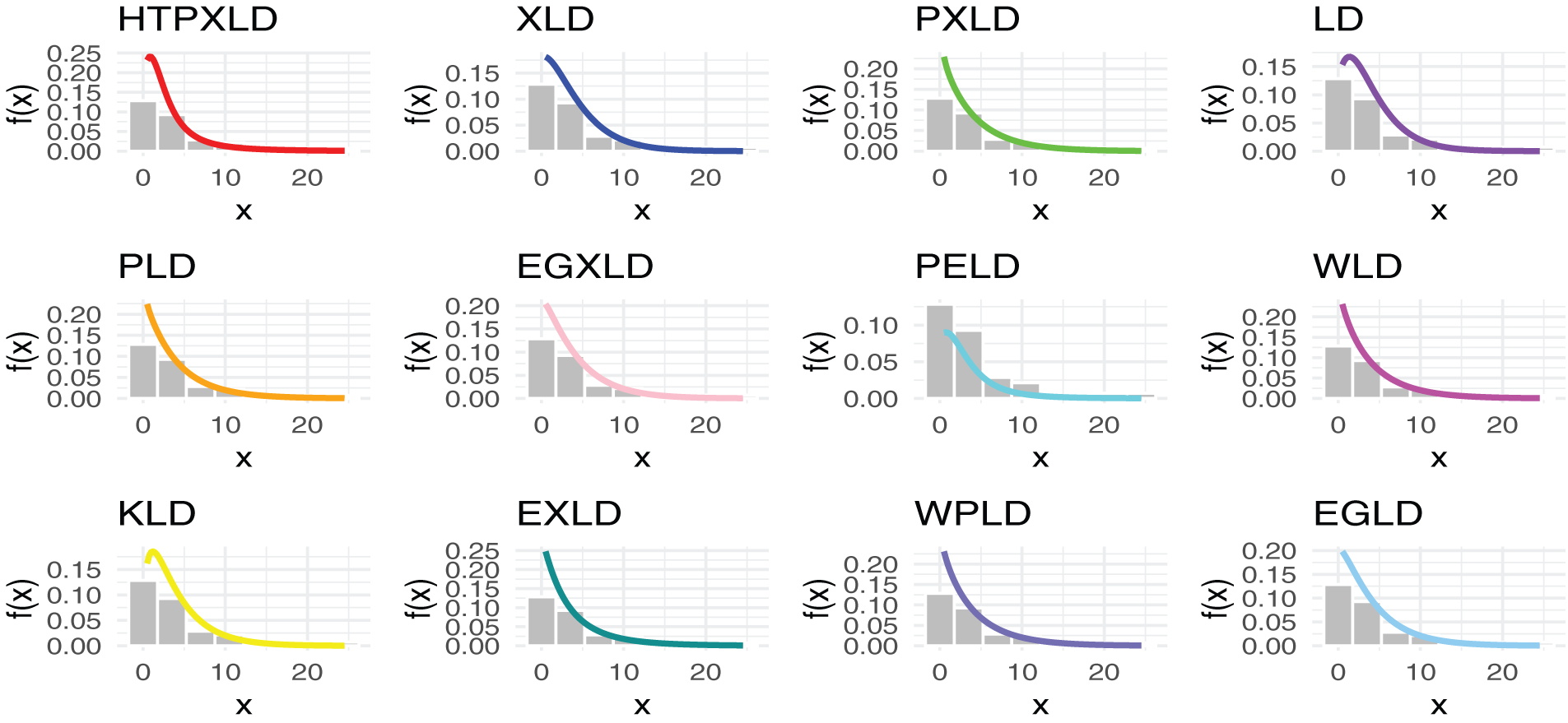
Figure 4: Estimated PDFs for the competing models for the first dataset

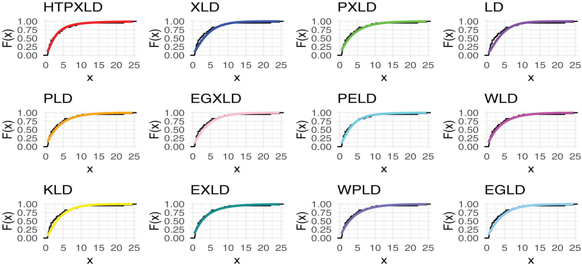
Figure 5: Estimated CDFs for the competing models for the first dataset

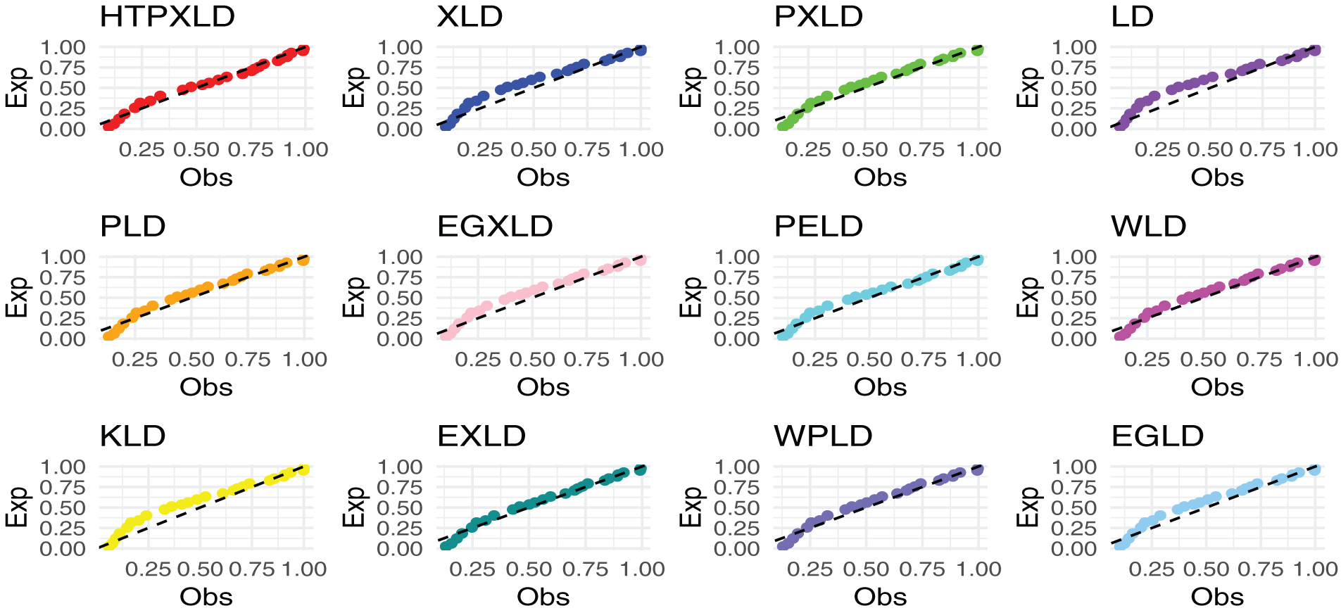
Figure 6: PP plots of competing models for the first dataset

7.2 The Second Dataset

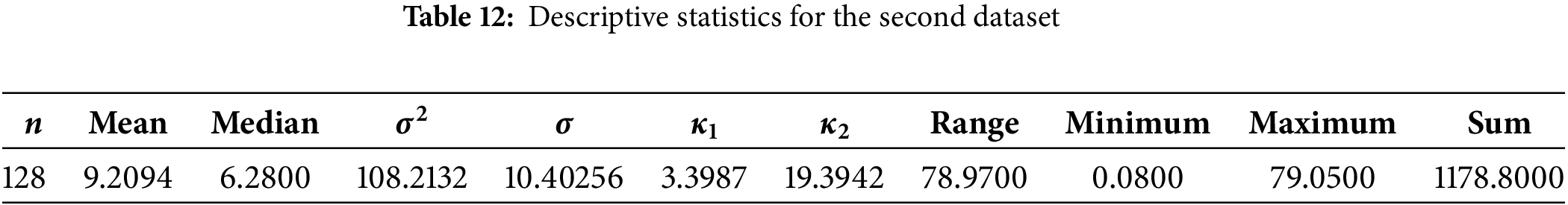
The data set provided by [60] shows the monthly remission periods of 128 individuals with bladder cancer who were selected at random. the data set that we work with is 0.08, 2.09, 3.48, 4.87, 6.94, 8.66, 13.11, 23.63, 0.2, 2.23, 3.52, 4.98, 6.97, 9.02, 13.29, 0.4, 2.26, 3.57, 5.06, 7.09, 9.22, 13.8, 25.74, 0.5, 2.46, 3.64, 5.09, 7.26, 9.47, 14.24, 25.82, 0.51, 2.54, 3.7, 5.17, 7.28, 9.74, 14.76, 6.31, 0.81, 2.62, 3.82, 5.32, 7.32, 10.06, 14.77, 32.15, 2.64, 3.88, 5.32, 7.39, 10.34, 14.83, 34.26, 0.9, 2.69, 4.18, 5.34, 7.59, 10.66, 15.96, 36.66, 1.05, 2.69, 4.23, 5.41, 7.62, 10.75, 16.62, 43.01, 1.19, 2.75, 4.26, 5.41, 7.63, 17.12, 46.12, 1.26, 2.83, 4.33, 5.49, 7.66, 11.25, 17.14, 79.05, 1.35, 2.87, 5.62, 7.87, 11.64, 17.36, 1.4, 3.02, 4.34, 5.71, 7.93, 11.79, 18.1, 1.46, 4.4, 5.85, 8.26, 11.98, 19.13, 1.76, 3.25, 4.5, 6.25, 8.37, 12.02, 2.02, 3.31, 4.51, 6.54, 8.53, 12.03, 20.28, 2.02, 3.36, 6.76, 12.07, 21.73, 2.07, 3.36, 6.93, 8.65, 12.63, 22.69.

Table 12 displays the results of the descriptive analysis for this dataset.

For the second dataset, Table 13 presents the MLEs along with their SEs. Table 14 provides the numerical values for the statistic, its , , its , , its , as well as the , , , and statistics. Fig. 7 includes the histogram, violin plot, QQ plot, box plot with strip chart, and TTT plot. The estimated PDFs of competing models for the second dataset are shown in Fig. 8, while Fig. 9 displays the estimated CDFs of the competitive models. Additionally, Fig. 10 illustrates the PP plots of the competing models. Figs. 8–10 demonstrated the fit of our distribution to the actual data.

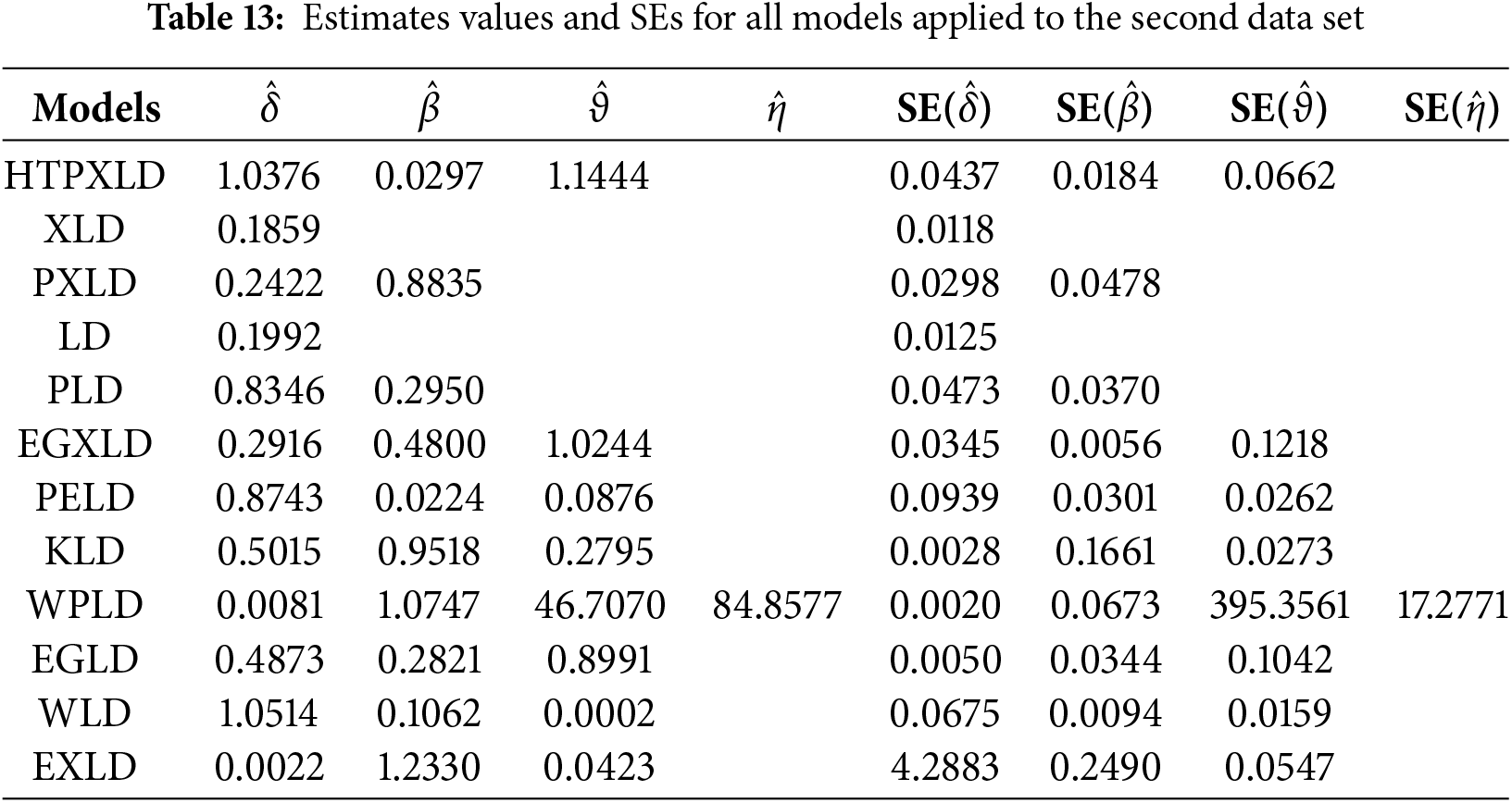
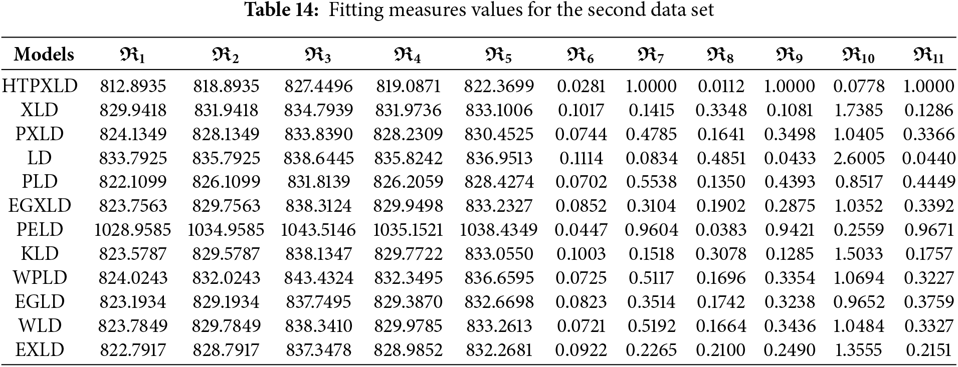
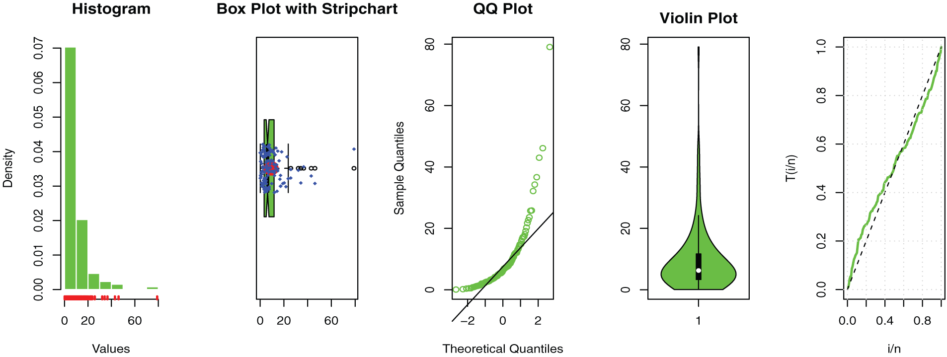
Figure 7: Some basic non-parametric plots for the second dataset

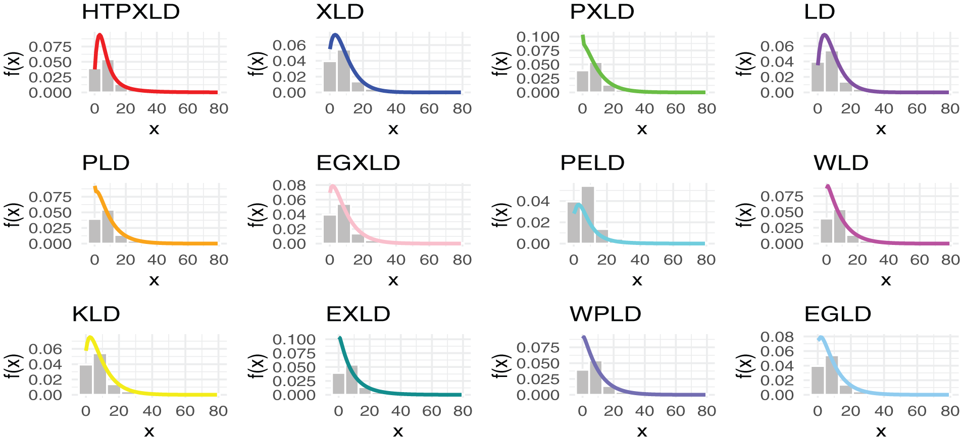
Figure 8: Estimated PDFs for the competing models for the second dataset

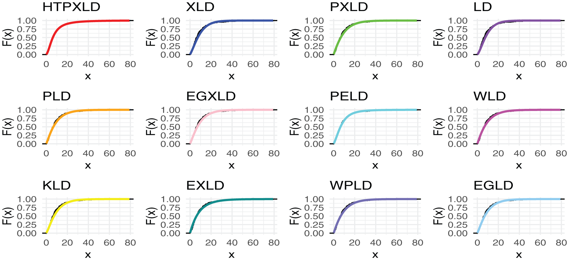
Figure 9: Estimated CDFs for the competing models for the second dataset

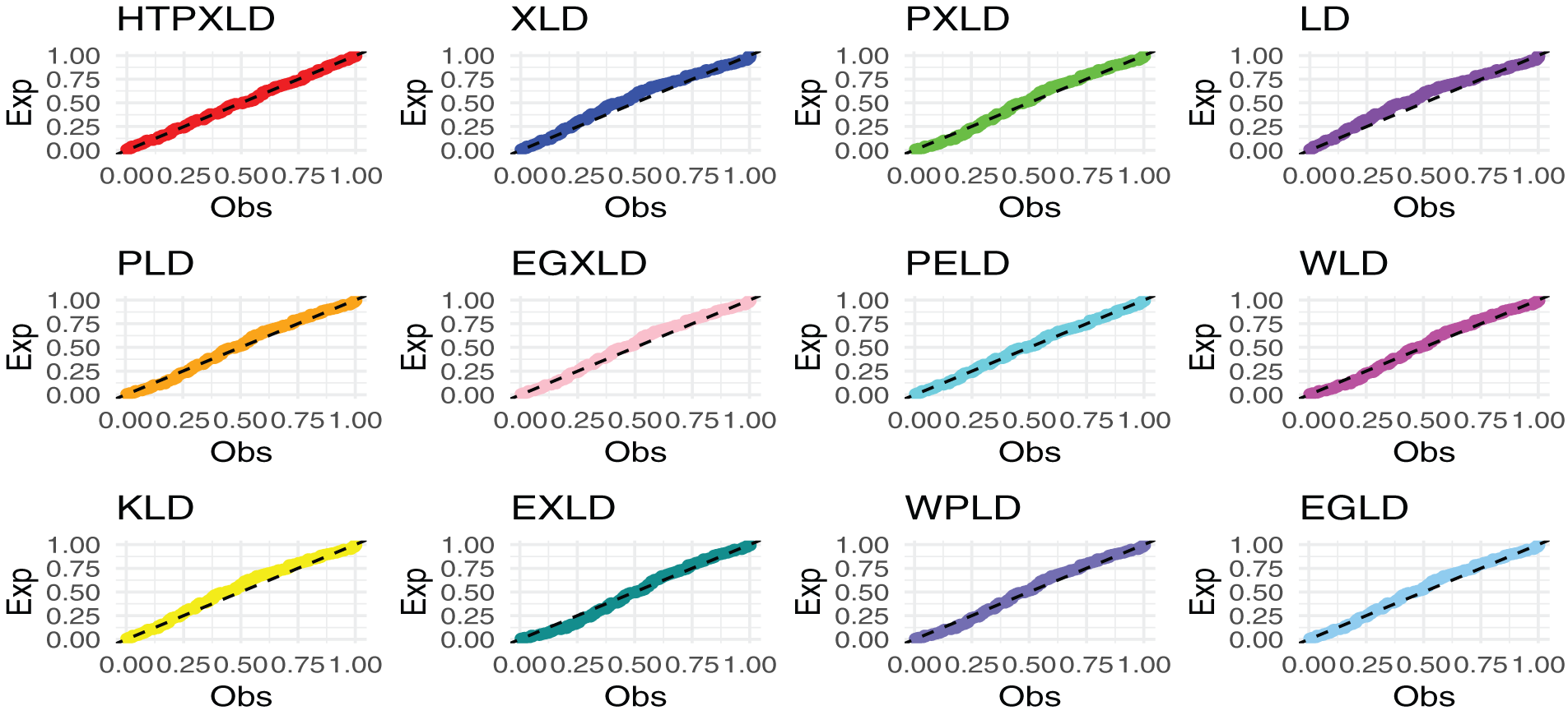
Figure 10: Estimated CDFs for the competing models for the second dataset

7.3 The Third Dataset

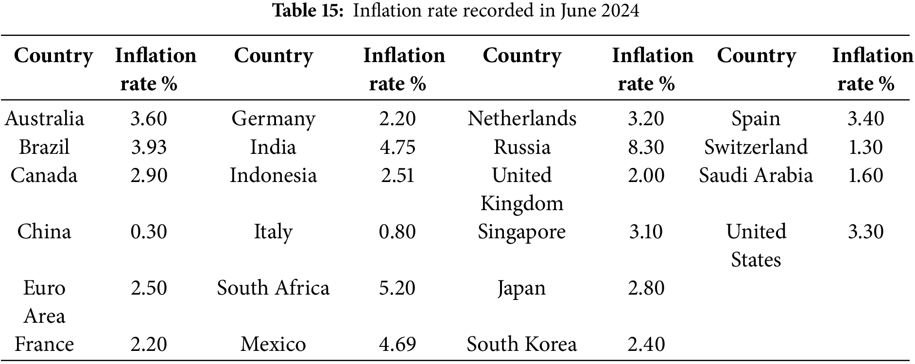
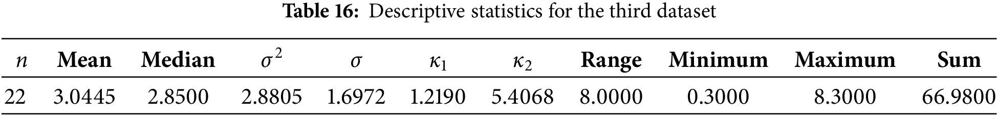
The third data set represents values for the inflation rate in several countries that were recorded in June 2024. The term “inflation rate” describes how prices for products and services vary over time. The electronic address from which it was taken is as follows: https://tradingeconomics.com/ (accessed on 07 February 2025). The data set is reported in Table 15. Table 16 displays the results of the descriptive analysis for this dataset.

For the third dataset, Table 17 presents the MLEs along with their SEs. Table 18 provides the numerical values for the statistic, its , , its , , its , as well as the , , , and statistics. Fig. 11 includes the histogram, violin plot, QQ plot, box plot with strip chart, and TTT plot. The estimated PDFs of competing models for the third dataset are shown in Fig. 12, while Fig. 13 displays the estimated CDFs of the competitive models. Additionally, Fig. 14 illustrates the PP plots of the competing models. Figs. 12–14 demonstrate the fit of our distribution to the actual data.

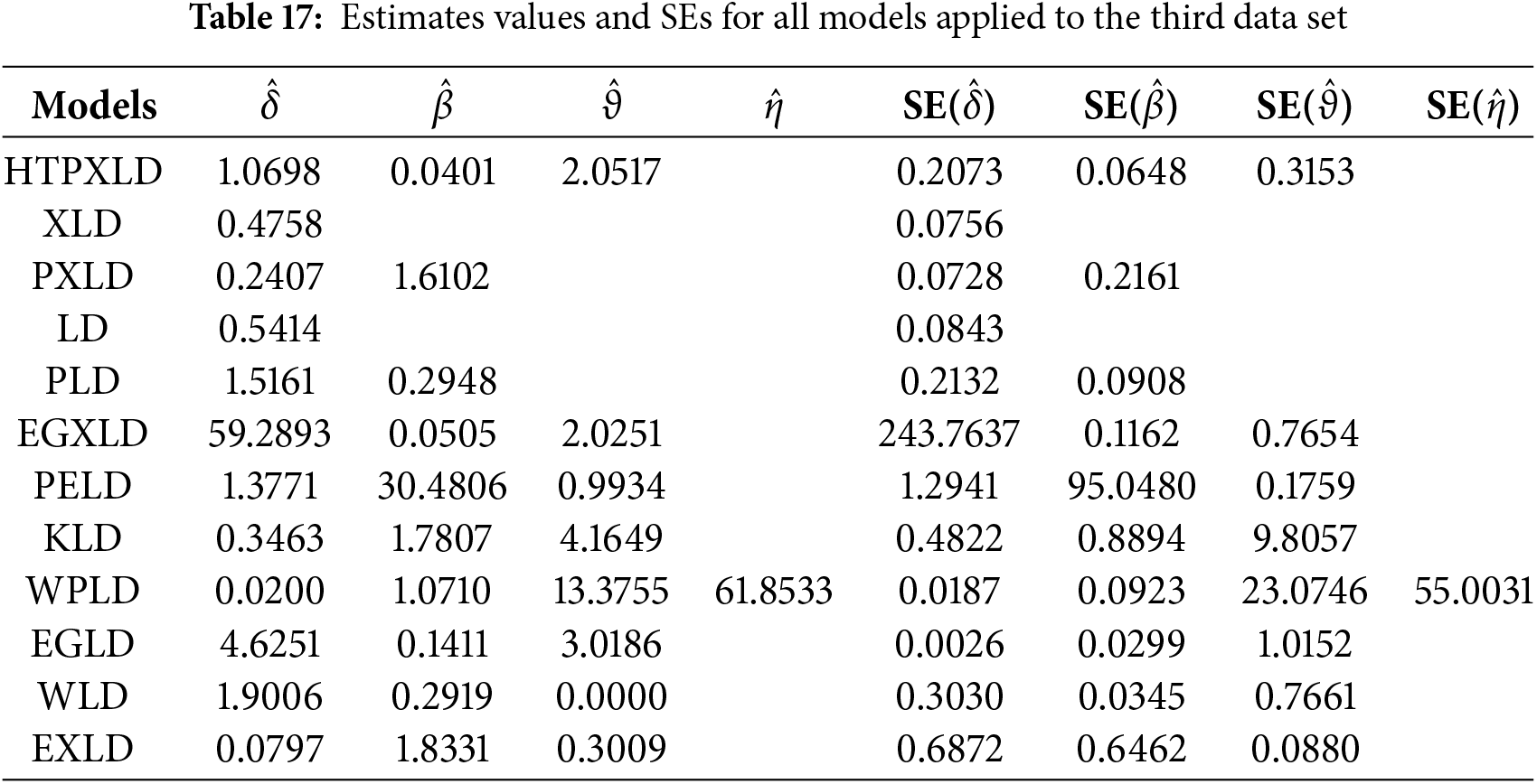
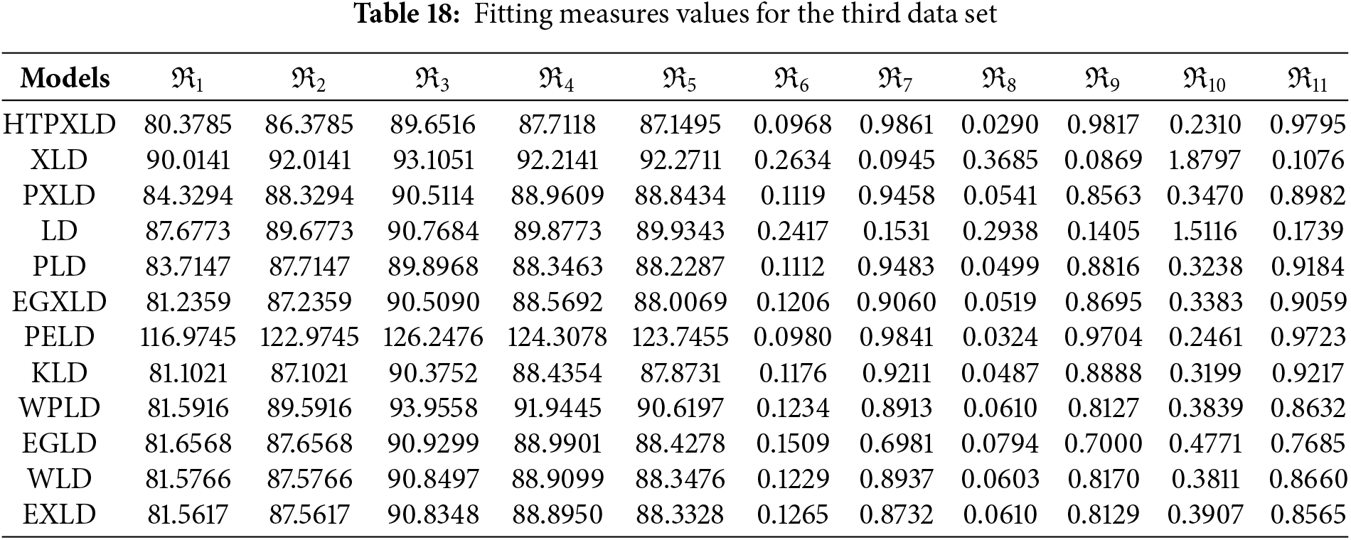
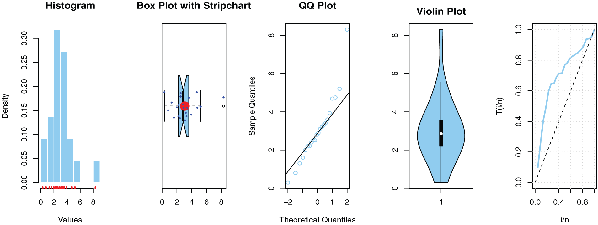
Figure 11: Some basic non-parametric plots for the third dataset

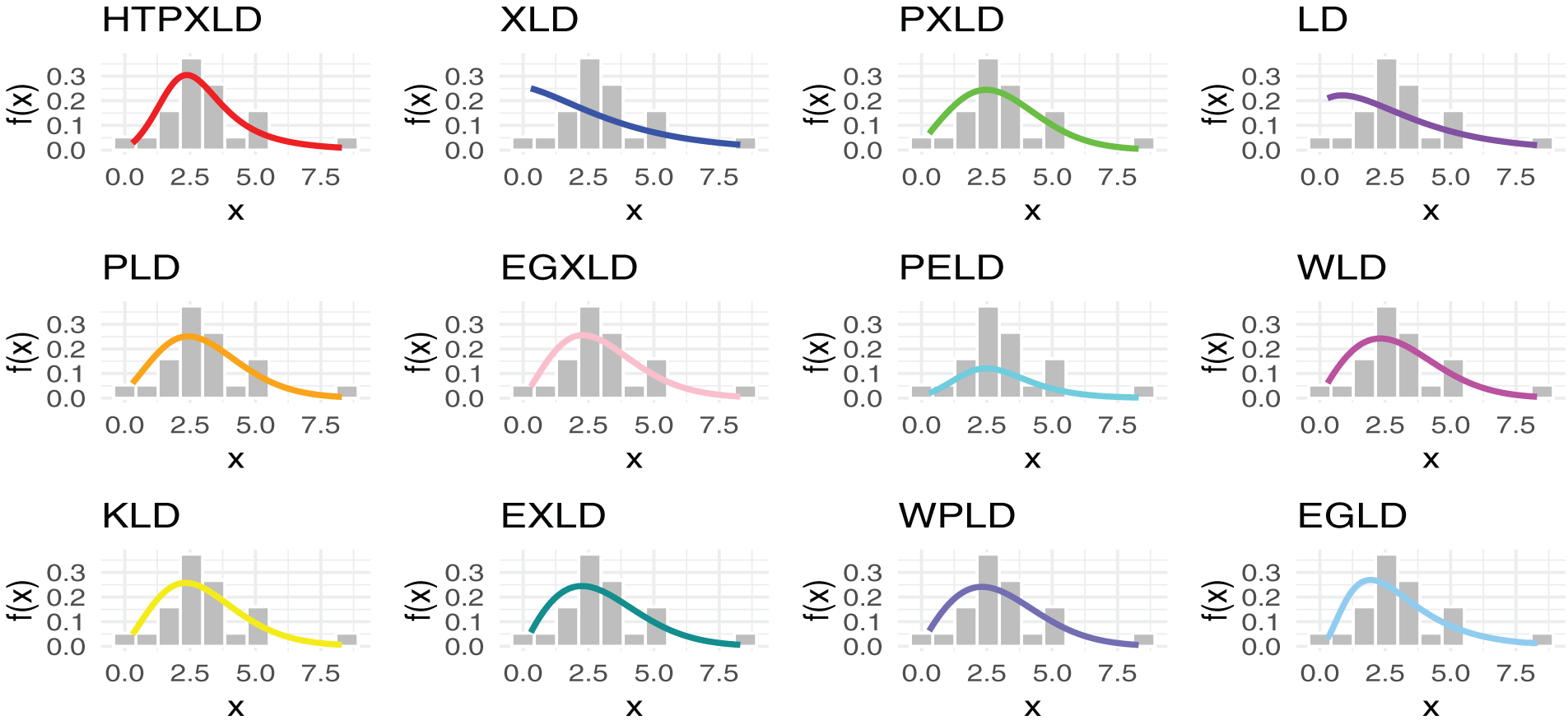
Figure 12: Estimated PDFs for the competing models for the third dataset

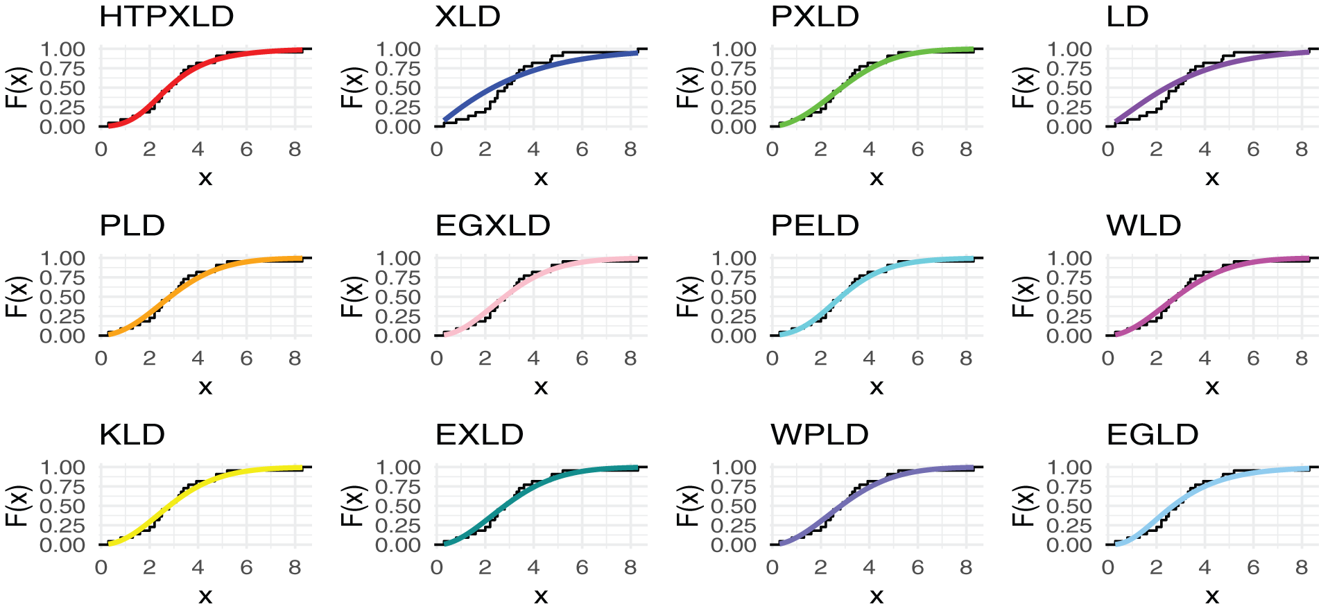
Figure 13: Estimated CDFs for the competing models for the third dataset

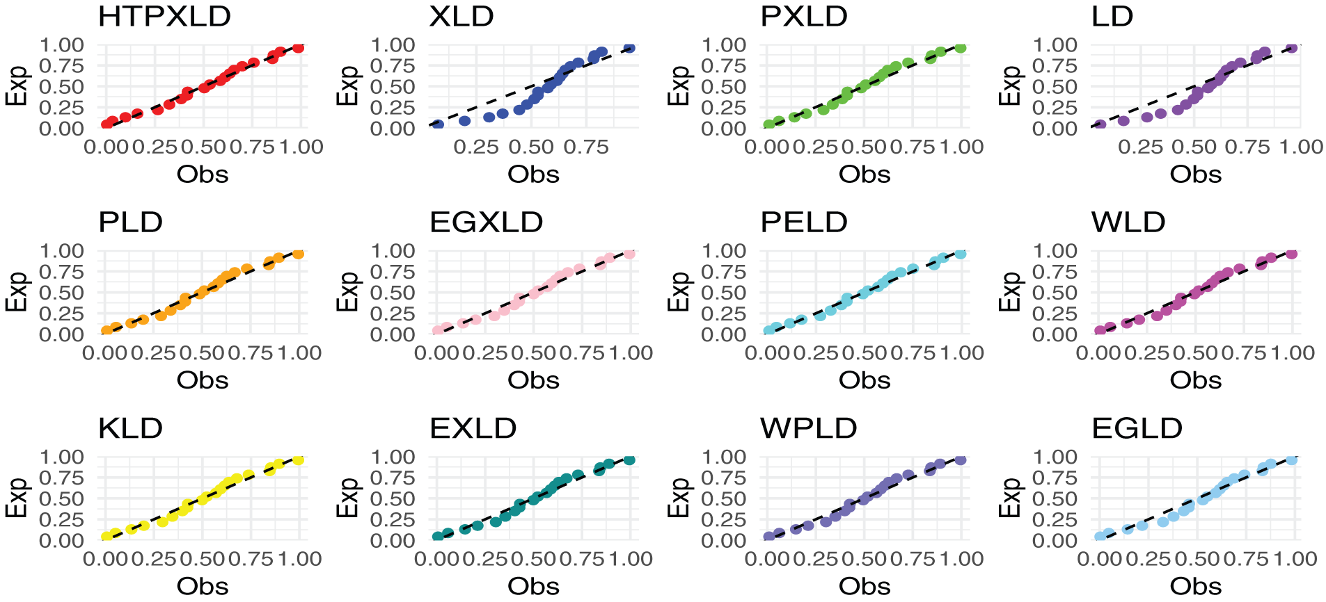
Figure 14: PP plots of competing models for the third dataset

From the numerical values in Tables 11, 14, and 18 the HTPXLD is better than XLD, LD, EGXLD, PELD, KLD, WPLD, EGLD, PLD, WLD, EXLD, and PXLD for the three datasets.

The actuarial measures VaR, TVaR, TV, and TVP of the HTPXLD, PXLD, PLD, EGXLD, WLD, KLD, EXLD, and WPLD are computed and compared using the third data set in the following. Tables 19 and 20 present the numerical findings.

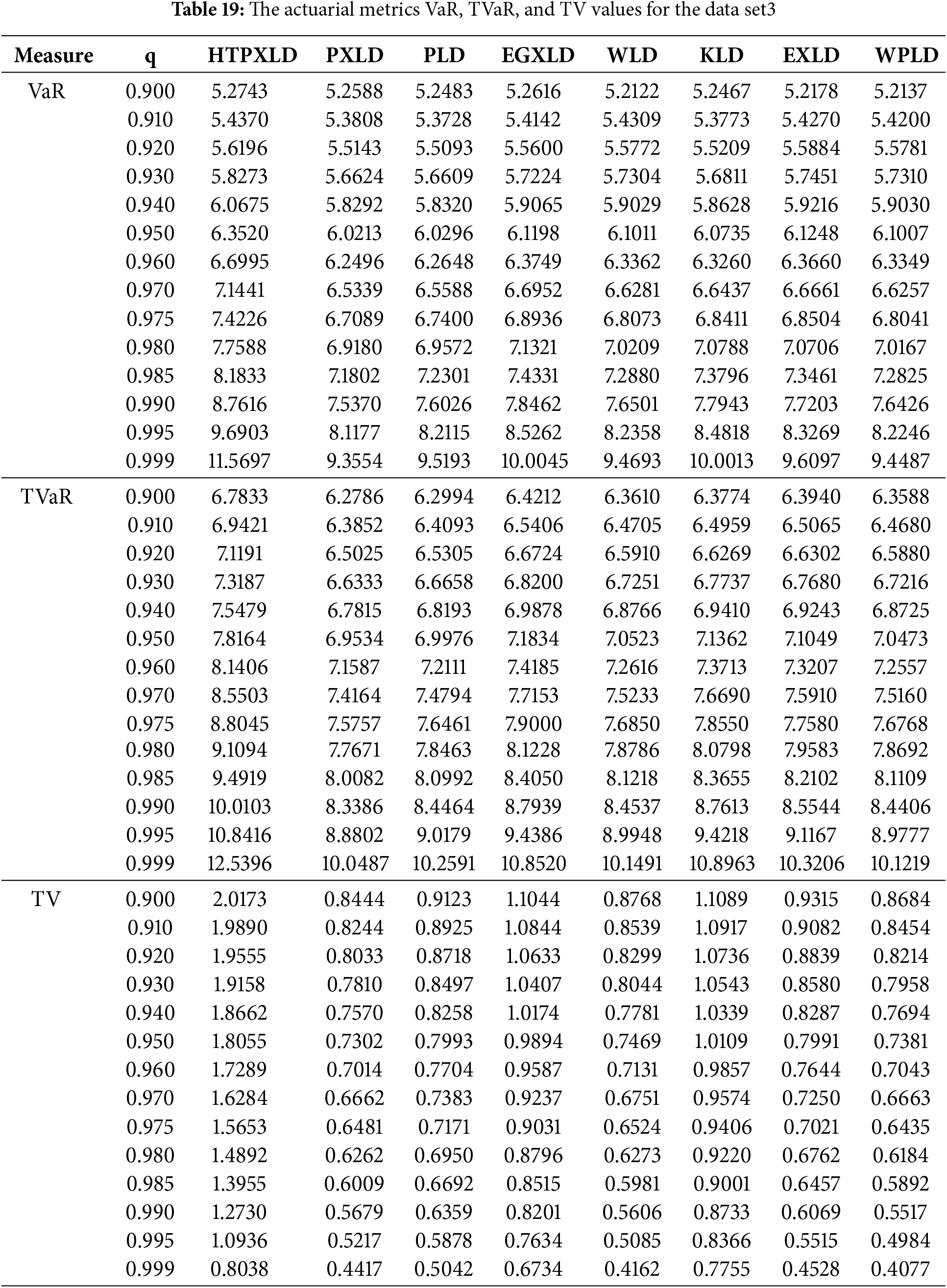
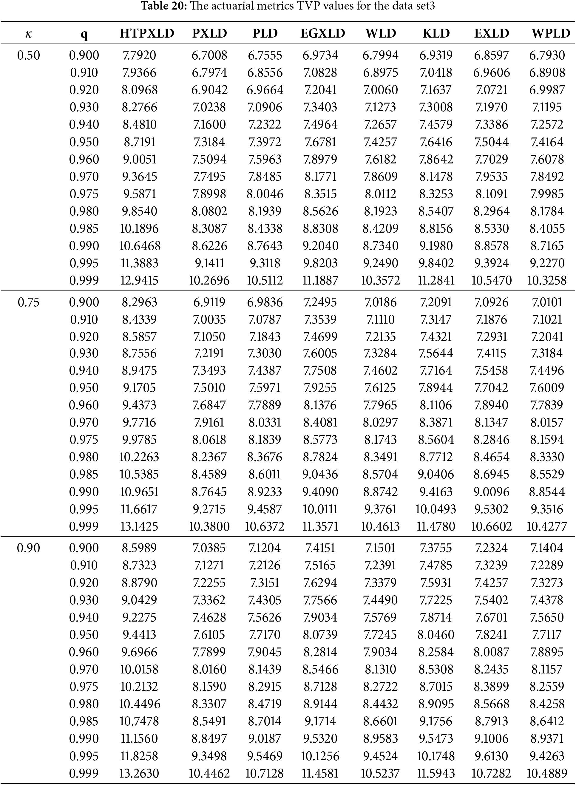
We find that for different significance levels and different values of , the HTPXLD model has greater values of the risk measures VaR, TVaR, TV, and TVP from Tables 19 and 20 and the Figs. 15 and 16. This suggests that compared to the PXLD, PLD, EGXLD, WLD, KLD, EXLD, and WPLD, the HTPXLD has a heavier tail.

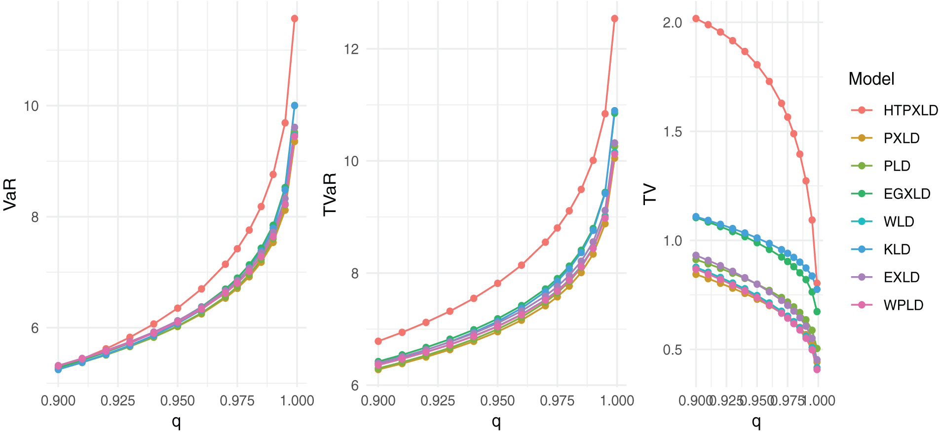
Figure 15: Competing model VaR, TVaR, and TV plots for the third dataset

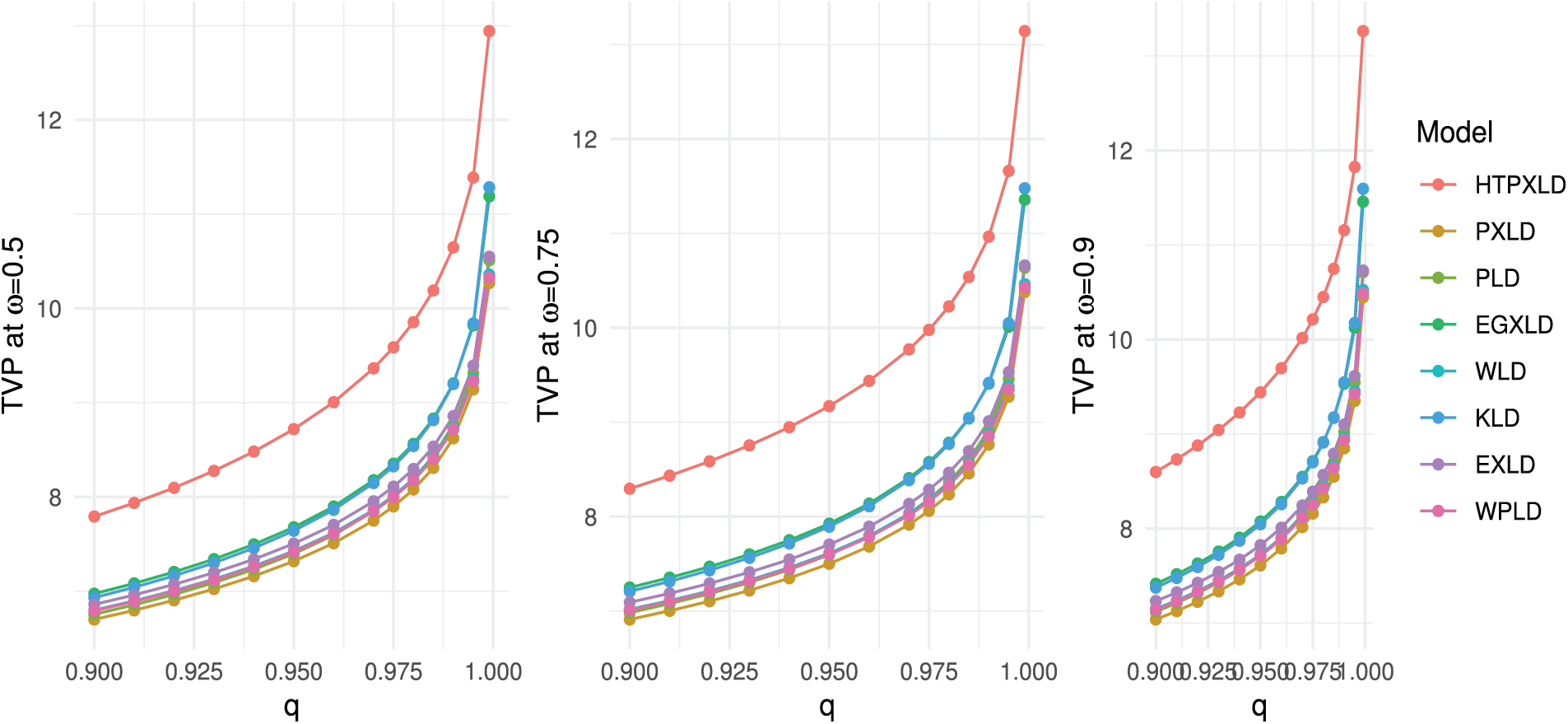
Figure 16: Competing model TVP plots for the third dataset

8  Conclusion

In the applied sciences, modeling heavy-tailed datasets is an important task, especially in domains like finance, medicine, and actuarial analysis. This paper constructs a novel heavy-tailed distribution by combining the PXLD with a heavy-tailed family. Especially when modeling leptokurtic lifespan data, that is, data with thicker tails this novel distribution presents a strongly modified version of the PXLD. With asymmetric forms and different degrees of peakedness, our suggested density gives more versatility, and its hazard rate function has various shapes. We delve into its statistical properties, deriving the quantile function, moments, incomplete moments, stochastic ordering, SS reliability parameter, and some extropy measures. We employ the ML procedure to estimate the model parameters. To assess the effectiveness of our proposed estimators, we conduct various simulation experiments. These experiments will evaluate the estimator’s performance using metrics like an average estimate, relative bias, bias, mean squared error, root mean squared error, average interval length, and coverage probability. We employ our suggested model to examine three real-world datasets to demonstrate its usefulness. The simulation analysis provided evidence that MLEs exhibit improved accuracy with increasing sample size. This is supported by the observed decrease in MSE, which is consistent with the theoretical expectation of parameter estimates converging toward their true values as the sample size grows. As sample numbers rise, the CP of the approximate CIs improves. As a result, we can be more certain that the actual parameter values fall inside the stated confidence intervals. Next, we evaluate its effectiveness in comparison to well-known rival models, emphasizing its benefits. A limitation of this study lies in its exclusive reliance on deriving point and interval estimates using the maximum likelihood method in the case of a complete sample. The simulation analysis presented in this work focuses specifically on scenarios with large sample sizes. Future studies should examine how well the HTPXLD performs in more realistic settings, such as those requiring ranked set sampling. Future studies should examine the HTPXLD’s performance on a larger variety of datasets with a range of attributes to fully evaluate its adaptability.

Acknowledgement: The authors thank King Saud University, Riyadh, Saudi Arabia for Supporting this research by Project Number (RSPD2025R548).

Funding Statement: This research is supported by researchers Supporting Project Number (RSPD2025R548), King Saud University, Riyadh, Saudi Arabia.

Author Contributions: Mohammed Elgarhy: Writing—original draft, Validation, Methodology, Formal analysis, Conceptualization, Writing—review, Investigation. Amal S. Hassan: Writing—original draft, Validation, Methodology, Formal analysis, Conceptualization, Writing—review, Investigation. Najwan Alsadat: Writing—original draft, Validation, Methodology, Formal analysis, Conceptualization, Writing—review, Investigation. Oluwafemi Samson Balogun: Writing—original draft, Validation, Methodology, Formal analysis, Conceptualization, Writing—review, Investigation. Ahmed W. Shawki: Writing—original draft, Validation, Methodology, Formal analysis, Conceptualization, Writing—review, Investigation. Ibrahim E. Ragab: Writing—original draft, Validation, Methodology, Formal analysis, Conceptualization, Writing—review, Investigation. All authors reviewed the results and approved the final version of the manuscript.

Availability of Data and Materials: All data generated or analyzed during this study are included in this published article.

Ethics Approval: Not applicable.

Conflicts of Interest: The authors declare no conflicts of interest to report regarding the present study.

References

1. Chouia S, Zeghdoudi H. The XLindley distribution: properties and application. J Stat Theory Appl. 2021;20(2):318–27. doi:10.2991/jsta.d.210607.001. [Google Scholar] [CrossRef]

2. Krishnarani S. On a power transformation of half-logistic distribution. J Probab Stat. 2016;2016(5):2084236. doi:10.1155/2016/2084236. [Google Scholar] [CrossRef]

3. Al-Omari A, Alhyasat K, Ibrahim K, Abu Bakar M. Power length-biased Suja distribution: properties and application. Electron J Appl Stat Anal. 2019;12(12):429–52. doi:10.1285/i20705948v12n2p429. [Google Scholar] [CrossRef]

4. Hassan AS, Nassar SG. Power lindley-G family. Ann Data Sci. 2019;6(2):189–210. doi:10.1007/s40745-018-0159-y. [Google Scholar] [CrossRef]

5. Shanker R, Shukla KK. Power weighted Sujayha distribution with properties and application to survival times of patients of head and neck cancer. Reliab Theory Appl. 2023;18(3):568–81. [Google Scholar]

6. Rady E, Hassanein W, Elhaddad T. The power Lomax distribution with an application to bladder cancer data. SpringerPlus. 2016;5:1–22. doi:10.1186/s40064-016-3464-y. [Google Scholar] [PubMed] [CrossRef]

7. Hassan AS, Nassr SG. Power lomax poisson distribution: properties and estimation. J Data Sci. 2018;16(1):105–28. doi:10.6339/JDS.201801_16(1).0007. [Google Scholar] [CrossRef]

8. Afify AZ, Gemeay AM, Alfaer NM, Cordeiro GM, Hafez EH. Power-modified kies-exponential distribution: properties, classical and bayesian inference with an application to engineering data. Entropy. 2022;24(7):883. doi:10.3390/e24070883. [Google Scholar] [PubMed] [CrossRef]

9. Hassan AS, Assar SM, Abd Elghaffar AM. Statistical properties and estimation of power-transmuted inverse Rayleigh distribution. Stat Trans New Series. 2020;21(3):1–20. doi:10.21307/stattrans-2020-046. [Google Scholar] [CrossRef]

10. Meriem B, Gemeay AM, Almetwally EM, Halim Z, Alshawarbeh E, Abdulrahman AT, et al. The power XLindley distribution: statistical inference, fuzzy reliability, and COVID-19 application. J Funct Spaces. 2022;2022(2):9094078. doi:10.1155/2022/9094078. [Google Scholar] [CrossRef]

11. Marshall AW, Olkin I. A new method for adding a parameter to a family of distributions with application to the exponential and Weibull families. Biometrika. 1997;84(3):641–52. doi:10.1093/biomet/84.3.641. [Google Scholar] [CrossRef]

12. Eugene N, Lee C, Famoye F. Beta-normal distribution and its applications. Commun Stat-Theor Meth. 2002;31(4):497–512. doi:10.1081/STA-120003130. [Google Scholar] [CrossRef]

13. Cordeiro GM, de Castro M. A new family of generalized distributions. J Stat Comput Simul. 2011;81(7):883–98. doi:10.1080/00949650903530745. [Google Scholar] [CrossRef]

14. Alzaatreh A, Lee C, Famoye F. A new method for generating families of continuous distributions. METRON. 2013;71(1):63–79. doi:10.1007/s40300-013-0007-y. [Google Scholar] [CrossRef]

15. Bourguignon M, Silva RB, Cordeiro GM. The Weibull-G family of probability distributions. J Data Sci. 2014;12(1):53–68. doi:10.6339/JDS.201401_12(1).0004. [Google Scholar] [CrossRef]

16. Kumar D, Singh U, Singh SK. A method of proposing new distribution and its application to bladder cancer patient data. J Stat Probab Lett. 2015;2:235–45. [Google Scholar]

17. Cordeiro GM, Alizadeh M, Diniz Marinho PR. The type I half-logistic family of distributions. J Stat Comput Simul. 2015;86(4):707–28. doi:10.1080/00949655.2015.1031233. [Google Scholar] [CrossRef]

18. Cordeiro GM, Alizadeh M, Ortega EMM. The exponentiated half-logistic family of distributions: properties and applications. J Probab Stat. 2014;2014(1):864396. doi:10.1155/2014/864396. [Google Scholar] [CrossRef]

19. Bodhisuwan W, Sangsanit Y. The Topp-Leone generator of distributions: properties and inferences. Songklanakarin J Sci Technol. 2016;38(5):537–48. [Google Scholar]

20. Alizadeh M, Cordeiro GM, Pinho LGB, Ghosh I. The Gompertz-G family of distributions. J Stat Theory Pract. 2016;11(1):179–207. doi:10.1080/15598608.2016.1267668. [Google Scholar] [CrossRef]

21. Chipepa F, Oluyede B, Makubate B, Fagbamigbe AF. The beta odd Lindley-G family of distributions with applications. J Probab Stat Sci. 2019;17(1):51–83. [Google Scholar]

22. Hassan AS, Sabry MAH, Elsehery AM. A new probability distribution family arising from truncated power lomax distribution with application to weibull model. Pak J Stat Oper Res. 2020;16(4):661–74. doi:10.18187/pjsor.v16i4.3442. [Google Scholar] [CrossRef]

23. Kavya P, Manoharan M. Some parsimonious models for lifetimes and applications. J Stat Comput Simul. 2021;91:3693–708. doi:10.1080/00949655.2021.1946064. [Google Scholar] [CrossRef]

24. Hassan AS, Al-Omari AI, Hassan RR, Alomani G. The odd inverted Topp Leone H family of distributions: estimation and applications. J Radiat Res Appl Sci. 2022;15(3):365–79. doi:10.1016/j.jrras.2022.08.006. [Google Scholar] [CrossRef]

25. Korkmaz MÇ., Cordeiro GM, Yousof HM, Pescim RR, Afify AZ, Nadarajah S. The Weibull Marshall-Olkin family: regression model and application to censored data. Commun Stat-Theor Meth. 2018;48(16):4171–94. doi:10.1080/03610926.2018.1490430. [Google Scholar] [CrossRef]

26. Souza L, de Oliveira WR, de Brito CCR, Chesneau C, Fernandes R, Ferreira TAE. Sec-G class of distributions: properties and applications. Symmetry. 2022;14(2):299. doi:10.3390/sym14020299. [Google Scholar] [CrossRef]

27. Hassan AS, Alsadat N, Chesneau C, Shawki AW. A novel weighted family of probability distributions with applications to world natural gas, oil, and gold reserves. Mathem Biosci Eng. 2023;20(11):19871–911. doi:10.3934/mbe.2023880. [Google Scholar] [PubMed] [CrossRef]

28. Shah Z, Khan DM, Khan Z, Faiz N, Hussain S, Anwar A, et al. A new generalized logarithmic-X family of distributions with biomedical data analysis. Appl Sci. 2023;13(6):3668. doi:10.3390/app13063668. [Google Scholar] [CrossRef]

29. Musekwa RR, Gabaitiri L, Makubate B. A new technique to generate families of continuous distributions. Revista Colombiana De Estadistica. 2024;47(2):329–54. doi:10.15446/rce.v47n2.112245. [Google Scholar] [CrossRef]

30. Makubate B, Chipepa F, Oluyede B, Moagi G. The Marshall-Olkin-exponentiated half logistic-G family of distributions: model, properties and applications. J Statist Manag Syst. 2024;27(7):1243–59. doi:10.47974/JSMS-854. [Google Scholar] [CrossRef]

31. Ahmad Z, Mahmoudi E, Hamedani CG, Kharazmi O. New methods to define heavy-tailed distributions with applications to insurance data. J Taibah Univ Sci. 2020;14(1):359–82. doi:10.1080/16583655.2020.1741942. [Google Scholar] [CrossRef]

32. Ahmad Z, Mahmoudi E, Hamedani GG. A class of claim distributions: properties, characterizations and applications to insurance claim data. Commun Stat-Theor Meth. 2020;51(7):2183–208. doi:10.1080/03610926.2020.1772306. [Google Scholar] [CrossRef]

33. Nadarajah S, Lyu J. New discrete heavy tailed distributions as models for insurance data. PLoS One. 2025;18(5):e0285183. doi:10.1371/journal.pone.0285183. [Google Scholar] [PubMed] [CrossRef]

34. Nair J, Wierman A, Zwart B. The fundamentals of heavy tails: properties, emergence, and estimation. Cambridge, UK: Cambridge University Press; 2022. doi:10.1017/9781009053730. [Google Scholar] [CrossRef]

35. McNeil AJ. Estimating the tails of loss severity distributions using extreme value theory. ASTIN Bull. 1997;27(1):117–37. doi:10.2143/AST.27.1.563210. [Google Scholar] [CrossRef]

36. Olmos NM, Gomez-Deniz E, Venegas O. The heavy-tailed gleser model: properties, estimation, and applications. Mathematics. 2022;10(23):4577. doi:10.3390/math10234577. [Google Scholar] [CrossRef]

37. Zhao W, Khosa SK, Ahmad Z, Aslam M, Affy AZ. Type-I heavy tailed family with applications in medicine, engineering and insurance. PLoS One. 2020;15(8):e0237462. doi:10.1371/journal.pone.0237462. [Google Scholar] [PubMed] [CrossRef]

38. Moakofi T, Oluyede B. The type I heavy-tailed odd power generalized Weibull-G family of distributions with applications. Commun Fac Sci Univ Ankara Series A1 Math Stat. 2023;72(4):921–58. doi:10.31801/cfsuasmas.1195058. [Google Scholar] [CrossRef]

39. Moakofi T, Oluyede B, Tlhaloganyang B, Puoetsile A. A new family of heavy-tailed generalized Topp-Leone-G distributions with applications. Pak J Stat Oper Res. 2024;20(2):233–60. doi:10.18187/pjsor.v20i2.4458. [Google Scholar] [CrossRef]

40. Ahmad Z, Mahmoudi E, Dey S. A new family of heavy tailed distributions with an application to the heavy tailed insurance loss data. Commun Statist-Simulat Computat. 2020;51(8):4372–95. doi:10.1080/03610918.2020.1741623. [Google Scholar] [CrossRef]

41. Corless RM, Gonnet GH, Hare DE, Jeffrey DJ, Knuth DE. On the Lambert W function. Adv Comput Math. 1995;5(1):329–59. doi:10.1007/BF02124750. [Google Scholar] [CrossRef]

42. Kenney JF, Keeping E. Mathematics of statistics (part one). Louisville, KY, USA: D. Van Nostrand Company, Inc.; 1962. [Google Scholar]

43. Moors JJA. A quantile alternative for kurtosis. J Royal Stat Soc: Series D (Stat). 1988;37(1):25–32. [Google Scholar]

44. Butler RJ, McDonald JB. Using incomplete moments to measure inequality. J Econom. 1989;42(1):109–19. doi:10.1016/0304-4076(89)90079-1. [Google Scholar] [CrossRef]

45. Shaked M, Shanthikumar JG. Stochastic orders and their applications. New York, NY, USA: Academic Press; 1994. [Google Scholar]

46. Shannon CE. A mathematical theory of communication. Bell Syst Tech J. 1948;27(3):379–423. doi:10.1002/j.1538-7305.1948.tb01338.x. [Google Scholar] [CrossRef]

47. Lad F, Sanfilippo G, Agr G. Extropy: complementary dual of entropy. Statist Sci. 2015;30(1):40–58. doi:10.1214/14-STS430. [Google Scholar] [CrossRef]

48. Balakrishnan N, Buono F, Longobardi M. On weighted extropies. Commun Stat-Theor Meth. 2022;51(18):6250–67. doi:10.1080/03610926.2020.1860222. [Google Scholar] [CrossRef]

49. Artzner P. Application of coherent risk measures to capital requirements in insurance. N Am Actuar J. 1999;3(2):11–25. doi:10.1080/10920277.1999.10595795. [Google Scholar] [CrossRef]

50. Landsman Z. On the tail mean-variance optimal portfolio selection. Insur Math Econ. 2010;46(3):547–53. doi:10.1016/j.insmatheco.2010.02.001. [Google Scholar] [CrossRef]

51. Lindley DV. Fiducial distributions and Bayes’ theorem. J Royal Stat Soc: Series B (Meth). 1958;20(1):102–10. doi:10.1111/j.2517-6161.1958.tb00278.x. [Google Scholar] [CrossRef]

52. Musekwa RR, Makubate B. A flexible generalized XLindley distribution with application to engineering. Sci Afr. 2024;24(2):e02192. doi:10.1016/j.sciaf.2024.e02192. [Google Scholar] [CrossRef]

53. Rajitha CS, Akhilnath A. Generalization of the Lindley distribution with application to COVID-19 data. Int J Data Sci Anal. 2022;23:1–21. doi:10.1007/s41060-022-00369-2. [Google Scholar] [PubMed] [CrossRef]

54. Abdelmoezz S, Mohamed SM. The kumaraswamy lindley regression model with application on the Egyptian stock exchange: numerical study, regression model. Jurnal Matematika, Statistika Dan Komputasi. 2021;18(1):1–11. doi:10.20956/j.v18i1.14784. [Google Scholar] [CrossRef]

55. MirMostafaee SMTK, Alizadeh M, Altun E, Nadarajah S. The exponentiated generalized power Lindley distribution: properties and applications. Appl Mathem-J Chin Univ. 2019;34(2):127–48. doi:10.1007/s11766-019-3515-6. [Google Scholar] [CrossRef]

56. Ghitany ME, Al-Mutairi DK, Balakrishnan N, Al-Enezi LJ. Power Lindley distribution and associated inference. Computat Statist Data Analy. 2013;64(9):20–33. doi:10.1016/j.csda.2013.02.026. [Google Scholar] [CrossRef]

57. Asgharzadeh AKBAR, Nadarajah S, Sharafi F. Weibull Lindley distribution. Revstat-Statist J. 2018;16(1):87–113. doi:10.57805/revstat.v16i1.234. [Google Scholar] [CrossRef]

58. Bakouch HS, Al-Zahrani BM, Al-Shomrani AA, Marchi VA, Louzada F. An extended Lindley distribution. J Korean Statist Soc. 2012;41(1):75–85. doi:10.1016/j.jkss.2011.06.002. [Google Scholar] [CrossRef]

59. Lemonte AJ, Barreto-Souza W, Cordeiro GM. The exponentiated Kumaraswamy distribution and its log-transform. Braz J Probab Stat. 2013;27(1):31–53. doi:10.1214/11-BJPS149. [Google Scholar] [CrossRef]

60. Lee ET, Wang J. Statistical methods for survival data analysis. New York, NY, USA: John Wiley & Sons; 2003. Vol. 476. [Google Scholar]