A Robust GNSS Navigation Filter Based on Maximum Correntropy Criterion with Variational Bayesian for Adaptivity

Dah-Jing Jwo; Yi Chang; Ta-Shun Cho

doi:10.32604/cmes.2025.057825

icon Open Access

ARTICLE

A Robust GNSS Navigation Filter Based on Maximum Correntropy Criterion with Variational Bayesian for Adaptivity

Dah-Jing Jwo^1,2,*, Yi Chang², Ta-Shun Cho³

1 Department of Communications, Navigation and Control Engineering, National Taiwan Ocean University, Keelung, 202301, Taiwan
2 Department of Electrical Engineering, National Taiwan Ocean University, Keelung, 202301, Taiwan
3 Department of Business Administration, Asia University, 500 Liufeng Road, Wufeng, Taichung, 41354, Taiwan

* Corresponding Author: Dah-Jing Jwo. Email: email

(This article belongs to the Special Issue: Scientific Computing and Its Application to Engineering Problems)

Computer Modeling in Engineering & Sciences 2025, 142(3), 2771-2789. https://doi.org/10.32604/cmes.2025.057825

Received 28 August 2024; Accepted 14 January 2025; Issue published 03 March 2025

Abstract

In this paper, an advanced satellite navigation filter design, referred to as the Variational Bayesian Maximum Correntropy Extended Kalman Filter (VBMCEKF), is introduced to enhance robustness and adaptability in scenarios with non-Gaussian noise and heavy-tailed outliers. The proposed design modifies the extended Kalman filter (EKF) for the global navigation satellite system (GNSS), integrating the maximum correntropy criterion (MCC) and the variational Bayesian (VB) method. This adaptive algorithm effectively reduces non-line-of-sight (NLOS) reception contamination and improves estimation accuracy, particularly in time-varying GNSS measurements. Experimental results show that the proposed method significantly outperforms conventional approaches in estimation accuracy under heavy-tailed outliers and non-Gaussian noise. By combining MCC with VB approximation for real-time noise covariance estimation using fixed-point iteration, the VBMCEKF achieves superior filtering performance in challenging GNSS conditions. The method’s adaptability and precision make it ideal for improving satellite navigation performance in stochastic environments.

Keywords

Maximum correntropy criterion; variational Bayesian; extended Kalman filter; GNSS

1 Introduction

Multipath interference and non-line-of-sight (NLOS) reception are the major sources of error for GNSS (global navigation satellite system) positioning systems, such as the Global Positioning System (GPS) in an urban environment [1]. These elements lead to measurement outliers with heavy tails, which impact the performance. The traditional mean squared error (MSE) criteria work well when the Gaussian noise is involved, but it performs poorly when there is non-Gaussian noise. Therefore, the Gaussian noise in the navigation state estimation techniques based on the extended Kalman filter (EKF) has been considered. In non-Gaussian noise environments, the practical GNSS navigation applications have made algorithm resilience a critical concern. Correntropy has been used to replace the MSE information [2] to capture more statistical information in Information Theoretic Learning (ITL). Consequently, the correntropy-based algorithms are more resilient to non-Gaussian noise [3]. The maximum correntropy criteria (MCC)-based technique maximizes the correntropy between the system’s output and the intended signal in order to recursively update equations. Because the statistics of measurement noise alters, the state estimation performance for GNSS navigation processing utilizing the Kalman filters family is also affected [4,5].

In recent years, numerous studies have explored the use of MCC and variational Bayesian (VB)-based techniques for addressing non-Gaussian noise in GNSS environments. Despite the improvements in robustness, these approaches often struggle in environments with rapidly changing noise characteristics and heavy-tailed outliers, particularly in urban settings prone to multipath interference [6]. Existing methods are either limited by fixed noise models or lack the adaptability required for real-time applications, leading to degraded positioning accuracy under dynamic conditions. To address these challenges, our proposed method introduces a novel combination of MCC with real-time noise covariance estimation via VB approximation. This technique is specifically tailored for urban GNSS environments, where traditional filters and even some MCC-based approaches face difficulties [7,8]. Our approach enhances both robustness and adaptability by iteratively updating the noise covariance during navigation, ensuring superior performance in scenarios with time-varying non-Gaussian noise. The major contribution of this work is the application of fixed-point iteration within the MCC framework, allowing for more precise and dynamic noise covariance estimation. This, in turn, directly improves the accuracy of state estimation, particularly in challenging multipath environments where existing methods underperform. By overcoming the limitations of previous MCC-based algorithms, our method offers a more effective filtering solution for real-world GNSS applications, demonstrating resilience in handling dynamic noise and heavy-tailed outliers, which are prevalent in urban GNSS environments [9].

In addition to experimental validation, it is essential to understand the theoretical foundations that underpin the superior performance of combined MCC and VB approaches over traditional EKF methods. The fundamental limitation of EKF lies in its inherent assumption of Gaussian noise distributions and its reliance on second-order statistics. This assumption becomes problematic in GNSS environments where non-Gaussian noise and outliers are common due to multipath effects and NLOS reception. While EKF minimizes the mean squared error, which can be disproportionately affected by outliers due to its quadratic nature, MCC employs a more robust cost function through its kernel-based approach. The Gaussian kernel in MCC naturally bounds the influence of outliers, providing theoretical justification for better performance in heavy-tailed noise environments. Moreover, the integration of VB methodology provides a theoretical framework for adaptive noise estimation that addresses another key limitation of traditional EKF—its dependence on fixed, pre-specified noise statistics. By minimizing the Kullback-Leibler divergence between the true posterior and its variational approximation, VB enables online adaptation of noise parameters, theoretically guaranteeing improved performance under time-varying conditions. This theoretical advantage becomes particularly significant in urban GNSS environments where noise characteristics can change rapidly due to varying satellite geometry and signal propagation conditions.

It is common to identify the heavy-tailed outliers and non-Gaussian noise in measurements taken with the GPS. During transmission, data loss may be caused by multipath effects and occasional noise. These elements lead to measurement outliers, which degrades the system performance. The studies are carried out based on the navigation state estimation strategies for Gaussian noise using an enhanced Kalman filter. For practical applications, it performs significantly worse with the non-Gaussian noise. The robust MCC was proposed by Liu et al. [10], where the application of the adaptive filtering method is significantly affected by the processing of non-Gaussian signals. The optimization of non-Gaussian satellite navigation systems using the maximum correntropy extended Kalman filter (MCEKF) played a vital role in many applications [11]. In practical applications, variational Bayesian (VB) is a quick and precise approximation technique that handles quite complex probability distributions [12]. Many researchers have studied the MCEKF for GPS navigation in a non-Gaussian environment, which reveals the study of adaptive kernel size with better performance accuracy [13]. Furthermore, the GPS navigation state is computed using non-Gaussian noise or a heavy tail anomalous noise value within the framework of the MCC, which aids in resolving the filtering design constraint. Recently, filtering issues have been tackled with machine learning techniques based on VB learning to improve GPS navigation accuracy [14,15]. For the most complex models, it is difficult to calculate the precise posterior distribution. To obtain an accurate distribution, therefore variational distribution has been added to the system model. This feature’s goal is to minimize the difference between the posterior probability density function (pdf) and its variational distribution, or the Kullback-Leibler divergence (KLD), or relative entropy [16,17].

In this present work, the non-Gaussian measurement interference has been reduced through the application of the maximum correntropy criterion. Using the fixed-point iteration, the VB approximation is used to estimate the noise covariance in real time. With the predicted covariance for the measurement noise, which can be modified with an EKF, the combined MCC and VB technique is suggested in this investigation [18,19]. Furthermore, in a multipath noise environment, this strong adaptive algorithm technique offers better estimation accuracy. Furthermore, with excellent estimation accuracy, the aforementioned features can be generalized to improve the performance of satellite navigation in stochastic systems. Specifically, the VBMCEKF framework leverages the advantages of both VB approximation and MCC-based noise handling. By dynamically adjusting the kernel bandwidth, the method can adapt to rapidly changing measurement conditions and stochastic noise variations. This adaptability is crucial for satellite navigation systems that must operate in unpredictable environments with non-Gaussian noise, such as urban canyons or dense foliage, where multipath effects and outliers can severely degrade performance. This is an example of adaptivity being achieved by the use of VB learning based on the probabilistic technique to estimate the time-varying noise covariance matrices. In each updated step, the system state and time-varying measurement noise are identified as random variables and are estimated. The VB approach uses VB learning to treat the time-varying measurement noises and iterates the estimate process each time to approximate the real joint posterior distribution of the state. A recursive method for approximating the true posterior of the noise and the states is provided by VB learning using the probabilistic approach.

2 The Extended Kalman Filter Based on Maximum Correntropy Criterion

The study of information theory gave rise to the novel similarity monitoring technique known as correntropy [20]. These are starting to recognize correntropy as a stable nonlinear identity metric in kernel space in the fields of machine learning and signal processing. It is effectively used in random signal processing, primarily with the MCC.

$Vσ(X,Y)=E[κσ(X,Y)]=∫κσ(x,y)fXY(x,y)dxdy$ (1)

The correntropy function is expressed as $Vσ(X,Y)=E[κσ(X−Y)]$ , where $E[⋅]$ represents the expected value, $κσ(⋅)$ is the Mercer kernel function with translation invariance, and $σ>0$ is the kernel bandwidth. The commonly used Mercer kernel function is the Gaussian kernel function, which is defined as follows:

$κσ(x−y)=Gσ(x−y)=12πσexp⁡(−((x−y)22σ2))$ (2)

Correntropy has been effectively utilized as a nonlinear similarity measure in signal processing and machine learning by maximizing the correntropy $V^$ between the model output and the intended reaction.

$V^σ(X,Y)=1N∑i=1NGσ(ei)=1N∑i=1Nκσ(xi−yi)$ (3)

In addition, higher-order terms can be disregarded since system performance will deteriorate as the kernel bandwidth gets closer to infinity. The least mean squared error and greatest correntropy criteria will then be similar because they will roughly equal each other at this time. The classical Kalman filter theory, which uses the MSE as a state estimation method for linear Gaussian systems, is the basic foundation for the MCEKF. It is appropriate for errors with a Gaussian distribution since it not only analyses the second moment of the error distribution but was also created under the assumption of a Gaussian distribution. The EKF approach is combined with the MCC, which significantly improves performance when working with non-Gaussian signals. When processing nonlinear and non-Gaussian noise sources, this characteristic shows benefits. Because of its dependability, the maximum correntropy is frequently utilized in machine learning and signal processing. The nonlinear system state model and observation model are as follows:

$xk=f(xk−1)+wk−1$ (4)

$zk=h(xk)+vk$ (5)

where the state vector $xk∈Rn$ , $f(⋅)$ is a nonlinear system function, the measurement vector $zk∈Rm$ , $h(⋅)$ is the nonlinear system observation function. Both the vectors $wk−1$ and $vk$ are zero mean Gaussian white sequences having zero cross-correlation with each other.

To modify the degree of similarity between two random variables, the kernel bandwidth is an important variable. We can adjust the kernel bandwidth to change the greatest correntropy in the local range, which measures the degree of similarity. The maximum correntropy localized similarity increases to global similarity and collapses into the conventional mean squared error criterion as the kernel bandwidth approaches positive infinity. The maximum correntropy extended Kalman filter is derived by minimizing the following objective function:

$Jk=Gσ(||x^k−x^k|k−1||Pk|k−1−1)+Gσ(||zi,k−h(x^k)||Rk−1)$ (6)

where $xk∈Rn$ and $zk∈Rm$ are the estimated state vector and measurement vector, respectively. The Gaussian kernel function is given by $Gσ(||⋅||)=exp⁡(−||⋅||A22σ2)$ , where $||⋅||A$ represents the weighted 2-norm of the vector, and thus $||x||A2=xTAx$ , and $σ$ is the kernel bandwidth. The size of the traditional kernel bandwidth is selected manually.

The nonlinear measurement function must be linearized by Taylor series expansion in order to minimize Eq. (6) with respect to $xk$ . Compute the derivative with respect to $xk$ in order to minimize this cost function via

$∂Jk∂xk=0$ (7)

which leads to

$1σ2Gσ(||zk−h(x^k)||Rk−1)HkTRk−1(zk−h(x^k))−1σ2Gσ(||x^k−x^k|k−1||Pk|k−1−1)Pk|k−1−1(x^k−x^k|k−1)=0$ (8)

Eq. (7) represents the condition for minimizing the cost function with respect to $xk$ , and taking the derivative as shown leads to Eq. (8).

The solution can be obtained by solving

$Gσ(||x^k−x^k|k−1||Pk|k−1−1)Pk|k−1−1(x^k−x^k|k−1)=Gσ(||zk−h(x^k)||Rk−1)HkTRk−1(zk−h(x^k))$ (9)

Eq. (8) is then rearranged and solved to express the solution in terms of $Pk|k−1−1$ , leading to Eq. (9). This equation now shows the relationship between the prior and the measurement update step.

$Pk|k−1−1x^k=Pk|k−1−1x^k|k−1+Gσ(||zk−h(x^k)||Rk−1)Gσ(||x^k−x^k|k−1||Pk|k−1−1)HkTRk−1(zk−h(x^k))$ (10)

Eq. (10) follows by isolating $Pk|k−1−1$ on one side of the equation. This equation indicates how the measurement affects the prior covariance to produce the updated estimate.

Let $Ck=Gσ(||zk−h(x^k)||Rk−1)Gσ(||x^k−x^k|k−1||Pk|k−1−1)$ , and $Gσ(||x^k−x^k|k−1||Pk|k−1−1)=Gσ(||0||Pk|k−1−1)=1$ . Introducing the substitution made for $Ck$ in Eq. (10) leads to a simplification in the resulting equation. This substitution reduces the complexity of the expression, simplifying the final computation of the updated state estimate. $Gσ$ is the kernel function used to measure the similarity or distance between two estimates. When the two estimates are very close, $Gσ$ approaches 1, indicating that they are identical in this metric.

With the following definition:

$Pk|k−1−1x^k=Pk|k−1−1x^k|k−1+CkHkTRk−1(zk−h(x^k))$ (11)

Before Eq. (12), state that the correction filter derived approximates $x^k$ using the prior estimate $x^k|k−1$ , and this is done to ensure consistency in the estimation process.

The correntropy filter is derived by approximating $x^k≈x^k|k−1$ on the right-hand side of Eq. (11).

$CkHkTRk−1Hkx^k−CkHkTRk−1Hkx^k|k−1=0$ (12)

Eq. (12) essentially sets up the condition for the filter to correct the estimate based on the measurements.

$Pk|k−1−1x^k+CkHkTRk−1Hkx^k=Pk|k−1−1x^k|k−1+CkHkTRk−1(zk−h(x^k))+CkHkTRk−1Hkx^k|k−1$ (13)

Eq. (13) can be derived as

$x^k=x^k|k−1+(Pk|k−1−1+CkHkTRk−1Hk)−1CkHkTRk−1(zk−h(x^k))$ (14)

The estimator for the updated state is directly obtained from Eq. (14). The update equation refines the previous estimate by incorporating the measurement residual, adjusting the state estimate as follows:

$x^k=x^k|k−1+Kk(zk−h(x^k))$ (15)

where the Kalman gain $Kk$ is given by

$Kk=(Pk|k−1−1+CkHkTRk−1Hk)−1CkHkTRk−1$ (16)

Moreover, the posterior covariance matrix can be updated by

$Pk=(I−KkHk)Pk|k−1(I−KkHk)T+KkRkKkT$ (17)

The MCEKF doesn’t have numerical problems in the face of large outliers. When $Ck$ gets close to zero, the filter gain becomes very small. As a result, the MCEKF is resistant to measurement outliers. However, it is not effective when the measurement noise covariance is unknown or time-varying.

3 Variational Bayesian Extended Kalman Filter Based on Maximum Correntropy Criterion

In this section, the variational Bayesian extended Kalman filter based on the maximum correntropy criterion (VBMCEKF) is introduced for GNSS navigation processing. This technique is based on the modified extended Kalman filter involving VB adaptation and MCC optimization. The modified joint approach to satellite navigation design is given in the context of non-Gaussian and heavy-tail outlier noise scenarios.

There are similarities in state estimation for the classical Kalman filters family in terms of prediction, update procedures, and measurement noise variance estimates, respectively [21,22]. Only a correlation exists between the current estimate and the earlier estimate. The algorithm also performed $N$ iterations of measurement updates to enhance the correction of the state estimate and variance against noise. Through iterative computation, the variational Bayesian parameters estimate forms an integral part of the gradient descent technique, where convergence is evaluated by comparing the lower bounds of two subsequent rounds. When the difference is less than a preset threshold, it is possible to predict when the algorithm will converge and obtain the estimation result. Reducing a complex Bayesian estimate’s probability density into a few more manageable probability densities is the fundamental idea of variational Bayesian estimation. Assuming $Rk$ the problem involves calculating a conditional probability density $p(xk,Rk|z1:k)$ based on $z1:k$ . The EKF can provide a result if $Rk$ is known. However, when $Rk$ is unknown or varies over time, it can be challenging to obtain a statistical result.

In order to achieve self-adaptation, VBMCEKF was employed to predict the measurement noise covariance using the VB technique and MCC was utilized to improve robustness and reduce the impact of outliers. Since $Ck$ is related to the measurement of noise covariance, the VB method is beneficial for repressing outliers by estimating noise covariance. In the MCC framework, $Ck$ plays a key role in scaling the influence of outliers and dynamically adjusting the measurement noise covariance based on the similarity between the predicted and measured states. By retaining $Ck$ , VBMCEKF leverages MCC’s strength in handling non-Gaussian noise, enabling effective outlier suppression and adaptive noise covariance estimation. This allows the filter to maintain robustness while improving estimation accuracy in varying noise environments.

Since $Ck$ is related to the measurement of noise covariance, the VB method is beneficial for repressing outliers by estimating noise covariance. In the MCC framework, $Ck$ plays a key role in scaling the influence of outliers and dynamically adjusting the measurement noise covariance based on the similarity between the predicted and measured states. By retaining $Ck$ , VBMCEKF leverages MCC’s strength in handling non-Gaussian noise, enabling effective outlier suppression and adaptive noise covariance estimation. This allows the filter to maintain robustness while improving estimation accuracy in varying noise environments [23,24].

Additionally, the MCC is effective in mitigating interference caused by non-Gaussian measurement noise. A fixed-point iterative method is used to integrate MCC and VB in order to modify the measurement noise covariance that is acquired [25,26]. The VB approximation is used to identify the measurement noise to estimate the measurement noise covariance, and the MCC method is beneficial in reducing interference caused by non-Gaussian measurement noise. Therefore, the measurement noise covariance will be estimated using the VB technique to provide self-adaptability, and the MCC will be used to suppress outliers to provide robustness. Through iterative calculation, the VB parameters estimate is essentially a component of the gradient descent technique, where convergence is evaluated by comparing the lower bounds of two subsequent rounds. However, selecting the kernel bandwidth has never been easy and is frequently based on inaccurate experimental and real data.

To increase MCEKF’s accuracy and stability, the appropriate kernel bandwidth is a crucial element. The filter receives more outliers when the kernel bandwidth is wider; conversely, a narrower kernel bandwidth results in a slower convergence or, in certain situations, a divergence of the filter. The adaptive kernel bandwidth in the MCC algorithm helps overcome the trade-off between convergence speed and the accuracy of steady-state results in the fixed kernel bandwidth MCC algorithm. The VBMCEKF method suggests the following approach for adjusting the adaptive kernel bandwidth:

$σμ,k=(||υμ,k(υμ,k)T||R^μ,k−1−1+Hμ,kPk|k−1HμT)$ (18)

where $υμ,k=zμ,k−h(x^μ,k|k−1)$ and the parameter $μ∈{1,…,m}$ represents the dimension index of the matrix. In this formula, $|υμ,k(υμ,k)T||R^μ,k−1−1$ represents the innovation, which indicates the difference between the predicted and measured states. A large innovation signals outliers or abrupt changes, requiring a wider kernel bandwidth. Conversely, a smaller innovation allows for a reduced bandwidth, facilitating faster convergence. The term $Hμ,kPk|k−1HμT$ reflects state covariance, with greater uncertainty demanding a wider bandwidth. By incorporating both innovation and covariance, the adaptive mechanism adjusts the kernel bandwidth to balance outlier suppression and estimation accuracy.

By employing adaptive kernel bandwidth, both the weighted innovation term and the weighted covariance of the estimation error are taken into account. This approach offers the advantage of tailored adaptation to each observation dimension, allowing the filter to respond effectively to varying noise levels and outlier distributions. However, while the introduction of an adaptive kernel bandwidth mechanism to fine-tune the correntropy gain is a promising aspect, further details are needed on how this mechanism adapts to different situations or what criteria are used to adjust the correntropy gain. Providing a more in-depth explanation of these adaptive mechanisms would enhance the understanding of their robustness and efficacy across various scenarios. If the prior distribution of the parameter to be estimated is selected from the conjugate exponential family, the resulting approximated distribution will retain the same form as the prior distribution, with adjustments to the parameters. In variational Bayesian theory, the inverse Wishart (IW) distribution is typically chosen as the conjugate prior for Gaussian covariance matrices. The prior distributions of $Pk|k−1$ and $Rk$ , the Gaussian covariance matrices, follow inverse Wishart distributions. Specifically, the distributions $p(Pk|k−1|z1:k−1)$ and $p(Rk|z1:k−1)$ are expressed as

$p(Pk|k−1|z1:k−1)=IW(Pk|k−1;t^k|k−1,T^k|k−1)$ (19)

and

$p(Rk|z1:k−1)=IW(Rk;u^k|k−1,U^k|k−1)$ (20)

In order to obtain the priori information of $Pk|k−1$ , its mean value is set to the nominal prediction error covariance matrix $P~k|k−1$ , that is

$P~k|k−1=λΦk−1Pk−1Φk−1T+Q~k−1$ (21)

where $Q~k−1$ represents the process noise covariance matrix, and $λ$ is an artificial threshold introduced to ensure numerical stability. Let $t^k|k−1=n+τ+1$ , where $τ$ denotes a tuning parameter. The degrees of freedom for the inverse Wishart distribution are updated iteratively, as shown by the following equation:

$P~k|k−1=T^k|k−1t^k|k−1−n−1$ (22)

This equation provides a way to iteratively adjust the degrees of freedom, which influences the shape of the inverse Wishart distribution as new data is incorporated. The inverse scaling matrix is also updated as part of the recursive process.

$T^k|k−1=τP~k|k−1$ (23)

This update adjusts the inverse scaling matrix based on the nominal prediction error covariance matrix, ensuring that it incorporates the most recent information from the prediction step. When employing the heuristic approach, the prior parameters $u^k|k−1$ and $U^k|k−1$ are updated using the following equations:

$u^k|k−1=ρ(u^k−1|k−1−m−1)+m+1$ (24)

and

$U^k|k−1=ρU^k−1|k−1$ (25)

where $ρ∈(0,1]$ denotes the forgetting factor, which controls the balance between the contribution of prior information and new measurements. A smaller $ρ$ value results in a greater emphasis on recent data, while a larger $ρ$ places more weight on the historical data, allowing the system to retain more of the past information. The forgetting factor is a crucial component in ensuring that the system remains adaptive in dynamic environments while still being robust to measurement noise.

Furthermore, to calculate the joint posterior probability density function $p(xk,Pk|k−1,Rk|z1:k)$ , the VB method is used to find the approximate pdf of the degree of freedom parameter $p(xk,Pk|k−1,Rk|z1:k)≈q(xk)q(Pk|k−1)q(Rk)$ , where $q(⋅)$ is the approximate posterior pdf of $p(⋅)$ which can be solved by iterative updating. The logarithmic expression $log⁡p(Pk|k−1,z1:k)$ of the prediction error covariance matrix is approximately distributed as

$log⁡q(i+1)(Pk|k−1)=−0.5(n+t^k|k−1+2)log⁡|Pk|k−1|−0.5tr((Ak(i)+T^k|k−1)Pk|k−1−1)+cP$ (26)

where $q(i+1)(⋅)$ is the approximate probability distribution at the $i+1$ iteration, $cP$ is constant, $Ak(i)$ is defined as

The degree of freedom parameter $t^k|k−1$ and inverse scale matrix $T^k|k−1$ can be updated as follows:

$t^k(i+1)=t^k|k−1+1$ (28)

and

$T^k(i+1)=Ak(i)+T^k|k−1$ (29)

The logarithmic representation of the measurement noise covariance matrix $log⁡p(Rk,z1:k)$ is derived to approximate its distribution, as shown in the following equation:

$log⁡q(i+1)(Rk)=−0.5(m+u^k|k−1+2)log⁡|Rk|−0.5tr((Bk(i)+U^k|k−1)Rk−1)+cR$ (30)

In this equation, $log⁡q(i+1)(Rk)$ represents the log-likelihood function, which depends on the updated degrees of freedom $u^k|k−1$ and the measurement residual matrix $Bk(i)$ . The term $cR$ is a constant. To further elaborate, the matrix $Bk(i)$ is defined as follows:

$Bk(i)=Ei[(zk−Hkxk)(zk−Hkxk)T]=(zk−Hkx^k|ki)(zk−Hkx^k|ki)T+HkPk|kiHkT$ (31)

$Bk(i)$ represents the expected value of the squared measurement residual, which consists of both the predicted measurement error and the predicted error covariance matrix. This step ensures that the measurement noise covariance matrix is properly updated to reflect the new measurement information. The dof parameters $u^k(i+1)$ and the inverse scaling matrix $U^k(i+1)$ are updated. The degrees of freedom are incremented as

$u^k(i+1)=u^k|k−1+1$ (32)

and

$U^k(i+1)=Bk(i)+U^k|k−1$ (33)

The matrix $U^k(i+1)$ combines the new measurement residual matrix $Bk(i)$ with the previous inverse scaling matrix $U^k|k−1$ , ensuring that both past and present measurement information are taken into account. Following this, the modified measurement noise covariance matrix $R^k(i+1)$ is updated. This process involves estimating the expected value of the inverse covariance matrix, which is then inverted to yield the updated covariance matrix.

$R^k(i+1)=(E(i+1)[Rk−1])−1=(u^k(i+1)−m−1)−1U^k(i+1)$ (34)

The term $m$ refers to the dimensionality of the measurement vector.

Similarly, the prediction error covariance matrix $Pk|k−1(i+1)$ is updated in a comparable manner. The expected value of the inverse prediction error covariance matrix is computed, and the result is inverted.

$Pk|k−1(i+1)=(E(i+1)[Pk|k−1−1])−1=(t^k(i+1)−n−1)−1T^k(i+1)$ (35)

At each iteration, the mean vector and covariance matrix are refined using the updated information. The Kalman gain $Kk$ is calculated as

$Kk=((Pk|k−1(i+1))−1+HkTCk(R^k(i+1))−1Hk)−1HkTCk(R^k(i+1))−1$ (36)

The Kalman gain plays a critical role in adjusting the state estimate based on the difference between the predicted and actual measurements. The state is updated as

$x^k|k=x^k|k−1+Kk(zk−h(x^k|k−1))$ (37)

Finally, the estimation error covariance matrix is updated to reflect the improved estimate.

$Pk=(I−KkHk)Pk|k−1(i+1)$ (38)

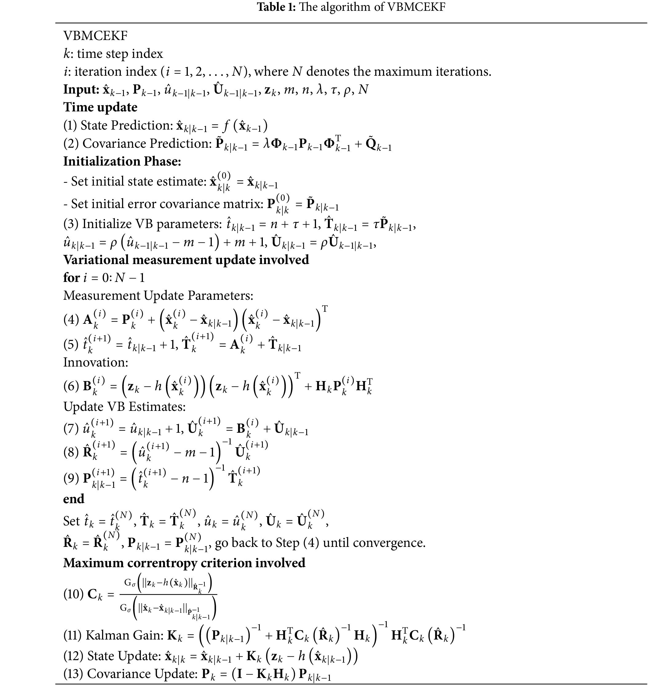
This update decreases the uncertainty in the state estimate by incorporating the latest measurement data, thus enhancing the accuracy of the predictions. The recursive approach for VBMCEKF, which is carried out based on Eqs. (18) to (38), is summarized in Table 1.

images

4 Results and Discussion

The current study uses a scenario for the positioning accuracies and error probability density functions are compared using four different methods including the extended Kalman filter (EKF), maximum correntropy extended Kalman filter (MCEKF), variational Bayesian extended Kalman filter (VBEKF), and variational Bayesian maximum correntropy extended Kalman filter (VBMCEKF). Additionally, the phenomena of multipath suppression are also considered. The simulated results are analyzed by using MATLAB software [23]. The Satellite Navigation (SatNav) Toolbox 3.0, a commercial software developed by GPSoft LLC, is used to design experimental data such as satellite location, speed, virtual distance, and virtual distance change rate. Eight visual satellites (red colour stars) are shown in Fig. 1, which displays their dispersion in the form of skyplot.

images

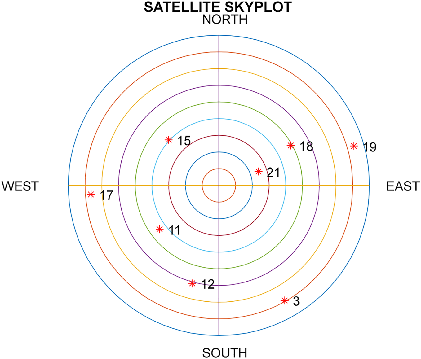
Figure 1: The skyplot

The proposed approach is investigated for a substantial effect in handling the time-varying measurement noise in an environment that includes both time-varying measurement noise and outliers. This is done to evaluate the properties of the filter. In two distinct noise scenarios, maximum correntropy is employed to mitigate outliers in time-varying observation noise simultaneously observed. The accuracy of the entire filter can then be increased while concurrently handling the issue of time-varying observation noise with outliers under a single filter structure. To replicate multipath situations, two periods of GPS observation data are combined with thermal noise of varied strengths. Ten outliers of varying strengths are added to each observation period to provide the time-varying magnitude of observation noise.

The study’s simulated motion trajectory, displayed in Fig. 2, is generated using the Satellite Navigation (SatNav) Toolbox 3.0 in MATLAB. This trajectory has a total journey duration of 639 s. Fig. 3 illustrates the additional interference sequences caused by outliers for the pseudorange observations. The simulation contains ten outliers, where the measurement inaccuracies could vary from a few tens to several hundred meters during the simulation process.

images

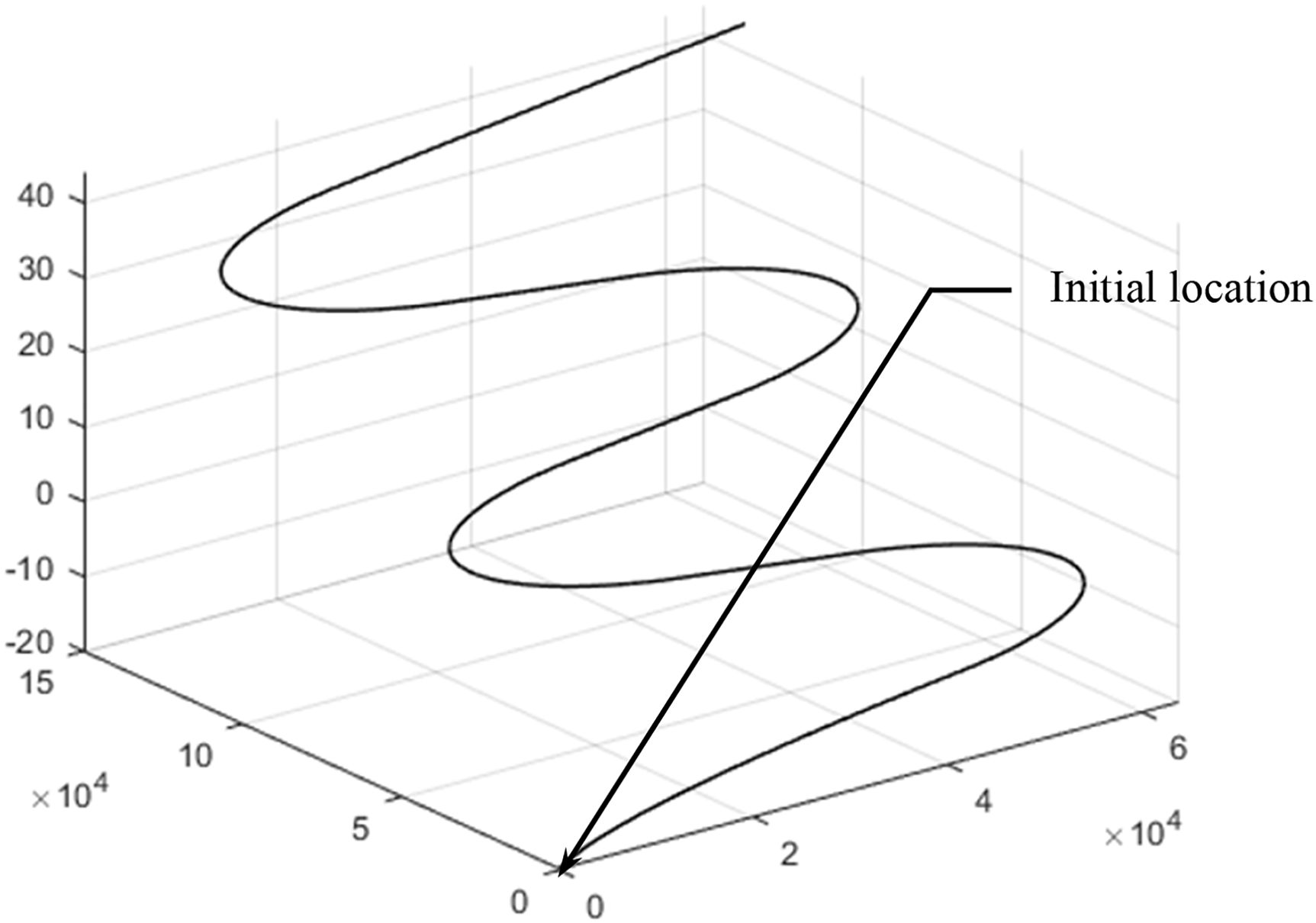
Figure 2: Test trajectory for the simulated vehicle

images

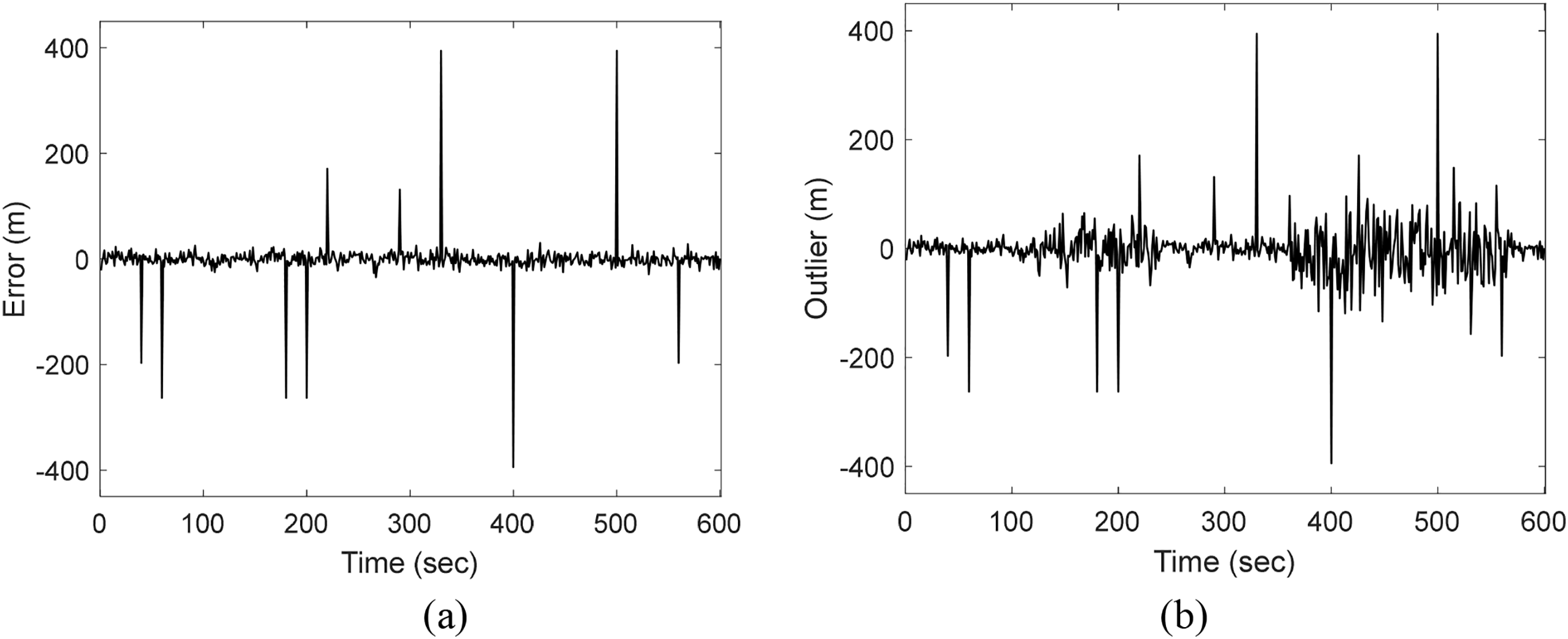
Figure 3: Data on sequences affected by outlier interferences

To simulate non-Gaussian noise in real-world conditions, we designed a simulation environment with time-varying observation noise. First, we simulated time-varying observation noise and applied it to two periods of GPS observation data. During these two periods, thermal noise of varying magnitudes was added to simulate the variation of noise in real environments. Secondly, we introduced 10 outliers of different magnitudes into each period to simulate the impact of multipath effects on positioning accuracy. Next, we will compare the performance of different filter algorithms, including EKF, VBEKF, MCEKF, and VBMCEKF. Through these performance comparisons, we can better evaluate how each algorithm performs in handling non-Gaussian noise environments.

Fig. 3a shows the sequence location diagram with added outlier interference, and (b) illustrates the simulation environment with two different periods and varying intensities of thermal noise and outlier interference sequences.

The kernel size in the VBMCEKF filter changes significantly over time, with multiple notable peaks throughout the process. Fig. 4 clearly illustrates this variation, showing how the kernel bandwidth ( $σ$ ) adapts dynamically over time. According to Eq. (18), the adaptive kernel bandwidth is calculated as $σμ,k=(||υμ,k(υμ,k)T||R^μ,k−1−1+Hμ,kPk|k−1HμT)$ . These peaks represent moments when the VBMCEKF filter reacts to sudden changes in the noise environment, such as increased noise intensity or the occurrence of outliers, prompting a rapid adjustment in the kernel size. This adaptive mechanism considers both the weighted innovation term and the weighted covariance of the estimation error, enabling the VBMCEKF to continuously optimize its noise-handling capabilities across different observation dimensions. This adaptive response enables the VBMCEKF to continuously optimize its noise handling capabilities, ensuring stability even under challenging noise conditions. The adaptability shown in Fig. 4 demonstrates the robustness of the VBMCEKF filter, allowing it to maintain effective filtering performance in real-world GNSS navigation scenarios with varying and unpredictable noise characteristics.

images

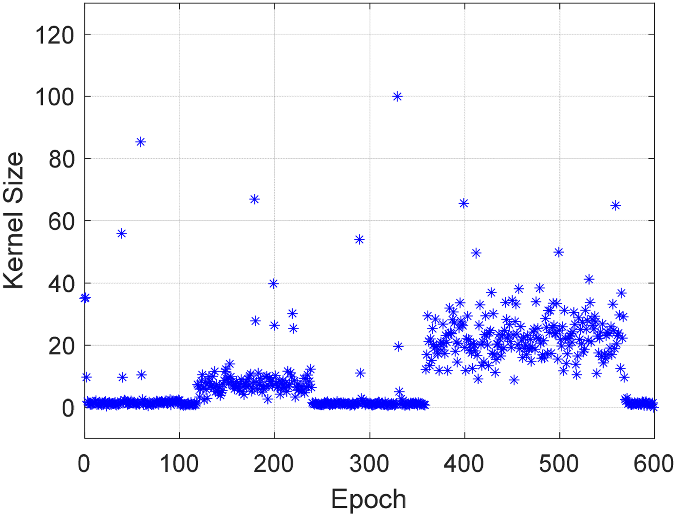
Figure 4: Adaptive kernel size variation over time in VBMCEKF

Fig. 5 illustrates the variation and adaptive capability of the standard deviation for time-varying statistics within the measurement model, highlighting its critical role in tracking the time-varying observation error covariance. As shown in Fig. 5, the results indicate that the adaptive performance of the VBMCEKF method surpasses that of both VBEKF and MCEKF, particularly in environments with high noise intensity. 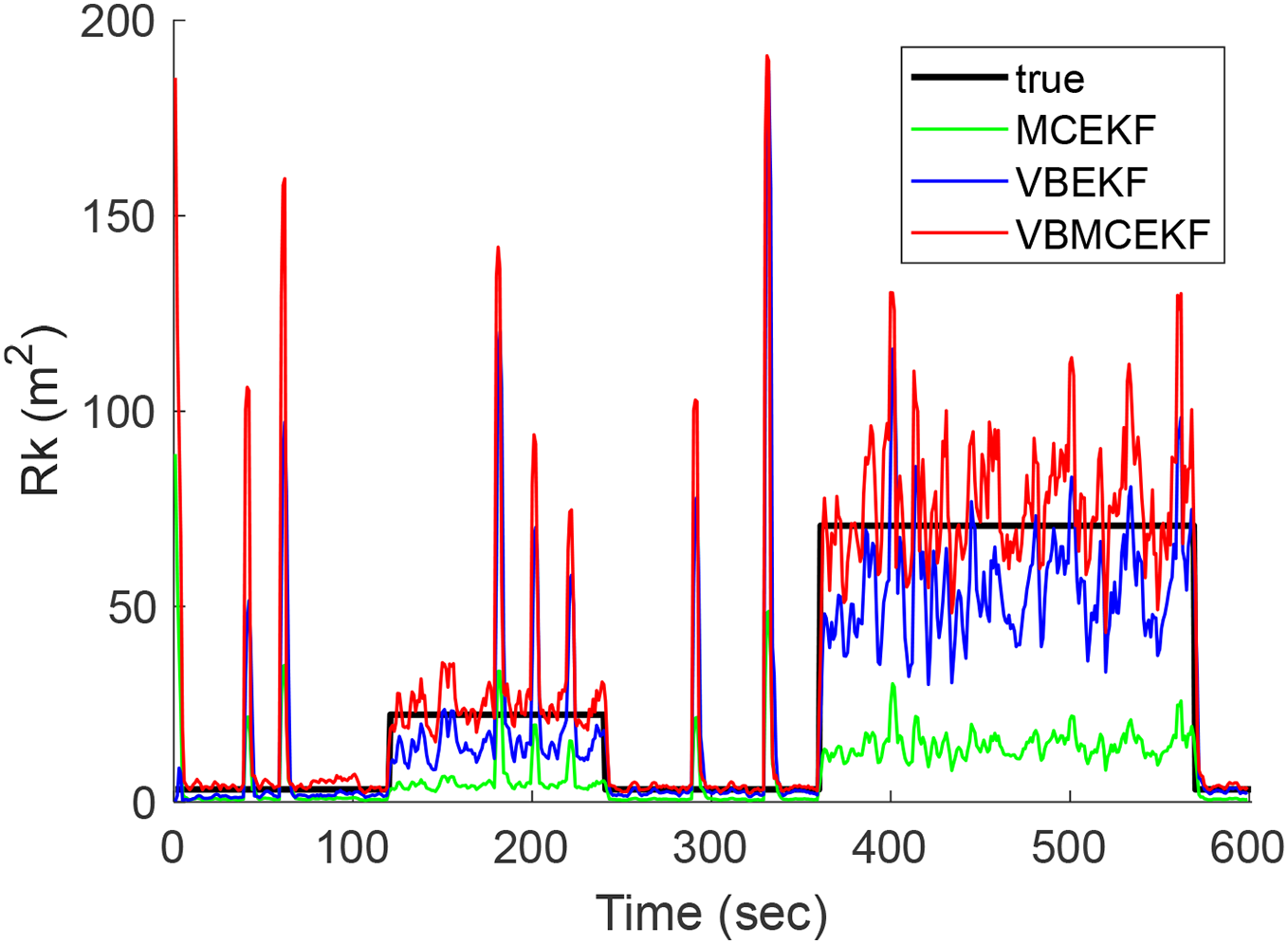Due to its lack of adaptive capability, the EKF was unable to track the variations in $Rk$ , thus limiting its effectiveness in handling non-stationary noise conditions. Similarly, the MCEKF struggled to capture the fluctuations in measurement noise strength. While the VBEKF was only marginally successful in tracking the variations in $Rk$ , the VBMCEKF, which integrates both the VB and MC mechanisms into the EKF framework, demonstrated superior adaptive capability, effectively tracking the measurement noise $Rk$ . With the incorporation of the VB mechanism, the VBMCEKF significantly enhances filter performance, improving its ability to adapt to challenging noise environments.

images

Figure 5: Variation and adaptation results of the variance for the time-varying measurement noise

In this simulation setup, we introduced 10 outliers of varying magnitudes distributed evenly across the time span to simulate the unpredictable interference often observed in real-world scenarios. Additionally, the thermal noise was divided into two distinct periods: one with higher intensity and one with lower intensity, designed to test the filter’s adaptability across different noise levels. These setups were intended to evaluate how well each filter responds to varying degrees of noise and outlier influence in a non-Gaussian environment. The results clearly demonstrate that VBMCEKF outperforms both VBEKF and MCEKF in handling these complex noise dynamics.

In this simulation, the bandwidth settings for the filters are defined as follows: the VBMCEKF employs an adaptive bandwidth that varies over time, while the MCEKF uses a fixed bandwidth denoted by $σ=3$ . A larger kernel bandwidth would cause MCEKF to behave similarly to the traditional EKF. Additionally, the initial parameters for the VBMCEKF are configured as follows: the time-scale parameter $τ$ is set to 10 × 1015, and the regularization parameter $ρ$ is set to 10 × 10−14. These parameter values were determined based on extensive GPS system simulation tests to ensure optimal performance. Such parameter settings allow the VBMCEKF to adapt effectively to non-Gaussian noise environments and ensure robust estimation performance, particularly under varying noise intensities.

In Fig. 6, the positioning errors in east, north, and altitude components have been analyzed in a comparison between the EKF and VBMCEKF. The VBMCEKF shows better suppression of outliers and slightly better adaptation to the time-varying strengths of thermal noise compared to the EKF. The outcome displays the positioning error probability density curves for the east, north, and altitude components, respectively. While the overall difference is not drastic, the VBMCEKF performs slightly better than the EKF, as evidenced by its probability density function, demonstrating a more concentrated distribution of errors with reduced heavy tails. This suggests that VBMCEKF provides more consistent and reliable estimates in the presence of thermal noise variations.

images

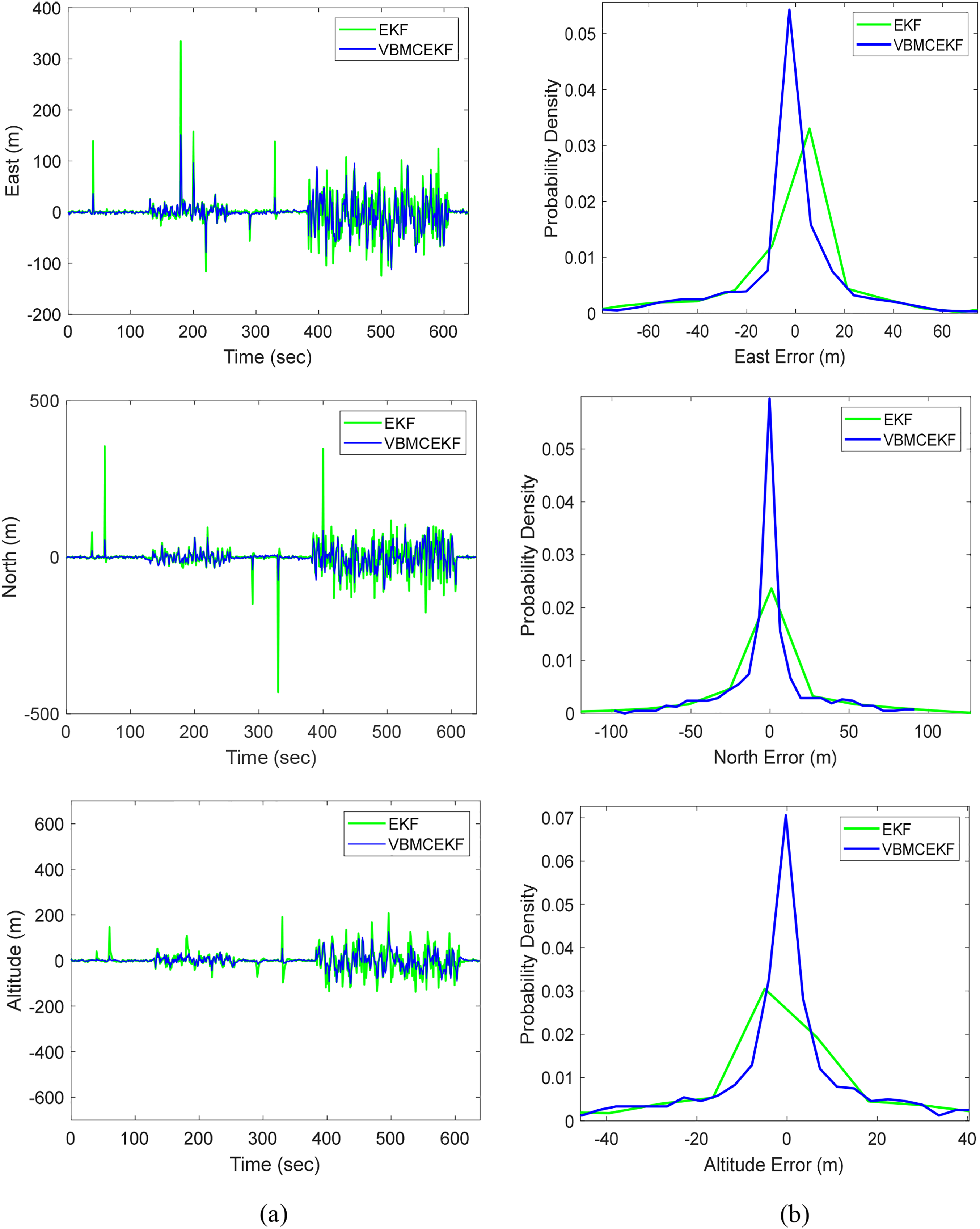
Figure 6: Comparison of positioning accuracy and the corresponding error probability density functions (pdf’s) for EKF and VBMCEKF: (a) Position errors; (b) probability density functions

Furthermore, the simulation results for east, north, and altitude positioning errors for EKF, VBEKF, MCEKF, and VBMCEKF were evaluated. The findings are shown in Fig. 7. Neither MCEKF nor VBEKF can suppress the outliers with sufficient accuracy. When compared to the other three filters, VBMCEKF shows a slight improvement in accuracy. While all filters have their respective strengths, VBMCEKF demonstrates more consistent performance, particularly in environments with varying noise intensities, providing somewhat better results in suppressing outliers and handling non-Gaussian noise.

images

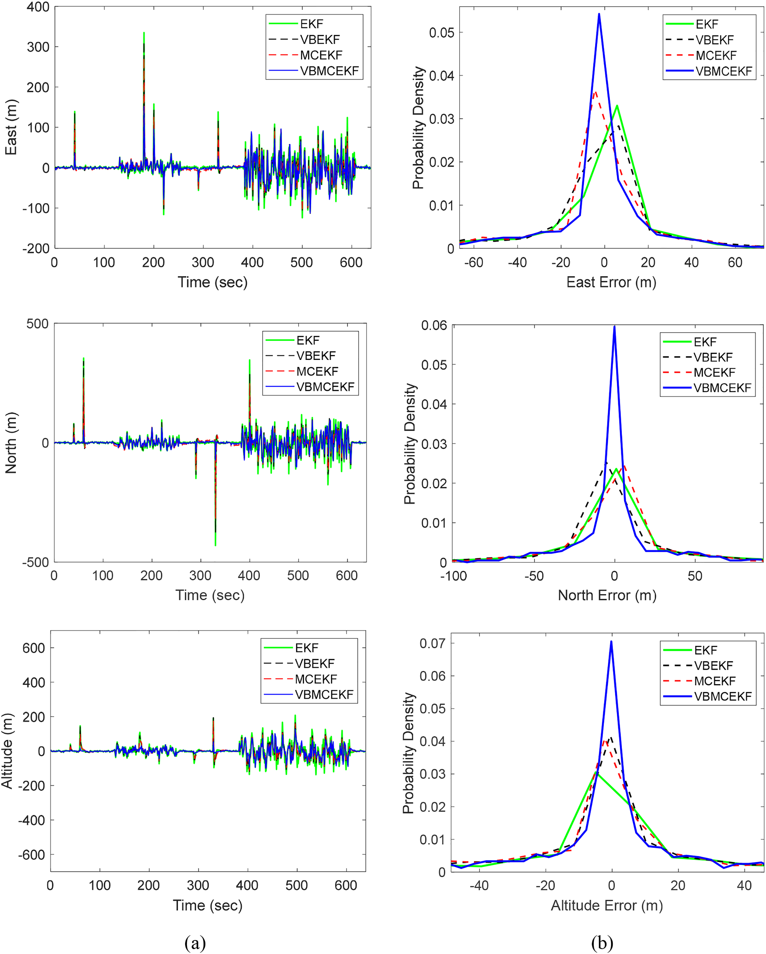
Figure 7: Comparison of positioning accuracy and the corresponding error probability density functions (pdf’s) for EKF, VBEKF, MCEKF and VBMCEKF: (a) Position errors; (b) probability density functions

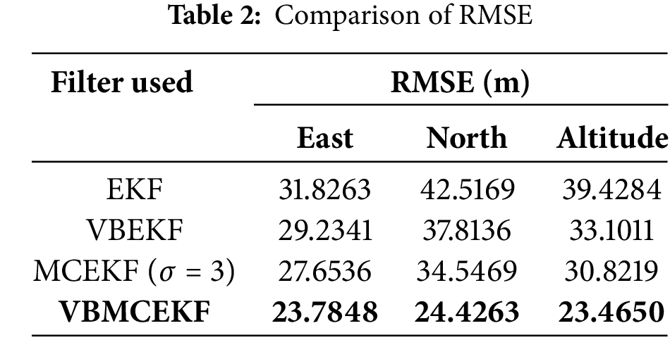
The quantitative performance comparison is presented in Table 2, which shows the root-mean-square error (RMSE) values for EKF, VBMCEKF, VBEKF, and MCEKF. The VBMCEKF achieves RMSE values of 23.7848, 24.4263, and 23.4650 m for the east, north, and altitude components, respectively. In contrast, EKF yields RMSE values of 31.8263, 42.5169, and 39.4284 m, while VBEKF and MCEKF perform slightly better than EKF but still inferior to VBMCEKF. These results demonstrate that VBMCEKF, with its combination of VB’s adaptive capability for measurement covariance filtering and MCC’s robustness in outlier suppression, significantly reduces error. It outperforms the other filtering methods, particularly in challenging carrier trajectory conditions.

images

5 Conclusions

This paper presents a novel integration of the Maximum Correntropy Criterion, variational Bayesian approach, and Extended Kalman Filter for improving GPS positioning and navigation accuracy in challenging noise environments. By estimating measurement noise with the variational Bayesian method and applying the Maximum Correntropy Criterion to handle outliers, this approach achieves both robustness and adaptability. To address potential filtering inaccuracies caused by inappropriate correntropy gain, an adaptive kernel bandwidth mechanism is introduced, ensuring precise tuning of the Maximum Correntropy Criterion-based Kalman filter. Additionally, the variational Bayesian method dynamically adjusts model parameters to handle time-varying noise, contributing to stable filtering performance.

This study presents significant advantages but is not without limitations. First, the adaptive kernel bandwidth mechanism, while effective for handling time-varying noise, can be computationally demanding, making it less suitable for systems with strict resource or real-time constraints. Second, the evaluation of the proposed method has been largely limited to simulated non-Gaussian noise conditions, requiring additional testing to verify its performance in complex real-world scenarios with mixed noise types. Lastly, the approach relies heavily on accurate initial parameter estimation, which can undermine its robustness when prior information is incomplete or unreliable.

In non-Gaussian environments, the Maximum Correntropy Criterion effectively mitigates ambient noise effects through dynamic kernel bandwidth adjustment, which is particularly beneficial in complex, time-varying scenarios. When combined with the Extended Kalman Filter, this approach significantly enhances system robustness and improves state estimation accuracy, minimizing the adverse effects of outliers and noise on GPS navigation results. Experimental results confirm that the proposed method outperforms traditional approaches by maintaining stable filtering performance and reducing noise impacts across various non-Gaussian noise conditions. Although certain limitations remain, this work demonstrates strong potential for real-world global navigation satellite system applications requiring high precision in unpredictable, noise-heavy environments.

Acknowledgement: The authors gratefully acknowledge the financial support from the National Science and Technology Council.

Funding Statement: This work has been partially supported by the National Science and Technology Council, Taiwan under grants NSTC 111-2221-E-019-047 and NSTC 112-2221-E-019-030.

Author Contributions: The authors confirm contribution to the paper as follows: guidance and oversight throughout the project: Dah-Jing Jwo; study conception and design: Dah-Jing Jwo; data collection: Yi Chang; analysis and interpretation of results: Dah-Jing Jwo, Ta-Shun Cho; experimental design and perform data analysis: Dah-Jing Jwo, Yi Chang, Ta-Shun Cho; draft manuscript preparation: Dah-Jing Jwo, Yi Chang, Ta-Shun Cho. All authors reviewed the results and approved the final version of the manuscript.

Availability of Data and Materials: The data and related programs are available from the corresponding authors upon reasonable request.

Ethics Approval: Not applicable.

Conflicts of Interest: The authors declare no conflicts of interest to report regarding the present study.

References

1. Kaplan ED. Understanding GPS: principles and applications. 2nd ed. Boston: Artech House Publishers; 1996. [Google Scholar]

2. Singh A, Principe JC. Using correntropy as a cost function in linear adaptive filters. In: IEEE Proceedings of the International Joint Conference on Neural Networks (IJCNN); 2009; Atlanta, GA, USA. p. 2950–5. [Google Scholar]

3. Zou Y, Zou S, Tang X, Yu L. Maximum correntropy criterion Kalman filter based target tracking with state constraints. In: Proceedings of the 39th Chinese Control Conference (CCC); 2020 Jul 27–29; Shenyang, China. p. 3505–10. [Google Scholar]

4. Liu X, Qu H, Zhao J, Chen B. Extended Kalman filter under maximum correntropy. In: IEEE Proceedings of the 2016 International Joint Conference on Neural Networks; 2016; Vancouver, BC, Canada. p. 1733–7. [Google Scholar]

5. Wang G, Li N, Zhang T. Maximum correntropy unscented Kalman and information filters for non-Gaussian measurement noise. J Franklin Inst. 2017;354(18):8659–77. doi:10.1016/j.jfranklin.2017.10.023. [Google Scholar] [CrossRef]

6. Brown RG, Hwang PYC. Introduction to random signals and applied kalman filtering. New York, NY, USA: John Wiley and Sons; 1997. [Google Scholar]

7. Jwo DJ, Chang SJ. Outlier resistance estimator for GPS positioning. In: IEEE International Conference on Systems, Man, and Cybernetics; 2006; Taipei, Taiwan. [Google Scholar]

8. Fan X, Wang G, Han J, Wang Y. A background-impulse kalman filter with non-gaussian measurement noises. IEEE Transact Syst, Man Cyberne: Syst. 2023;53(4):2434–43. doi:10.1109/TSMC.2022.3212975. [Google Scholar] [CrossRef]

9. Chen B, Dang L, Gu Y, Zheng N, Principe JC. Minimum error entropy Kalman filter. IEEE Transact Syst, Man Cyberne: Syst. 2019;51(9):5819–29. doi:10.1109/TSMC.2019.2957269. [Google Scholar] [CrossRef]

10. Liu WF, Pokharel PP, Principe JC. Correntropy: properties and applications in non-Gaussian signal processing. IEEE Transact Signal Process. 2007;55(11):5286–98. doi:10.1109/TSP.2007.896065. [Google Scholar] [CrossRef]

11. Zhao S, Chen B, Principe JC. Kernel adaptive filtering with maximum correntropy criterion. In: IEEE Proceedings of the International Joint Conference on Neural Networks (IJCNN); 2011; San Jose, CA, USA. p. 2012–7. [Google Scholar]

12. Wang Y, Lu Y, Zhou Y, Zhao Z. Maximum correntropy criterion-based UKF for loosely coupling INS and UWB in Indoor localization. Comput Model Eng Sci. 2024;139(3):2673–793. doi:10.32604/cmes.2023.046743. [Google Scholar] [CrossRef]

13. Attias H. A variational Bayesian framework for graphical models. In: Advances in neural information processing systems. Cambridge, MA, USA: MIT Press; 2000. [Google Scholar]

14. Beal MJ. Variational algorithms for approximate Bayesian inference [Ph.D. thesis]. UK: University of London; 2003. [Google Scholar]

15. Li K, Chang L, Hu B. A variational Bayesian-based unscented Kalman filter with both adaptivity and robustness. IEEE Sens J. 2016;16(18):6966–76. doi:10.1109/JSEN.2016.2591260. [Google Scholar] [CrossRef]

16. Liu X, Liu X, Yang Y. Variational Bayesian-based robust cubature Kalman filter with application on SINS/GPS integrated navigation system. IEEE Sens J. 2022;22(1):489–500. doi:10.1109/JSEN.2021.3127191. [Google Scholar] [CrossRef]

17. Chen B, Liu X, Zhao H, Principe JC. Maximum correntropy Kalman filter. Automatica. 2017;76:70–7. doi:10.1016/j.automatica.2016.10.004. [Google Scholar] [CrossRef]

18. Fan Y, Zhang Y, Wang G, Wang X, Li N. Maximum correntropy based unscented particle filter for cooperative navigation with heavy-tailed measurement noises. Sensors. 2018;18(10):3183. doi:10.3390/s18103183. [Google Scholar] [PubMed] [CrossRef]

19. Wang G, Gao Z, Zhang Y, Ma B. Adaptive maximum correntropy Gaussian filter based on variational Bayes. Sensors. 2018;18(6):1960. doi:10.3390/s18061960. [Google Scholar] [PubMed] [CrossRef]

20. He J, Sun C, Zhang B, Wang P. Variational Bayesian-based maximum correntropy cubature Kalman filter with both adaptivity and robustness. IEEE Sens J. 2020;21(2):1982–92. doi:10.1109/JSEN.2020.3020273. [Google Scholar] [CrossRef]

21. Izanloo R, Fakoorian SA, Yazdi HS, Simon D. Kalman filtering based on the maximum correntropy criterion in the presence of non-Gaussian noise. In: IEEE Proceedings of the 2016 Annual Conference on Information Science and Systems (CISS); 2016; Princeton, NJ, USA. [Google Scholar]

22. Huang Y, Bai M, Li Y, Zhang Y, Chambers J. An improved variational adaptive Kalman filter for cooperative localization. IEEE Sens J. 2021;21(9):10775–86. doi:10.1109/JSEN.2021.3056207. [Google Scholar] [CrossRef]

23. Huang B, Wang J, Zhang J, Yu D, Feng P. Variational Bayesian adaptive Kalman filter for integrated navigation with unknown process noise covariance. In: IEEE Proceedings of the 2022 2nd International Conference on Consumer Electronics and Computer Engineering (ICCECE); 2022; Guangzhou, China. [Google Scholar]

24. Qiao S, Wang G, Fan Y, Mu D, He Z. A novel adaptive maximum correntropy criterion Kalman filter based on variational Bayesian. In: IEEE Proceedings of the 2022 34th Chinese Control and Decision Conference (CCDC); 2022; Hefei, China. [Google Scholar]

25. Qiao S, Fan Y, Wang G, Mu D, He Z. Maximum correntropy criterion variational Bayesian adaptive Kalman filter based on strong tracking with unknown noise covariances. J Franklin Inst. 2023;360(9):6515–36. doi:10.1016/j.jfranklin.2023.04.015. [Google Scholar] [CrossRef]

26. GPSoft LLC. Satellite Navigation (SatNav) Toolbox 3.0 user’s guide. Athens, OH, USA: GPSoft LLC; 2003. [Google Scholar]

Cite This Article

APA Style

Jwo, D., Chang, Y., Cho, T. (2025). A robust GNSS navigation filter based on maximum correntropy criterion with variational bayesian for adaptivity. Computer Modeling in Engineering & Sciences, 142(3), 2771–2789. https://doi.org/10.32604/cmes.2025.057825

Vancouver Style

Jwo D, Chang Y, Cho T. A robust GNSS navigation filter based on maximum correntropy criterion with variational bayesian for adaptivity. Comput Model Eng Sci. 2025;142(3):2771–2789. https://doi.org/10.32604/cmes.2025.057825

IEEE Style

D. Jwo, Y. Chang, and T. Cho, “A Robust GNSS Navigation Filter Based on Maximum Correntropy Criterion with Variational Bayesian for Adaptivity,” Comput. Model. Eng. Sci., vol. 142, no. 3, pp. 2771–2789, 2025. https://doi.org/10.32604/cmes.2025.057825

BibTex EndNote RIS

Copyright © 2025 The Author(s). Published by Tech Science Press.
This work is licensed under a Creative Commons Attribution 4.0 International License , which permits unrestricted use, distribution, and reproduction in any medium, provided the original work is properly cited.

Table of Content

A Robust GNSS Navigation Filter Based on Maximum Correntropy Criterion with Variational Bayesian for Adaptivity

Abstract

Keywords

References

Cite This Article

466

197

0

Related articles

Further Information

Guidelines

Follow Us

Join Us

Share Link