
 Submit a Paper
 Propose a Special lssue
 Open Access
ARTICLE

A Geometric Model Simplification Strategy for CFD Simulation of the Cockpit Internal Environment
1 Tianjin Key Lab. of Indoor Air Environmental Quality Control, School of Environmental Science and Engineering, Tianjin University, Tianjin, 300072, China
2 Architectural Institute, China Railway Design Corporation, Tianjin, 300308, China
3 Environmental Control Oxygen Department, Shanghai Aircraft Design and Research Institute, COMAC, Shanghai, 201210, China
* Corresponding Author: Zhengwei Long. Email:
Computer Modeling in Engineering & Sciences 2025, 142(2), 1545-1564. https://doi.org/10.32604/cmes.2025.058773
Received 20 September 2024; Accepted 20 December 2024; Issue published 27 January 2025
 View Full Text
 Download PDF
Abstract
Computational Fluids Dynamics (CFD) simulations are essential for optimizing the design of a cockpit’s internal environment, but the complex geometric models consume a significant amount of computational resources and time. Arbitrary simplification of geometric models may result in inaccurate calculations of physical fields. To address this issue, this study establishes a geometric model simplification strategy and successfully applies it to a cockpit. The implementation of the whole approach is divided into three steps, summarized in three methods, namely Sensitivity Analysis Method (SAM), Detail Suppression Method (DSM), and Evaluation Standards Method (ESM). Sensitivity analysis of the detailed features of the geometric model is performed using the adjoint method. The details of the geometric model are suppressed based on the principle of curvature continuity. After evaluation, the suppression degrees of detailed features with different sensitivity levels are obtained. The results demonstrate that this strategy can be employed to achieve precise simplification standards, thereby avoiding excessive deviations caused by arbitrary simplification and reducing the significant costs associated with trial-and-error simplification.Keywords
Computational Fluid Dynamics (CFD) is a numerical method of simulating and analyzing fluid dynamics in an aircraft cabin by solving the governing equations using computers [1–5]. It is one of the best alternative methods to expensive and time-consuming experimental studies [6–9]. Its main work process includes three stages: pre-processing, solution calculation, and post-processing [10]. Among them, pre-processing is the foundation of the entire simulation analysis, mainly including two parts: model idealization and grid generation [10–12]. A large number of detailed features in the cockpit can greatly increase the complexity of grid generation and solving calculations [13–14], and even lead to grid generation failure or incorrect simulation results [15–16]. Therefore, model simplification is a necessary step [17], especially in studies focused on optimizing internal air supply schemes, where hundreds or thousands of case calculations are usually required, hence the initial geometric model simplification can reduce substantial computational time and cost [18–19]. Researchers choose to delete or partially delete detailed features of the interior surface [20–24] and simplify curved surfaces to planes [21,25–27]. In some studies, the dummy model is simplified to a block dummy instead of a model with a human body shape [20,28–30]. Cao et al. [29] established a seven-row cabin model and evaluated the impact of removing seat legs on the accuracy of cabin airflow field prediction. It was found that removing only seat legs can save nearly one million grid cells and shorten calculation time by 20%. Despite these studies simplifying geometric models, there is no clear basis for the simplification process [31–34]. The absence of a simplification basis may result in deviations in solving physical fields and substantial trial-and-error costs during the arbitrary simplification process until a simplification that corresponds to experimental results is found. Model simplification methods have made some progress in the field of CAD [16], but these methods are essentially directly or indirectly based on the geometric properties of the model, without considering the physical environment in which the model is located, making it difficult to ensure simulation accuracy [35]. Therefore, it is crucial to propose an integrated geometric model simplification strategy based on the physical environment to ensure a balance between simulation efficiency and accuracy. It means taking specific research questions and key physical parameters as the background. In other words, for the same geometric model, there should be different simplified forms in different research questions to enhance its adaptability. It is thus necessary to explore the sensitivity of geometric boundaries regarding the studied problems. Suresh and his collaborators first studied the issue of the impact of removing a single feature on the accuracy of engineering simulations [36–39], using the concept of “feature sensitivity” to define the feature suppression error. The feature suppression error mainly studies the impact of removing tiny features on the accuracy of engineering simulations, which is closely related to the shape sensitivity analysis (SSA) [40]. SSA is defined as the differential of the physical objective function on the geometric model with respect to the shape parameters of the features. For example, Taroco et al. [40] proposed a method for solving second-order shape sensitivity analysis in non-linear problems. Antolín et al. [41] proposed a posteriori error estimator to evaluate the errors caused by removing Neumann features and to determine the influence of different features on the calculation results. In Huang’s research, the adjoint solver was utilized for sensitivity analysis, and the quasi-Newton optimization solver was adopted for shape optimization, which improved the aeroelastic characteristics [42]. In Liu’s research [43], the adjoint equation was used for sensitivity analysis to guide the shape optimization of the pore structure, effectively improving the radiative heat absorption efficiency. In Tang’s research [44], by analyzing the adjoint sensitivity distribution, it was determined that the regions near the middle of the suction surface and the leading edge had the greatest impact on the aerodynamic performance. These studies have demonstrated that the adjoint solver is an efficient tool for conducting sensitivity analysis. Therefore, in the simplification of geometric models, the adjoint method can also be used for sensitivity analysis to determine the impact of detailed features on the physical field.
This study develops a strategy for simplifying geometric models in cockpit simulations, aiming to address three issues, namely, where to simplify, how to simplify, and to what extent to simplify. Sensitivity Analysis Method (SAM), Detail Suppression Method (DSM) and Evaluation Standards Method (ESM) are proposed in this strategy, which can guide the simplification of geometric models. The effectiveness of the geometric model simplification strategy has been verified on an aircraft cockpit. It is worth noting that the study provides a geometric model simplification strategy, not a uniform simplification standard that is directly applicable to all different cockpit models, as different cockpit models have their unique detailed features.
This study proposes a simplification strategy for the detailed features in the model, which includes Sensitivity Analysis Method (SAM), Detail Suppression Method (DSM) and Evaluation Standards Method (ESM), as shown in Fig. 1.
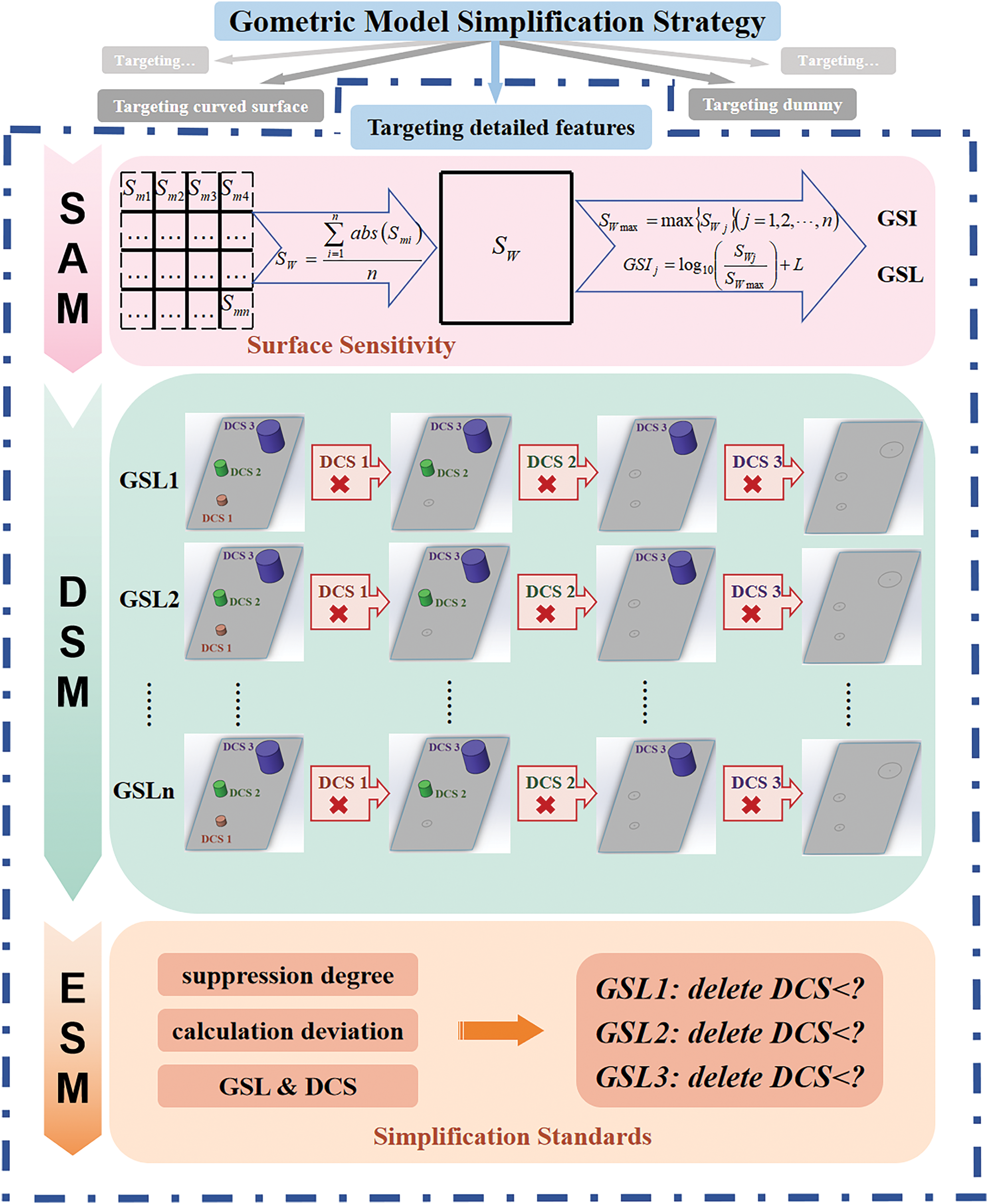
Figure 1: Methodology roadmap of the geometric model simplification strategy
2.1 Sensitivity Analysis Method (SAM)
The derivative of the target parameters with respect to the geometric surface offset is defined as the Sensitivity. Solving for sensitivity using the adjoint method. There are two main equations in the formulation of the adjoint method. The first equation is the residual form of the Navier-Stokes (N-S) equation, and the second one is the cost function, which are related to shape variables
The derivatives of above two equations can be represented as shown in Eqs. (3) and (4).
Eq. (5) is obtained from Eq. (3).
Putting the Eq. (5) in Eq. (4), the sensitivity can be represented as shown in Eq. (6).
To consider the constraint by the NS equation,
By putting the value of
The above sensitivity solution results, based on mathematical principles, calculate the sensitivity of each grid cell. Denote the sensitivity
where
2.1.2 Geometric Sensitivity Index (GSI) and Geometric Sensitivity Level (GSL)
This paper proposes the concept of Geometric Sensitivity Index (GSI) and Geometric Sensitivity Level (GSL), with the physical meaning of analyzing the sensitivity of each detailed feature. The specific calculation method is as follows:
The comprehensive
When making overall changes to the geometric surface, the impact on the target cost function is the coupling effect of all grid offsets. Therefore, the significance of using its absolute value as a reference for quantitative analysis of geometric sensitivity is relatively low. The Geometric Sensitivity Level (GSL) is used to divide the sensitivity level. The larger the GSI, the higher the GSL, and the greater the impact on the cost function from geometric model changes. In this study, the GSL of the cockpit surface is divided into three levels, that is
The Sensitivity Analysis Method (SAM) is implemented based on the adjoint method in STAR-CCM+ 2020.3.1, and the specific steps are as follows:
(1) Establish geometric models and set boundary conditions;
(2) Using a coupled solver to solve physical fields;
(3) Activate the adjoint solver;
(4) Define cost function;
(5) Calculate Surface Sensitivity (
(6) Calculate the GSI and GSL of each surface.
2.2 Detail Suppression Method (DSM)
The Detail Suppression Method, as the name suggests, is to suppress the detailed features that have less influence on the physical field. Since detailed features are surrounded by surfaces, suppressing features is achieved by deleting surfaces [16], which can lead to surface voids and co-surface loops. A co-surface loop is a boundary loop on the same underlying surface [47]. A new surface is constructed with the co-surface loop as the boundary to close the void in the original model. Ensuring the curvature of the new surface’s boundary matches that of the underlying surface on the ring allows for a natural and smooth connection [48]. Subsequently, the new surface is finally sewn with the underlying surface to make it an integral part of the model, ensuring that the final simplified model is close to the original model.
Due to the complexity and diversity of the detailed features inside the cockpit, the size of these features should not only depend on their absolute size, but also on the relative size to the surface they are located on. Therefore, defining Dimensionless Characteristic Size (DCS) to measure the relative size of detailed features:
where
Based on the results of the SAM, all the detailed features are classified into different categories according to the GSL. The higher the GSL of a detailed feature is, the greater the impact its change will have on the physical field. The suppression degree is defined as the maximum DCS value of the suppressed detailed features. During the DSM exploration process, the suppression degree of each category is gradually increased to create different simplified versions, and their physical fields are calculated through CFD simulations. In the subsequent ESM process, the physical field deviations resulting from simplification would be calculated for each version and the simplification standard could be obtained.
2.3 Evaluation Standards Method (ESM)
For simulating buildings, cabins, and other human settlement environments, the key focus is on the air state around the human body, and the key physical quantities are air temperature and velocity. Therefore, several points can be taken on the target area to compare and calculate the absolute and relative deviations of temperature and velocity before and after simplification. The calculation equations for absolute deviation and relative deviation are as follows:
where
Simulation results of each version are obtained in the DSM, and the deviation calculations are carried out through Eqs. (17) and (18). Based on different GSL categories, the result deviation is fitted with the suppression degree to obtain the relationship between the two. The simplification strategy should determine the maximum suppression degree for each GSL category of detail features based on the acceptable deviation.
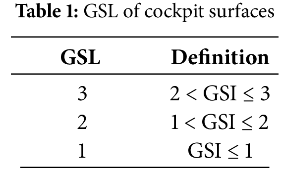
A cockpit was chosen as the object of study because the interior of the cockpit has more detailed features compared to the passenger cabin, and the application of this geometric simplification strategy is more representative. The cockpit was equipped with a pilot’s seat, a copilot’s seat, and two observers’ seats. There was a central console between the pilots and five monitors on the internal instrument panel. A glare shield was set above the monitors. Counters and side consoles were also set on the left and right sides. A top air inlet was located in the center of the ceiling. The main air inlets, shoulder air inlets, foot air inlets, and front windshield air inlets were symmetrically positioned on both left and right sides. A foot return air outlet was symmetrically positioned on the side wall surface near the floor. The computational domain and vent position can be seen in Fig. 2.
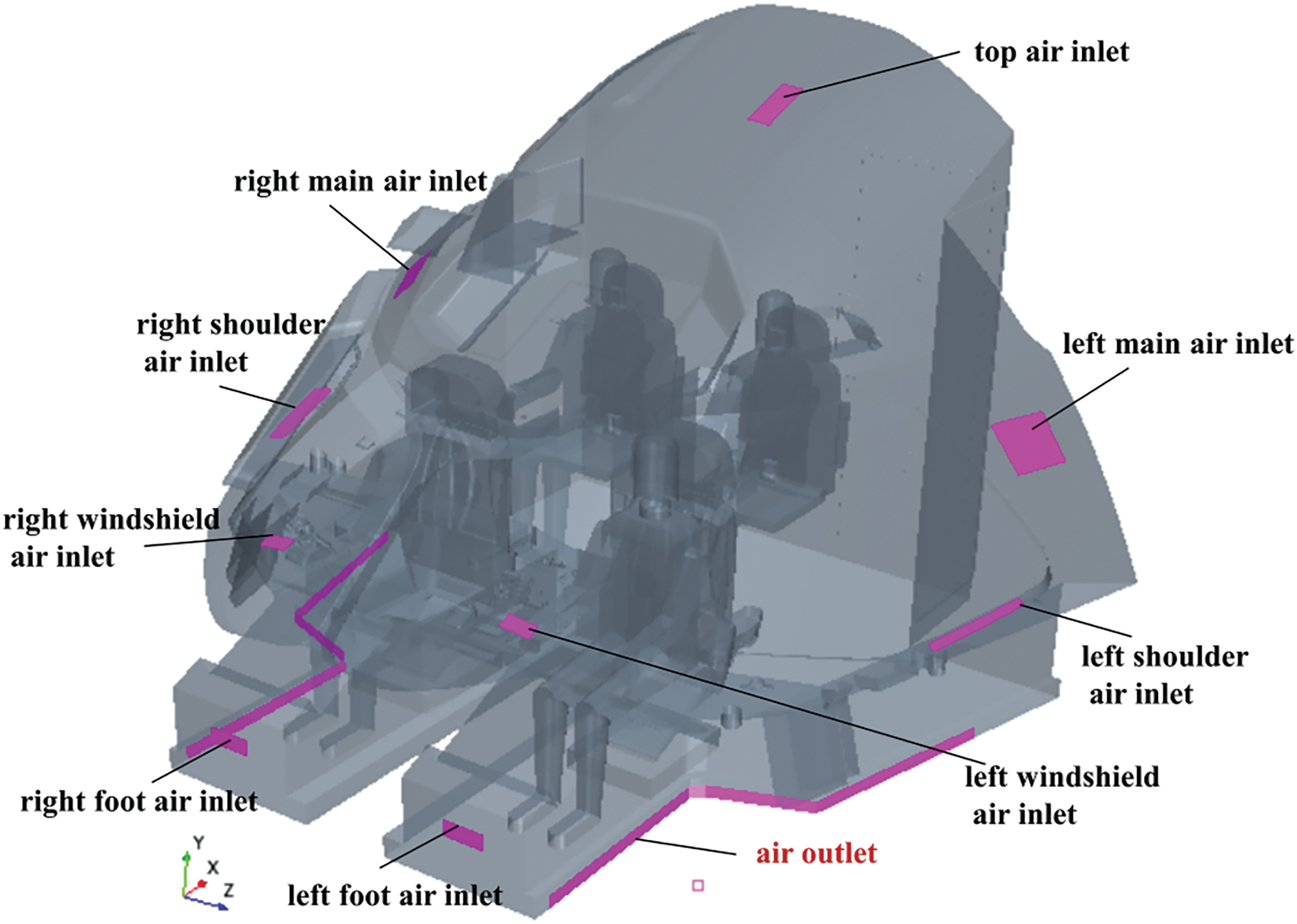
Figure 2: Computational domain and vents position of the cockpit
3.2 Physical Model and Boundary Conditions
The airflow field in the cockpit domain was solved using the incompressible Navier-Stokes (N-S) equation. Reynolds-Averaged Navier-Stokes (RANS) method was used to simulate turbulence, as the RANS numerical calculation method has been widely applied in engineering fields [49–51]. Based on previous research into the simulation of aircraft cabin environments, the Realizable k-ε turbulence model was used to be closest to the experimental data [29,52]. The aircraft cabin airflow can be considered as a low-velocity incompressible flow and the density is considered to be constant, therefore, the Boussinesq approximation was used to account for the buoyancy effect [53–56]. The discrete method adopted the finite volume method, and the second-order upwind scheme was utilized to discrete the turbulent kinetic energy, dissipation rate, and momentum to attain better robustness of the results.
The walls were divided into convective boundary, temperature boundary and adiabatic boundary, according to the characteristics of the components in the cockpit. The mass flow rates for the top air inlet, shoulder air inlet, foot air inlet, windshield air inlet, and main air inlet were 0.0236, 0.0236, 0.0034, 0.0076 and 0.380 kg/s respectively. All air supply temperatures were 16°C.
3.3 Grid Configuration and Independence Test
Because of the complexity of the cockpit geometry model, the polyhedral mesh was selected to discretize the entire computational domain. Compared to the widely utilized tetrahedral mesh, polyhedral meshes have shown superior performance while discretizing these geometries with complex features [26]. The base size of grid cells was set to 30 mm, while the size was reduced to 10 mm around personnel and air inlets and outlets, where there was a large velocity or temperature gradient [12]. To accurately capture the detailed gradient changes of the important parameter (e.g., velocity) near the dummy surface and wall, the Prism Layer Mesher was used to divide the boundary layer to four prism layers with a first layer height of 1.23 mm.
To conserve computational resources, the grid independence test was performed on model V6 (V6 simplification presented in Section 4.2). Based on the structural characteristics of the cockpit and existing computing capabilities, three sets of grids with numbers of 1.53, 2.96, and 6.71 million were performed. A line on the cross-section of the cockpit was selected to compare the velocity field distribution, as shown in Fig. 3. The results with 2.96 million cells were nearly the same as those with 6.71 million cells, but there was an obvious deviation between the 1.53 and 2.96 million cells. Therefore, the 2.96-million-cell grid was selected for subsequent calculations.
Figure 3: Results of grid independence test
Also, according to the simplified model V6 (V6 simplification presented in Section 4.2), an experimental platform was built with the same dimensions as the real cockpit in full scale, as shown in Fig. 4. To verify the accuracy of simulations, comparison between the experiment and simulation was conducted. Temperatures and velocities on two typical lines (L1 and L2) were selected. The height of L1 and L2 was 1.1 m, located in front of pilots and observers respectively. According to the simulation results, it is initially judged that the temperature range of the measurement point is 17°C–20°C and the velocity is less than 1 m/s, so Hot-wire Anemometers Testo 405i were applied to measure the temperature and velocity distribution. The measurable range of temperature is −20°C–60°C with an accuracy of ±0.5°C. The measurable range of speed is 0–30 m/s, with an accuracy of ± (0.1 m/s + 5% of the measured value) within the 0–2 m/s measuring range. As shown in Fig. 5, the maximum error of temperature results between simulation and experiment is 5.6%, and the maximum error of velocity is 0.09 m/s, indicating good agreement between experimental and numerical results.
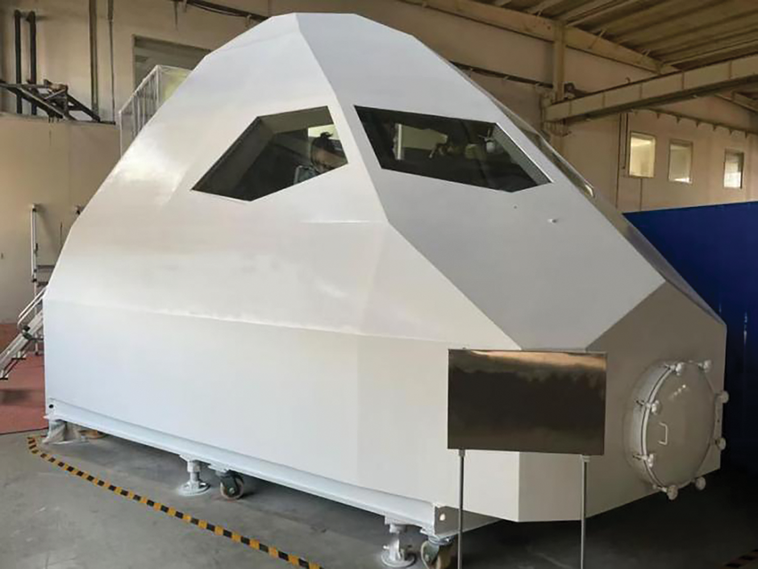
Figure 4: The cockpit experimental platform in full scale
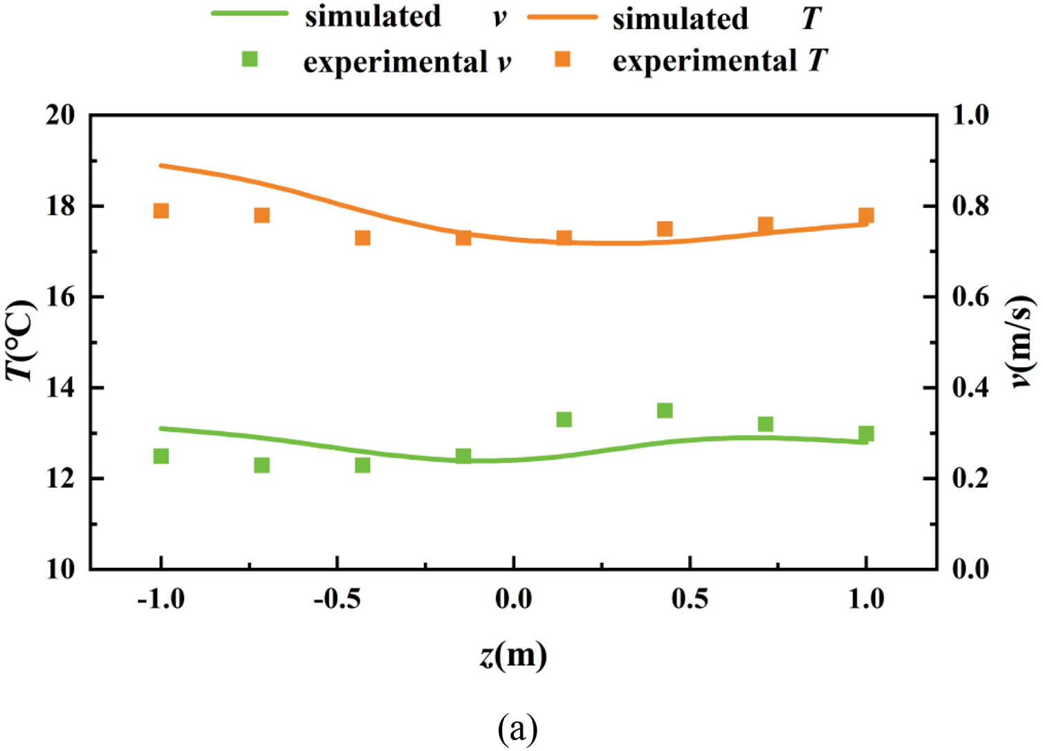
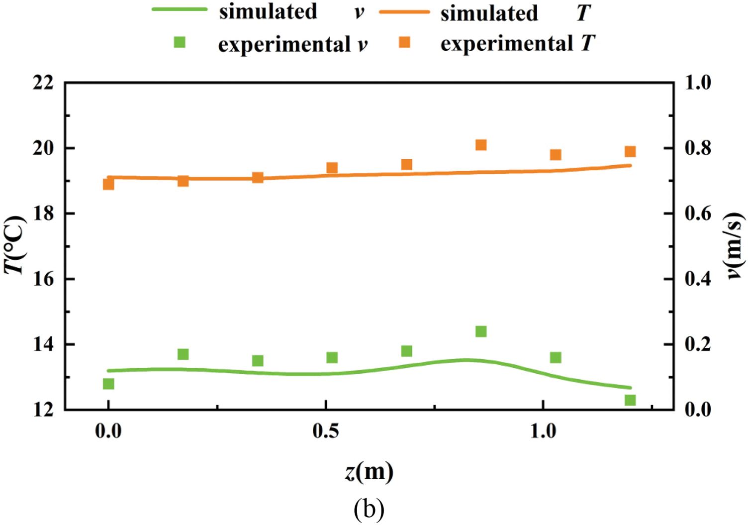
Figure 5: Comparison of the temperature and velocity distributions on (a) L1; (b)L2
4.1 Sensitivity Evaluation through SAM
Cost functions are established based on the front and side regions of the pilots and observers (the yellow region in Fig. 6) as follows:
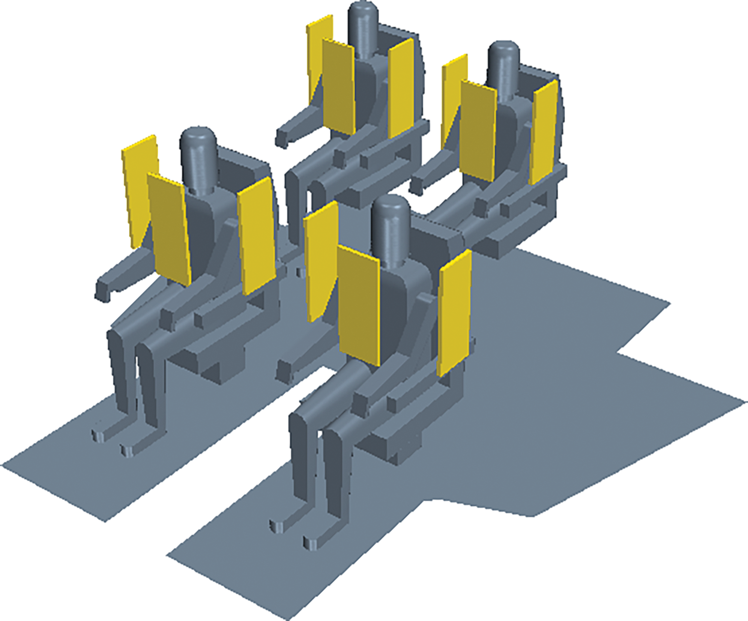
Figure 6: Focused region by sensitivity analysis
where
where
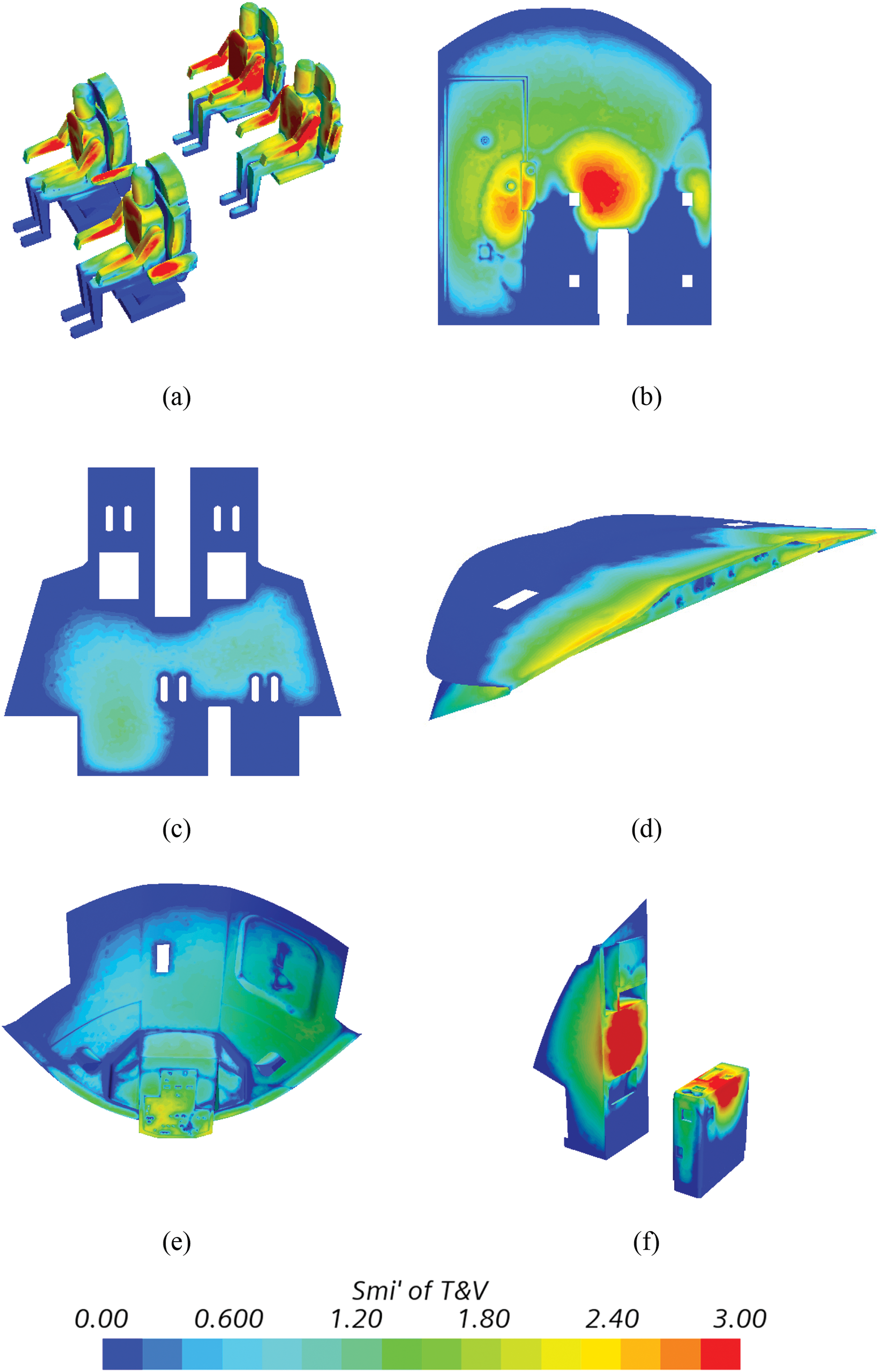
Figure 7:
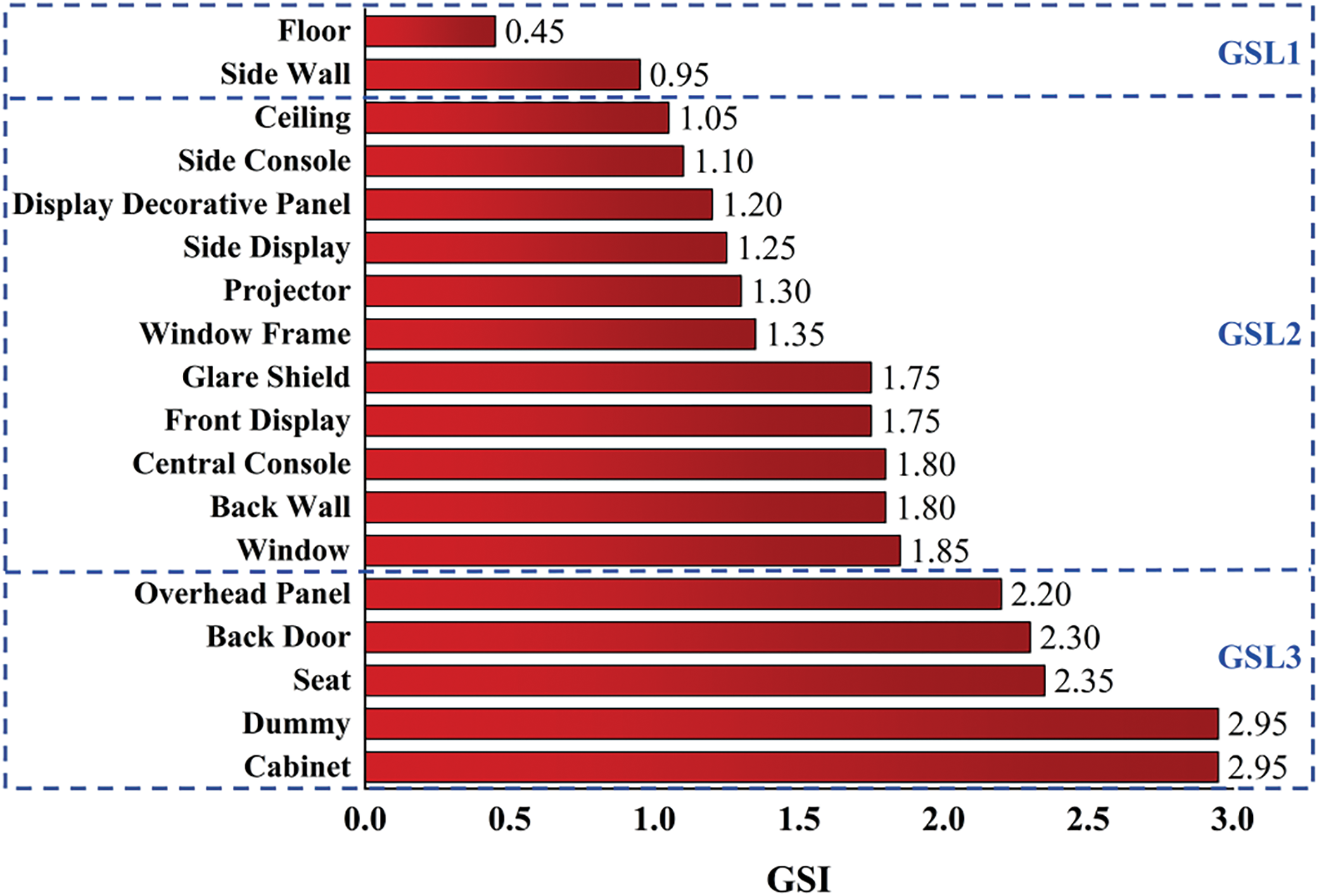
Figure 8: GSI results of walls in the cockpit
Analyzing the sensitivity results of various surfaces in the cockpit, cabinets, dummies, and seats are the most sensitive areas. It can be observed that the sensitivity of surfaces closer to the focused area is usually higher, including the overhead panel, windows, front displays, and glare shields. This observation aligns with our expectations and supports the accuracy of the sensitivity analysis. Therefore, when using SAM to study the geometric sensitivity of the model, the focused region should be determined first, and usually, the region close to the personnel is selected.
In cases where the distance from the focused region is similar, the overhead panel has a higher GSI compared to the projector and windows frame, indicating that heating surfaces are more sensitive than non-heating surfaces. Due to the low-speed flow of air inside the aircraft cabin, there are thermal plumes on the heating surface, which cause natural convection and have a significant impact on the indoor flow field. Therefore, the heating surface has a significant impact on the velocity field.
4.2 Suppression Results Comparison through DSM
The geometric model of the cockpit is extremely complex, divided into 48 detailed features. The DCS of most detailed features in the cockpit is less than 5%, while detailed features with a DCS greater than 15% are relatively rare. Based on the original CAD model of the aircraft cockpit, all details are restored and recorded as the original version V0. Subsequent simplified evaluation work is carried out based on this version model. Most of the detailed features DCSs are less than 15% and are mainly located on the central console, overhead panel, and under the glare shield. The cockpit model is simplified into six versions, which are recorded as V1–V6, as shown in Table 2. Some simplified parts are shown in Fig. 9.
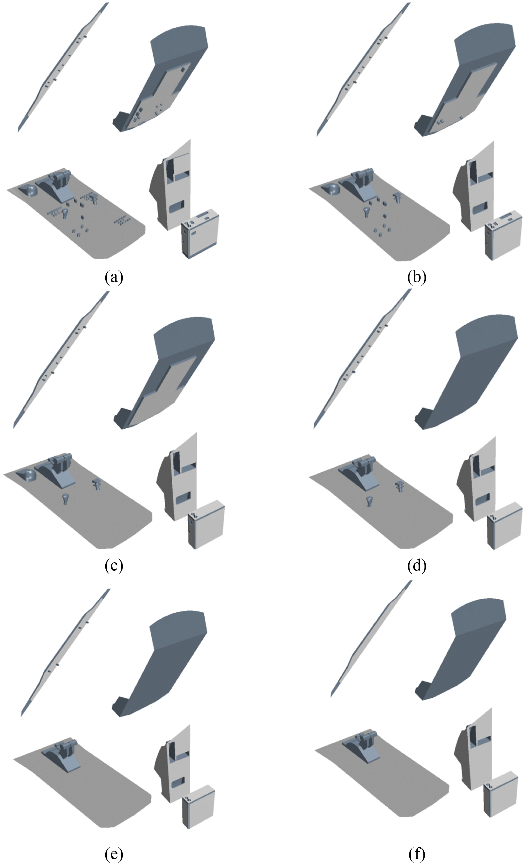
Figure 9: Some simplified parts of different versions (a) V1, (b) V2, (c) V3, (d) V4, (e) V5, (f) V6
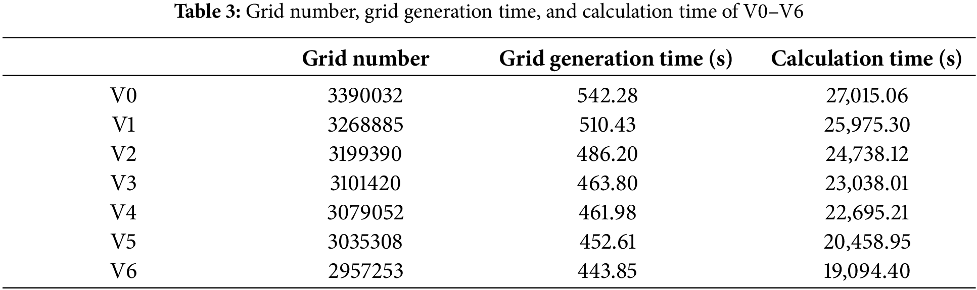
The above six simplified cases, V1 to V6, and the original version V0 are computed five times on the same 8-core computer. The average data of the grid number, grid generation time, and calculation time are obtained (as shown in Table 3). Compared to V0, V6 reduces the number of grid cells by 12.8%, grid generation time by 18.2%, and calculation time by 29.3%, indicating a significant improvement in computational efficiency.
Several points in front of the pilots’ and observers’ chests are selected, which are shown in Fig. 10, comparing the temperature and velocity on these points. The temperature and velocity deviation caused by different degrees of simplification are shown in Fig. 11. When the suppression degree reaches 14%, the absolute temperature deviation is 0.18°C, with a relative temperature deviation of 0.75%. The absolute velocity deviation is 0.016 m/s, with a relative velocity deviation is 21.82%.
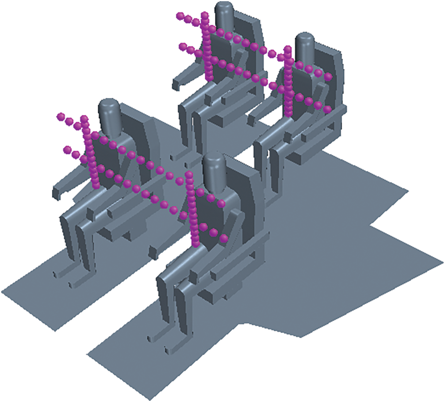
Figure 10: Points selected for comparing simulation results in six simplified versions
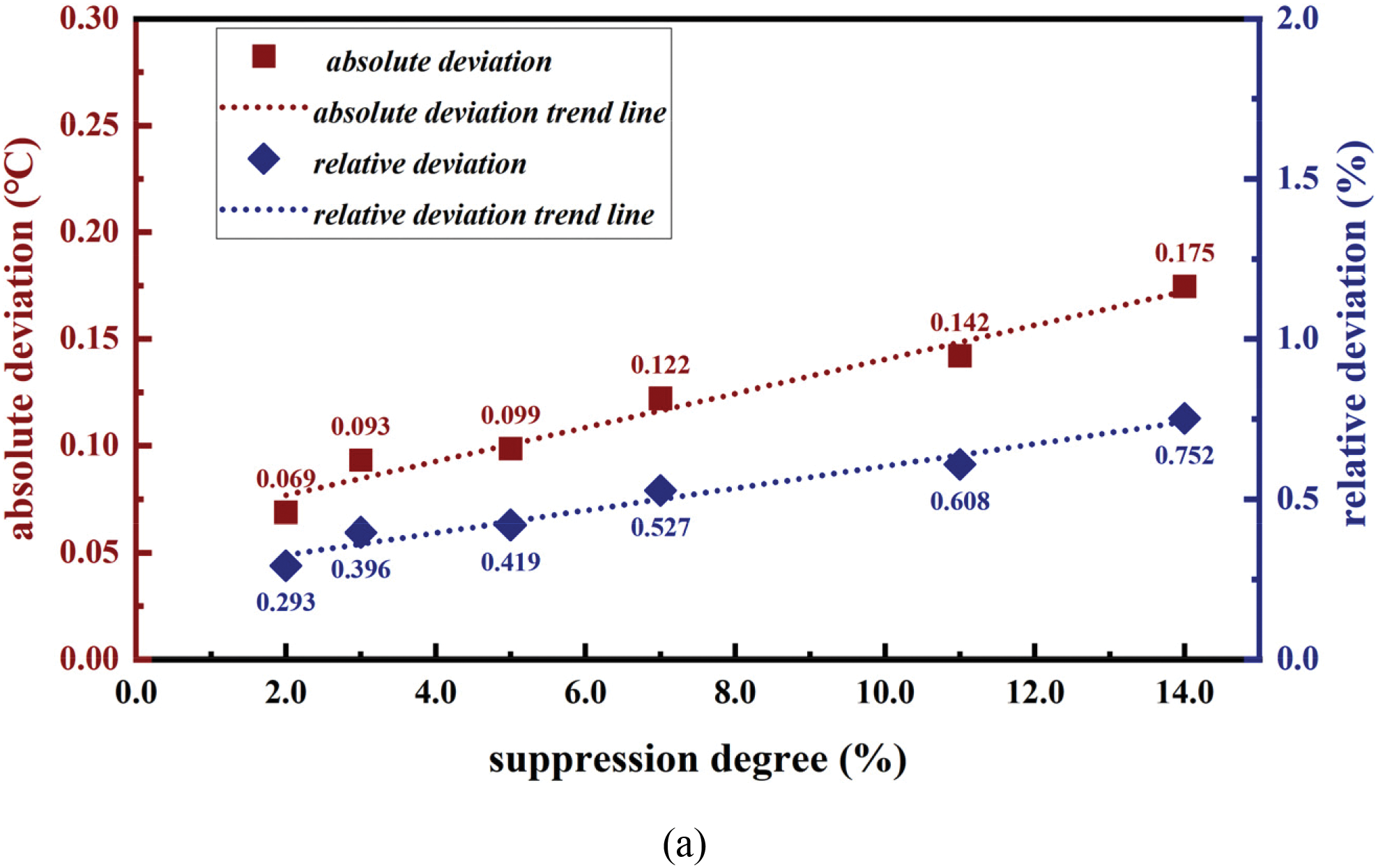
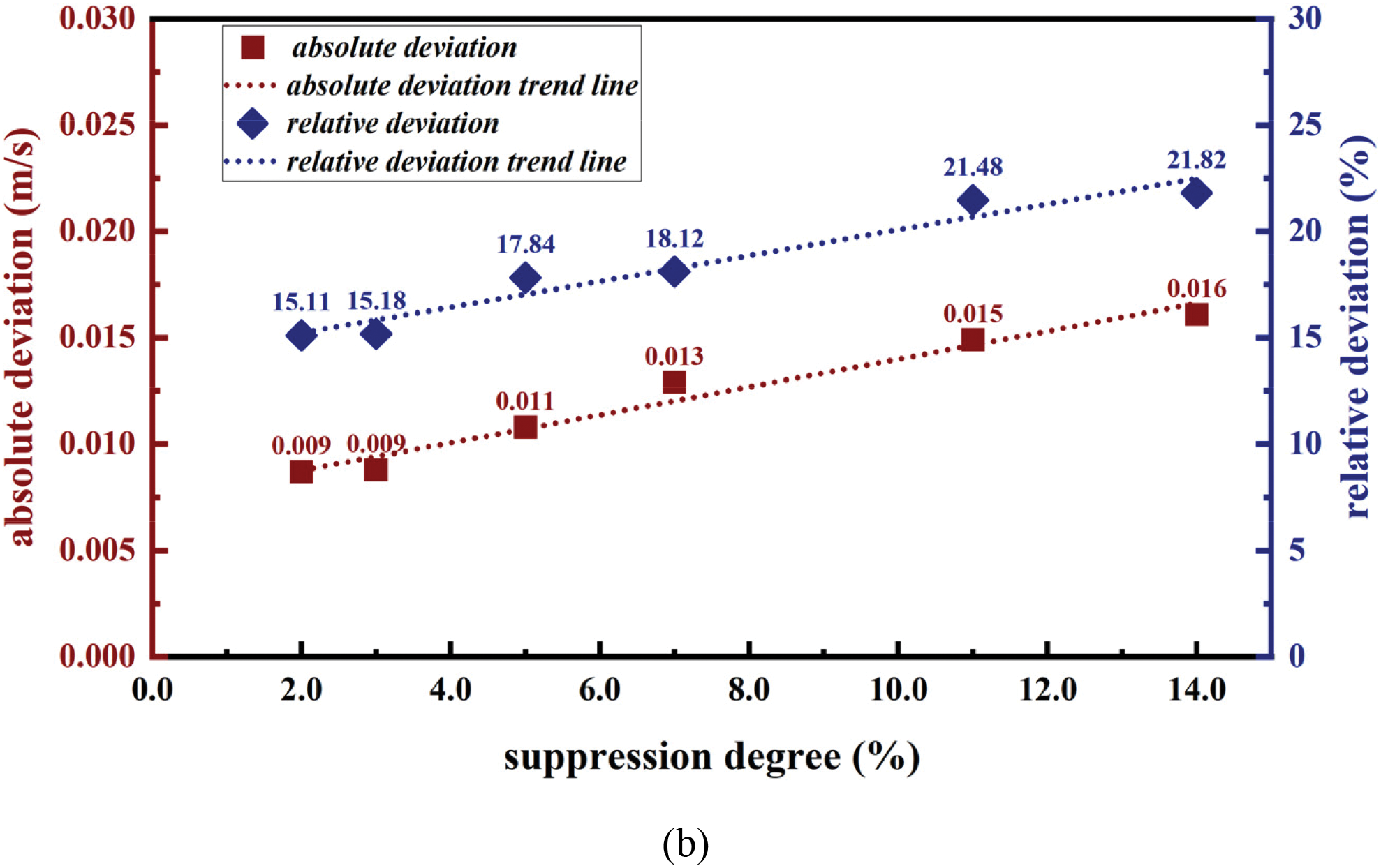
Figure 11: Deviation caused by different suppression degrees of (a) temperature; (b) velocity
According to the results of SAM, detailed features with different GSL should have different simplification deviations under the same suppression degree. Therefore, the detailed features with different GSL values are studied separately. The simplification versions are shown in Table 4. Still selecting the coordinate points in Fig. 10, the temperature deviation caused by simplification is shown in Fig. 12, and the velocity deviation is shown in Fig. 13.
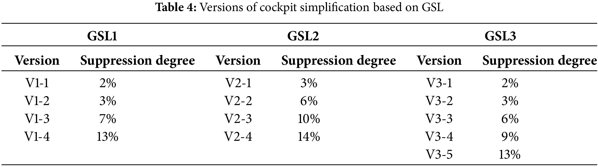
Figure 12: Temperature deviation caused by different suppression degrees of GSL1, GSL2, and GSL3: (a) absolute deviation, (b) relative deviation
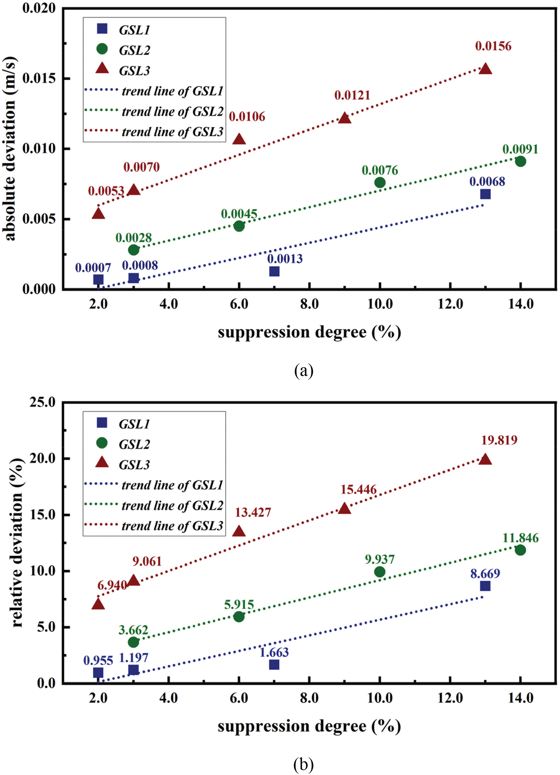
Figure 13: Velocity deviation caused by different suppression degrees of GSL1, GSL2, and GSL3: (a) absolute deviation, (b) relative deviation
4.3 Simplification Standards Determination through ESM
Calculate the deviations of the temperature field and the velocity field for all the simplified versions according to Eqs. (17) and (18) and plot the data points in Figs. 12 and 13 based on different GSL categories.
It can be seen that the calculation deviation and suppression degree show a linear growth relationship for the surfaces of each GSL. At the same suppression degree, the higher the GSL of the simplified surface, the greater the calculation deviation. The deviation caused by simplifying the surface of GSL3 is approximately 3–5 times that of simplifying the surface of GSL1. Additionally, the higher the GSL of the surface, the greater the slope of the deviation growth trend line. Increasing the same degree of suppression will result in a greater calculation deviation increase for surfaces with higher GSL. The relative temperature and velocity deviation caused by suppressing all detailed features with DCS less than 14% is 0.75% and 21.82% (not considering GSL), which is similar to the deviation results of only simplifying GSL3 detailed features to the same extent. This indicates that the calculation deviation of the DSM is mainly caused by the simplification of GSL3 detailed features. Thus, the suppression degree should be reduced for high GSL detailed features and be increased for low GSL detailed features to reduce calculation deviation.
The suppression degree should be determined by the acceptable physical field deviation. Based on the maximum acceptable physical field deviation and the fitted trend lines, the maximum suppression degree of detailed features with different GSLs can be obtained and used as the standards for simplification. Therefore, the simplification standards for the cockpit have been determined: to ensure that the temperature relative deviation after simplification is less than 0.2% and the velocity relative deviation is less than 8%, the suppression degree of detailed features with GSL1 should be less than 15%, detailed features with GSL2 should be less than 10%, and detailed features with GSL3 should be less than 3%. This standard can provide guidance for the simplification of cockpit models, facilitating the improvement of grid generation and computational efficiency in further simulation studies.
A geometric model simplification strategy has been developed in this study, comprising three components: Sensitivity Analysis Method (SAM), Detail Suppression Method (DSM), and Evaluation Standards Method (ESM). This article successfully simplified a cockpit model by applying this strategy, validating the effectiveness of the strategy, and addressing three issues: where to simplify, how to simplify, and to what extent. The simplification standard for the studied cockpit was obtained: to ensure that the temperature relative deviation after simplification is less than 0.2% and the velocity relative deviation is less than 8%, the suppression degree should not exceed 15% for details with GSL1, 10% for details with GSL2, and 3% for details with GSL3.
However, the limitation must be acknowledged in the research of this paper. The proposed geometric model simplification strategy has merely been successfully applied to the cockpit model employed in this paper, and its general applicability remains unproven. In future work, more investigations can be conducted for different geometric models, such as cockpits of other types, ship cabins, and automobile cabins. Moreover, the strategy can even be classified and optimized under different types of geometric models to accommodate their specific characteristics.
Acknowledgment: The authors thank anonymous reviewers and journal editors for their valuable comments, which significantly improved this paper.
Funding Statement: The research presented in this paper was supported by the National Natural Science Foundation of China (Grant No. 51878442).
Author Contributions: The authors confirm contribution to the paper as follows: study conception and design: Meng Zhao, Jiaao Liu; data collection: Meng Zhao, Jiaao Liu; analysis and interpretation of results: Meng Zhao, Jiaao Liu, Yudi Liu, Zhengwei Long; draft manuscript preparation: Meng Zhao, Jiaao Liu. All authors reviewed the results and approved the final version of the manuscript.
Availability of Data and Materials: The data supporting this article are available upon request.
Ethics Approval: Not applicable.
Conflicts of Interest: The authors declare no conflicts of interest to report regarding the present study.
References
1. Qiao G, Zhang T, Barakos GN. Numerical simulation of distributed propulsion systems using CFD. Aerosp Sci Technol. 2024;147(2024):109011. doi:10.1016/j.ast.2024.109011. [Google Scholar] [CrossRef]
2. Butler C, Newport D, Geron M. Optimising the locations of thermally sensitive equipment in an aircraft crown compartment. Aerosp Sci Technol. 2013;28(2013):391–400. doi:10.1016/j.ast.2012.12.005. [Google Scholar] [CrossRef]
3. Zhang Y, Liu J, Pei J, Li J, Wang C. Performance evaluation of different air distribution systems in an aircraft cabin mockup. Aerosp Sci Technol. 2017;70(4):359–66. doi:10.1016/j.ast.2017.08.009. [Google Scholar] [CrossRef]
4. Zhou Q, Ooka R. Comparison of different deep neural network architectures for isothermal indoor airflow prediction. Build Simul. 2020;13(6):1409–23. doi:10.1007/s12273-020-0664-8. [Google Scholar] [CrossRef]
5. Zhao Y, Liu Z, Li X, Zhao M, Liu Y. A modified turbulence model for simulating airflow aircraft cabin environment with mixed convection. Build Simul. 2020;13(3):665–75. doi:10.1007/s12273-020-0609-2. [Google Scholar] [PubMed] [CrossRef]
6. Duan R, Liu W, Xu L, Huang Y, Shen X, Lin C, et al. Mesh type and number for CFD simulations of air distribution in an aircraft cabin. Numer Heat Transf Part B: Fund. 2015;67(6):489–506. doi:10.1080/10407790.2014.985991. [Google Scholar] [CrossRef]
7. Ntinas GK, Shen X, Wang Y, Zhang G. Evaluation of CFD turbulence models for simulating external airflow around varied building roof with wind tunnel experiment. Build Simul. 2018;11(1):115–23. doi:10.1007/s12273-017-0369-9. [Google Scholar] [CrossRef]
8. Broderick CR, Chen Q. A simple interface to computational fluid dynamics programs for building environment simulations. Indoor Built Environ. 2000;9(6):317–24. doi:10.1177/1420326X0000900603. [Google Scholar] [CrossRef]
9. Ahmadi J, Mahdavinejad M, Larsen OK, Zhang C, Zarkesh A, Asadi S. Evaluating the different boundary conditions to simulate airflow and heat transfer in Double-Skin Facade. Build Simul. 2022;15(5):799–815. doi:10.1007/s12273-021-0824-5. [Google Scholar] [CrossRef]
10. Shimada K. Current Issues and trends in meshing and geometric processing for computational engineering analyses. J Comput Inf Sci Eng. 2011;11(2):021008. doi:10.1115/1.3593414. [Google Scholar] [CrossRef]
11. Lee S. 19.A CAD-CAE integration approach using feature-based multi-resolution and multi-abstraction modeling techniques. Comput-Aided Des. 2015;37(9):941–55. doi:10.1016/j.cad.2004.09.021. [Google Scholar] [CrossRef]
12. Su X, Guo Y, Long Z, Cao Y. Numerical study of the influence of the atmospheric pressure on the thermal environment in the passenger cabin. Build Simul. 2023;17(2):253–65. doi:10.1007/s12273-023-1064-7. [Google Scholar] [CrossRef]
13. White D, Saigal S, Owen S. Meshing complexity: predicting meshing difficulty for single part CAD models. Eng Comput. 2005;21(1):76–90. doi:10.1007/s00366-005-0002-x. [Google Scholar] [CrossRef]
14. Danglade F, Véron P, Pernot J, Fine L. Estimation of CAD model simplification impact on CFD analysis using machine learning techniques. Comput-Aided Des Appl (CAD 2015). 2015;53–57. [Google Scholar]
15. Zienkiewicz OC, Taylor RL. The Finite element method. London: McGraw-Hill; 1994. vol. 3. [Google Scholar]
16. Thakur A, Banerjee AG, Gupta SK. A survey of CAD model simplification techniques for physics-based simulation applications. Comput-Aided Des. 2009;41(2):65–80. doi:10.1016/j.cad.2008.11.009. [Google Scholar] [CrossRef]
17. Li M, Nan L. Feature-preserving 3D mesh simplification for urban buildings. ISPRS J Photogramm Remote Sens. 2021;173(1):135–50. doi:10.1016/j.isprsjprs.2021.01.006. [Google Scholar] [CrossRef]
18. Xu C, Xie Y, Huang S, Zhou S, Zhang W, Song Y, et al. A coupled analysis on human thermal comfort and the indoor non-uniform thermal environment through human exergy and CFD model. J Build Eng. 2023;74(2023):106845. doi:10.1016/j.jobe.2023.106845. [Google Scholar] [CrossRef]
19. Shen X, Cao Z, Liu H, Cong B, Zhou F, Ma Y, et al. Inverse tracing of fire source in a single room based on CFD simulation and deep learning. J Build Eng. 2023;76:107069. doi:10.1016/j.jobe.2023.107069. [Google Scholar] [CrossRef]
20. Sun H, An L, Feng Z, Long Z. CFD simulation and thermal comfort analysis in an airliner cockpit. J Tianjin Univ (Sci Technol). 2014;47(4):298–303 (In Chinese). [Google Scholar]
21. Yan Y, Li X, Tao Y, Fang X, Yan P, Tu J. Numerical investigation of pilots’ micro-environment in an airliner cockpit. Build Environ. 2022;217:109043. doi:10.1016/j.buildenv.2022.109043. [Google Scholar] [CrossRef]
22. Lei L, Zheng H, Xve Y, Liu W. Inverse modeling of thermal boundary conditions in commercial aircrafts based on Green’s function and regularization method. Build Environ. 2022;217:109062. doi:10.1016/j.buildenv.2022.109062. [Google Scholar] [CrossRef]
23. Han Y, Zhang Y, Gao Y, Hu X, Guo Z. Vortex structure of longitudinal scale flow in a 28-row aircraft cabin. Build Environ. 2022;222:109362. doi:10.1016/j.buildenv.2022.109362. [Google Scholar] [CrossRef]
24. Hou Y, You R. Investigating the impact of gaspers on airborne disease transmission in an economy-class aircraft cabin with personalized displacement ventilation. Build Environ. 2023;245(1):110963. doi:10.1016/j.buildenv.2023.110963. [Google Scholar] [CrossRef]
25. Yin H, Shen X, Huang Y, Feng Z, Long Z, Duan R, et al. Modeling dynamic responses of aircraft environmental control systems by coupling with cabin thermal environment simulations. Build Simul. 2016;9(4):459–68. doi:10.1007/s12273-016-0278-3. [Google Scholar] [CrossRef]
26. Li X, Yan Y, Fang X, Fang X, He F, Tu J. Towards understanding of inhalation exposure of pilots in the control cabin environment. Build Environ. 2023;242:110572. doi:10.1016/j.buildenv.2023.110572. [Google Scholar] [CrossRef]
27. Li X, Fang X, Yan Y. In-depth investigation of air quality and CO2 lock-up phenomenon in pilots’ local environment. Exp Comput Multiph Flow. 2024;6(2):170–9. [Google Scholar]
28. Liu W, Duan R, Chen C, Lin C, Chen Q. Inverse design of the thermal environment in an airliner cabin by use of the CFD-based adjoint method. Energy Build. 2015;104:147–55. [Google Scholar]
29. Cao Q, Liu M, Li X, Lin C, Wei D, Ji S, et al. Influencing factors in the simulation of airflow and particle transportation in aircraft cabins by CFD. Build Environ. 2022;207:108413. [Google Scholar] [PubMed]
30. Wei Y, Zhang T, Jin H. Rapid prediction of airborne gaseous pollutant transport in aircraft cabins based on proper orthogonal decomposition and the Markov chain method. Build Environ. 2023;228:109816. [Google Scholar]
31. Yang X. Research on model simplification and validation method for auto side impact simulation [master thesis]. China: Chongqing University; 2018 (In Chinese). [Google Scholar]
32. Wang Q. Feature-based responses prediction method for simplified CAE models based on machine learning and its application in vehicle safety [master thesis]. China: Chongqing University; 2019 (In Chinese). [Google Scholar]
33. Kang L, Zhou X, Hooff T, Blocken B, Gu M. CFD simulation of snow transport over flat, uniformly rough, open terrain: impact of physical and computational parameters. J Wind Eng Ind Aerod. 2018;177:213–26. [Google Scholar]
34. Li S, Wang H, Liu X, Guo P, Wang X, Chu Y. Simulation of wind profile in coastal areas by using a structural wind-resistant moving vehicle tester: CFD and experimental investigations. J Build Eng. 2022;48:103951. [Google Scholar]
35. Li M. Review on engineering analysis reliable CAD model simplification. J Comput-Aided Des Comput Graph. 2015;27(8):1363–75 (In Chinese). [Google Scholar]
36. Gopalakrishnan SH, Suresh K. A formal theory for estimating defeaturing-induced engineering analysis errors. Comput-Aided Des. 2007;39(1):60–8. [Google Scholar]
37. Gopalakrishnan SH, Suresh K. Feature sensitivity: a generalization of topological sensitivity. Finite Elem Anal Des. 2008;44(11):696–704. [Google Scholar]
38. Turevsky I, Gopalakrishnan SH, Suresh K. Defeaturing: a posteriori error analysis via feature sensitivity. Int J Numer Methods Eng. 2008;76(9):1379–401. [Google Scholar]
39. Turevsky I, Gopalakrishnan SH, Suresh K. An efficient numerical method for computing the topological sensitivity of arbitrary-shaped features in plate bending. Int J Numer Methods Eng. 2009;79(13):1683–702. doi:10.1002/nme.2637. [Google Scholar] [CrossRef]
40. Taroco E, Buscaglia G, Feljóo R. Second-order shape sensitivity analysis for nonlinear problems. Struct Multidiscipl Optim. 1998;15(2):101–13. doi:10.1007/BF01278496. [Google Scholar] [CrossRef]
41. Antolín P, Chanon O. Analysis-aware defeaturing of complex geometries with Neumann features. Int J Numer Methods Eng. 2023;125(3):e7380. doi:10.1002/nme.7380. [Google Scholar] [CrossRef]
42. Huang H, Ekici K. A discrete adjoint harmonic balance method for turbomachinery shape optimization. Aerosp Sci Technol. 2014;39:481–90. doi:10.1016/j.ast.2014.05.015. [Google Scholar] [CrossRef]
43. Liu M, Matsubara K, Hasegawa Y. Adjoint-based shape optimization for radiative transfer in porous structure for volumetric solar receiver. Appl Therm Eng. 2024;246(1):122899. doi:10.1016/j.applthermaleng.2024.122899. [Google Scholar] [CrossRef]
44. Tang X, Luo J, Liu F. Aerodynamic shape optimization of a transonic fan by an adjoint-response surface method. Aerosp Sci Technol. 2017;68(2):26–36. doi:10.1016/j.ast.2017.05.005. [Google Scholar] [CrossRef]
45. Altaf Z, Babar MI, Salamat S. Multi-objective shape optimization of doubly offset serpentine diffuser using Adjoint method. Int J Heat Fluid Flow. 2023;102(9):109157. doi:10.1016/j.ijheatfluidflow.2023.109157. [Google Scholar] [CrossRef]
46. Liu F, Chen H, Yuan H, Zhang T, Liu W. Shape optimization of the exhaust hood in machining workshops by a discrete adjoint method. Build Environ. 2023;244:110764. doi:10.1016/j.buildenv.2023.110764. [Google Scholar] [CrossRef]
47. Sun R, Gao S, Zhao W. An approach to B-rep model simplification based on region suppression. Comput Graph. 2010;34(5):556–64. doi:10.1016/j.cag.2010.06.007. [Google Scholar] [CrossRef]
48. Cao W. Survey of automated geometry model simplification for CAE analysis. J Comput-Aided Des Comput Graph. 2017;29(3):406–18 (In Chinese). [Google Scholar]
49. Wang Y, Lin Y, Eri Q, Kong B. Flow and thrust characteristics of an expansion-deflection dual-bell nozzle. Aerosp Sci Technol. 2022;123(5):107464. doi:10.1016/j.ast.2022.107464. [Google Scholar] [CrossRef]
50. Yu T, Wu X, Yu Y, Li R, Zhang H. Establishment and validation of a relationship model between nozzle experiments and CFD results based on convolutional neural network. Aerosp Sci Technol. 2023;142:108694. doi:10.1016/j.ast.2023.108694. [Google Scholar] [CrossRef]
51. Sun P, Zhou L, Wang Z, Shi J. Influences of geometric parameters on serpentine nozzles for turbofan. Aerosp Sci Technol. 2023;136(10):108224. doi:10.1016/j.ast.2023.108224. [Google Scholar] [CrossRef]
52. Zhang M, Fan F, Hu X. A comparative study on turbulence models for indoor air flow field. Energy Eng, 2018(2):52–9 (In Chinese). [Google Scholar]
53. He W. Experiment and simulation of sensible heat loss for occupant in aircraft cabin [master thesis]. China: Tianjin University; 2014 (In Chinese). [Google Scholar]
54. Song S, Guo X. Boussinesq approximation and numerical simulation of natural convection in a closed square cavity. Chin Q Mech. 2012;33(1):60–7 (In Chinese). [Google Scholar]
55. Li X, Yan Y, Fang X, Tu J. Numerical studies of indoor particulate and gaseous micropollutant transport and its impact on human health in densely-occupied spaces. Environ Pollut. 2024;342:123031. doi:10.1016/j.envpol.2023.123031. [Google Scholar] [CrossRef]
56. Ferziger JH, Perić M, Street RL. Computational methods for fluid dynamics: basic concepts of fluid flow. 4th ed. Cham: Springer; 2020. [Google Scholar]
Cite This Article
 Copyright © 2025 The Author(s). Published by Tech Science Press.
This work is licensed under a Creative Commons Attribution 4.0 International License , which permits unrestricted use, distribution, and reproduction in any medium, provided the original work is properly cited.
 Downloads
 Citation Tools