Stability Prediction in Smart Grid Using PSO Optimized XGBoost Algorithm with Dynamic Inertia Weight Updation

1  Introduction

SG (Smart Grid) is comprised of control stations, communication lines, distributors, and transformers, which aim to supply power from electrical plant sources to consumers. Power generated in electric grids is millions of megawatts through which power is distributed across numerous demographic areas [1]. Hence, efficient power supply management [2] to different consuming domains like smart cities, industries, and organizations is essentially important. To maintain stability in the smart grid system, power generated needs to match the required demand and maintain storage for immediate level outages. Moreover, it is necessary to afford adequate capability for stabilizing voltage at each portion. Stability is generally measured in terms of frequency [3]. When energy generated is greater than the rate of consumption, then there occurs an increase in frequency. It gradually decreases when consumption is greater than the generated. Therefore, to maintain grid stability, it is significant to take continuous actions on the level of consumption and generation. Technologies have been developed in all sectors regarding administration and production [4].

Similarly, automatic controlling and monitoring of power-grid structures have also been designed. However, meeting certain requirements like stability, resiliency, and reliability has been challenging due to dynamic variations in grid topology and power utilities [5]. Managing demands in electric grids without changing grid structure is assumed to be a challenging task for smart grids in struggling to provide generators for fluctuating consumption and production [6]. For providing demand-level grid management, the capability of maintaining stability in a grid concerning modifications in prices and varying levels of price sensitivity along with reaction times due to changes in prices exhibited by consumers and producers is considered essential in yielding expected stability outcomes [7].

Smart grids are generally deployed with intelligent systems for catering to the changing requirements in power supply [8]. Integration of AI-based algorithms in the grid has assisted in monitoring the power flow and fluctuations [9]. ML (Machine Learning) model with power-dissipation units has been used for predicting stability. To distribute power effectively to control stations, the stability of SG is important, which has been accomplished through MLSTM (Multi-directional Long Short-Term Memory) and has been experimented on the SG dataset from the UCI Machine Learning Repository. Stability has been predicted by considering the attribute information concerning the power consumed and produced level, coefficients regarding price elasticity, and electricity-producer values. The application of a fuzzy-based approach in the suggested research [10] has characterized an optimized level of accuracy in decentralized SG systems. It has focused on the influence of specific input attributes over SG stability. It also has analyzed the effects of overlapping certain attributes over other attributes from the perspective of stability. Balance ineffective consumption and generation has been considered a significant factor in smoothening power-grid supply [11]. Mismatching between demand and supply considerably increases the cost for customers and service providers and sometimes has crippled the complete grid. Focusing on stability, recommended research [12] has provided a real-time and incentive-oriented demand-response technique for SG with the utilization of reinforcement learning along with a neural network which has enhanced reliability with effective balancing on energy with appropriate resource purchasing strategies in the grid [13,14]. Particularly, uncertainties have been handled in predicting the varying prices and demands for energy [15]. An optimal rate of incentives from different consumers has been obtained with the reinforcement-learning method, which has considered the benefits of both consumers and providers. Simulation outcomes have revealed that the considered incentive method-based algorithm has induced demand level participation and has promoted reliability by efficiently balancing energy resources. In addition to that, another real-time structure involved with the order reduction mechanism [16] has also provided stability with the utilization of the orthogonal decomposition technique. Snapshot matrix in sliding and sampling window has been used to extract significant system components through random singular-valued decomposition. After order reduction in the system, the linear framework has been estimated for the matrix [17]. Subsequently, the system’s state has been predicted with the sliding prediction. Accordingly, the stability index has been measured, which can forecast future stability in the prediction window. It also has estimated the limit of stability and predicted transient stability. Instability detection in first-swing and multi-swing has been performed, and stability of the system has been predicted through simulations with minimum computational complexities [18].

Even though conventional studies have provided many methodologies and techniques for the prediction analysis of energy consumption in smart cities to provide the energy source based on the demand minimum error rate in the prediction using regression, it still requires improvement in the accurate prediction of stability in smart grids. Moreover, the consumed energy prediction alone has not assisted in minimizing the unstable conditions but also required a regression model in preventing backdrops in SG [19]. Accurate measurement of power distribution and surge occurrence reduces the backdrops considerably. Hence, some of the common limitations for the validation of prediction have been analyzed from the existing literature and are listed as follows:

•   The stability prediction mechanism has extracted adequate information but can provide a better learning process in prediction by utilizing the prior data with reduced computational complexities [10].

•   The regression process can be enriched with larger datasets that provide effective outcomes instability by adding weighting factors that improve optimization in SG [12].

To this purpose, the ML-based regression method in stability prediction with effective pre-processing of input data is proposed in the present study for future predictions on SG stability. It incorporates and performs analysis on various attributes such as electricity prices and response-level characteristics of a participant in the calculation of the stability of the grid under various conditions. Variables such as electricity volume produced or consumed by every participant in the grid (P), reaction times (tau), and cost sensitivity (G) in fluctuating grid conditions. It is designed to predict grid stability from the sensitivity levels of variables. Moreover, the proposed research addresses the challenges of existing studies in attaining effective predictions on energy stability with smart city systems.

Based on the analysis made from various approaches, the aim and objective of the present research are framed as follows:

•   To predict stability for the smart city with the input data collected from the smart grid stability prediction dataset and perform pre-processing.

•   To perform regression with the modified Particle Swarm Optimization (PSO) Optimized XGBoost Algorithm with dynamic inertia weight adjustment to predict stability with minimized regression loss.

•   To evaluate the system with performance metrics such as MSE (Mean Square Error), RMSE (Root Mean Square Error and MAE (Mean Absolute Error) and to compare with existing algorithms for validating the efficacy of the model.

The paper is organized as follows. Section 2 shows the review of several existing studies related to stability estimation in the smart city based on SG systems. Section 3 outlines the proposed energy analysis with the regression algorithm utilized in the study. Section 4 provides performance analysis and internal comparative assessment with other algorithms. Finally, the proposed work is concluded in Section 5.

2  Literature Review

The following section discusses various techniques and methodologies utilized in the identification of stability maintained in smart city systems. In SG structure, disruptions in the normal delivery of power lead to instability in grid systems [20]. Numerous methodologies have been utilized for the determination of grid stability. Estimating the maximum power availability in the grid has utilized the demand-response structure, which determined the maximum degree of power balanced in smart cities in considered research [21]. Moreover, it has used parameters in determining the compensation effect of reactive power which balanced the maximum power. Aggregation of load measurements has provided a poor estimate level of parameters. Accuracy has affected the estimation of maximum power [22]. Individual load measurements have been undertaken in smart meters to provide improved estimates of parameters. The stability index measure has been utilized for estimating the instability complication. Bidirectional communication flow processed with the smart grid in the recommended methodology [23] has followed the concept of demand and supply. Stability prediction has been observed to be essential in enhancing consistency and reliability. Missing input values have been handled effectively, and the forecasting framework has utilized NN (Neural Network) in stability prognosis [24]. The model has been trained using the transfer functions such as purelin and tansig in hidden layers. The system’s performance has been evaluated using the 4-node network and exhibited better prediction performance when measured with respect to mean square error [25].

Assessment of the electrical flow in SG has been monitored by deploying the extreme-learning model in which learning-oriented optimization has been performed. Simulated-annealing methods have been utilized in the suggested research [26]. Stability in electric grid has been analyzed through the rising supply and demand requirements for smart cities. The essential need for IoT (Internet of Things) in energy generation has been investigated in [27]. Prediction algorithms such as naïve Bayes, support vector machine, logistic regression, decision tree, and optimized ANN (Artificial Neural Network) have been applied to smart energy grid-based datasets for predicting stability. Various metrics have been used in analyzing the stability performance [28]. Feature scaling methods and data-augmentation techniques applied to datasets have achieved better outcomes. Dynamic characteristics of SG need to be analyzed, and behavioral information of the grid provides effective reliability and management operation [29]. Particularly in the recommended study [30], the damping of electromechanical oscillations in an interconnected grid has been evaluated through a decision tree to classify inter-area-based oscillations [31]. For every generation of buses, a separate decision tree has been assigned to calculate oscillations. Since DT (Decision Tree) has the capability to lower computational complexity, it has been embedded into the phasor assessment with minimum cost [32]. Outcomes have evaluated contingency situations, and expected accuracy has been attained concerning stability. Disturbances and complications within the SG have been examined through robust DT, even during the loss of data from generators.

Electric grid stability is influenced by real-time electricity prices, along with reaction times and cost sensitivity in power users and producers [33]. Recommended research [34] has predicted changes in the frequency of the grid over a different period in a decentralized system and has provided control on the demand side of the grid. Electricity consumption and production have been administered to analyze the stability [35]. It has considered measurements on different variables of G, P, Tauquantifies, and Stbin concerning the pricing and mechanical influences. Accuracy degree and correlation of independent variables and input variables. It has highlighted feature selection significance in recognition of stability in the grid [36]. The SG has implemented demand-response without major changes in infrastructural requirements. Stabilization in considered methodology [37] has autonomously regulated the frequency based on the power demand.

SG is required to be stable to balance both demand and supply dynamically and economically through effective grid operation. Factors affecting the stability of the grid have been analyzed. Renewable energy sources are unpredictable on changing time scales [38]. Based on the volatile nature of the grid, fluctuations have occurred frequently, which is closely associated with the electricity rate. Simulation has been accomplished with the ML-based repository in which data normalization has been adopted to reduce the biased nature among various attributes [39]. The imbalance in data has been handled through data re-sampling methodologies. The suggested method has combined XGBoost with a random sampling technique, effectively predicting the fluctuations in frequency acquired from power grids. A better distribution and electricity management level in SG has contributed to the efficient future prediction of stability factors. In considering the infrastructure of SG, stability is an important metric in determining the efficiency of SG. Since fluctuations in flow and changes in parameter can cause mispredictions and incorrect decisions lead to dreadful consequences. Model-driven techniques with the ML-based methodology have been applied to SG management on stability [40]. Meta-model has aimed at mapping features from extracting data and importing obtained information in Neo4j has created graphs, and the DL (Deep Learning) model provided relevant target and input attributes has generated output through training. Prediction on future stability status has been explored through the previously collected information.

3  Proposed Methodology

The proposed method employs a stability prediction scheme in smart grids for analyzing the changes in energy utilities and to manage the power demand and supply efficiently in smart cities. The continuous monitoring and prediction of the energy consumed, and other significant assessment variables assist in the effective management and continuous power dispatch to different entities in SG. Existing research has suffered from limited stability performance with the experimentation on the SG stability-prediction dataset. Hence, the proposed system intends to enhance the efficiency of SG through the regression technique with the enhancements accomplished in the PSO algorithm to achieve an efficient future estimation of stability. The proposed algorithm keeps SG intact even after fluctuations and other disturbances. The architecture diagram of the proposed model is illustrated in Fig. 1.

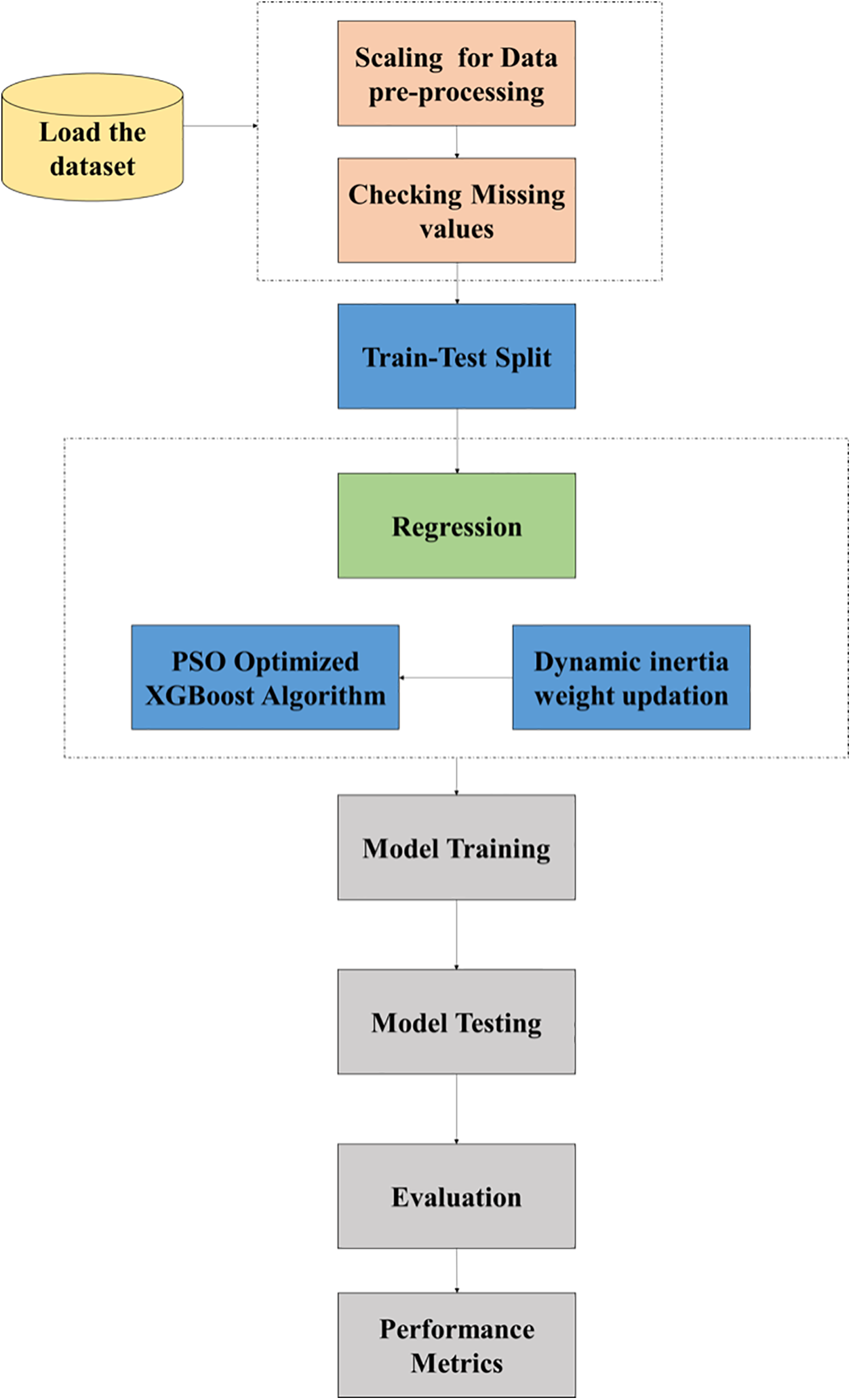
Figure 1: Overall architecture for proposed prediction system

The proposed regression framework and the entire working process of the model are given in Fig. 1, in which the process is segregated into two stages, pre-processing, and regression. The input dataset taken for the proposed analysis is the Smart-Grid Stability Prediction dataset. The data in the dataset are taken from the residential areas concerning the information about the energy consumed based on various utilities. The fluctuations and changing demand for electricity are recorded on a timely basis hourly, daily, and weekly. The observations are performed based on data collected from the dataset which assists in meeting the demand for energy in SG at all times.

Moreover, it regains the system to normal operating conditions and maintains stability in the power flow within the network. The collected data are then pre-processed by feature scaling which is performed for standardization of an independent set of features occurring in data to a fixed range. It is accomplished during the pre-processing stage for handling higher variance in the magnitude of values. Followed by that, it checks for missing values since un-treated values create complications in real-time datasets and produce biased outcomes. After that, the pre-processed data are split into 80% training and 20% testing of the model, which then passes on to the regression framework. Finally, effective prediction is being performed with the modified PSO Optimized XGBoost algorithm updated with dynamic inertia weight for efficient future prediction on stability. The main intention of integrating PSO with XGBoost is mainly performed for improving the prediction accuracy through optimization with significant parameters of XGBoost through PSO. Moreover, PSO’s dynamic weight update factor improves the optimization outcome since it changes linearly based on PSO performance through which local and global optimum solutions are attained. The outcome of the proposed model can achieve future predictions on stability in SG efficiently. The structure of the SG system incorporated with the proposed algorithm is depicted in Fig. 2.

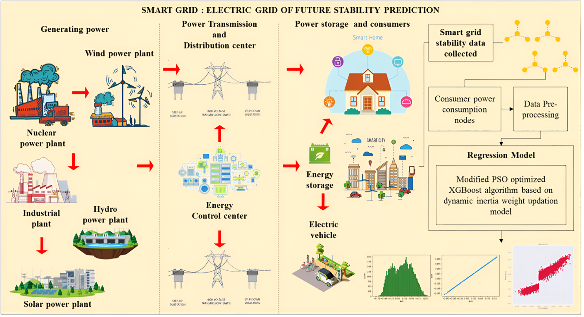
Figure 2: Smart grid for future stability prediction

The entire framework of the proposed SG model is given in Fig. 2, and the process flow is depicted. Initially, energy is generated from different sources like nuclear plants, industrial plants, hydro, solar, and wind power plants. Then, power is transmitted through transmission lines and distributed to the energy control center. Next, the generated energy is stored in the power storage area. Finally, energy is distributed to smart cities, electric vehicles, and other entities from the storage hub. From the smart-city distribution pattern, SG stability data is being collected and forms a consumer power consumption node structure with a four-node topology. Collected data are pre-processed, and the proposed regression model is applied for predictions. Regression is achieved through PSO Optimized XGBoost algorithm with dynamic inertia weight adjustment framework and predicts the energy stability in SG. The present regression system is validated through metrics MSE (Mean Square Error), MAE (Mean Absolute Error), and RMSE (Root Mean Squared Error). It can provide a lower error in the difference between the predicted value and the actual value.

3.1 Regression Using Modified PSO Optimized XGBoost with Dynamic Inertia Weight Updation

The proposed work uses the regression model to predict stability based on continuous outcome patterns of energy. The process is accomplished by adopting PSO, in which XGBoost parameters are tuned for better performance. In addition, dynamic inertia weight is updated, drawing preliminary information together to make an accurate prediction. The proposed regression flow operation is illustrated in the given Fig. 3.

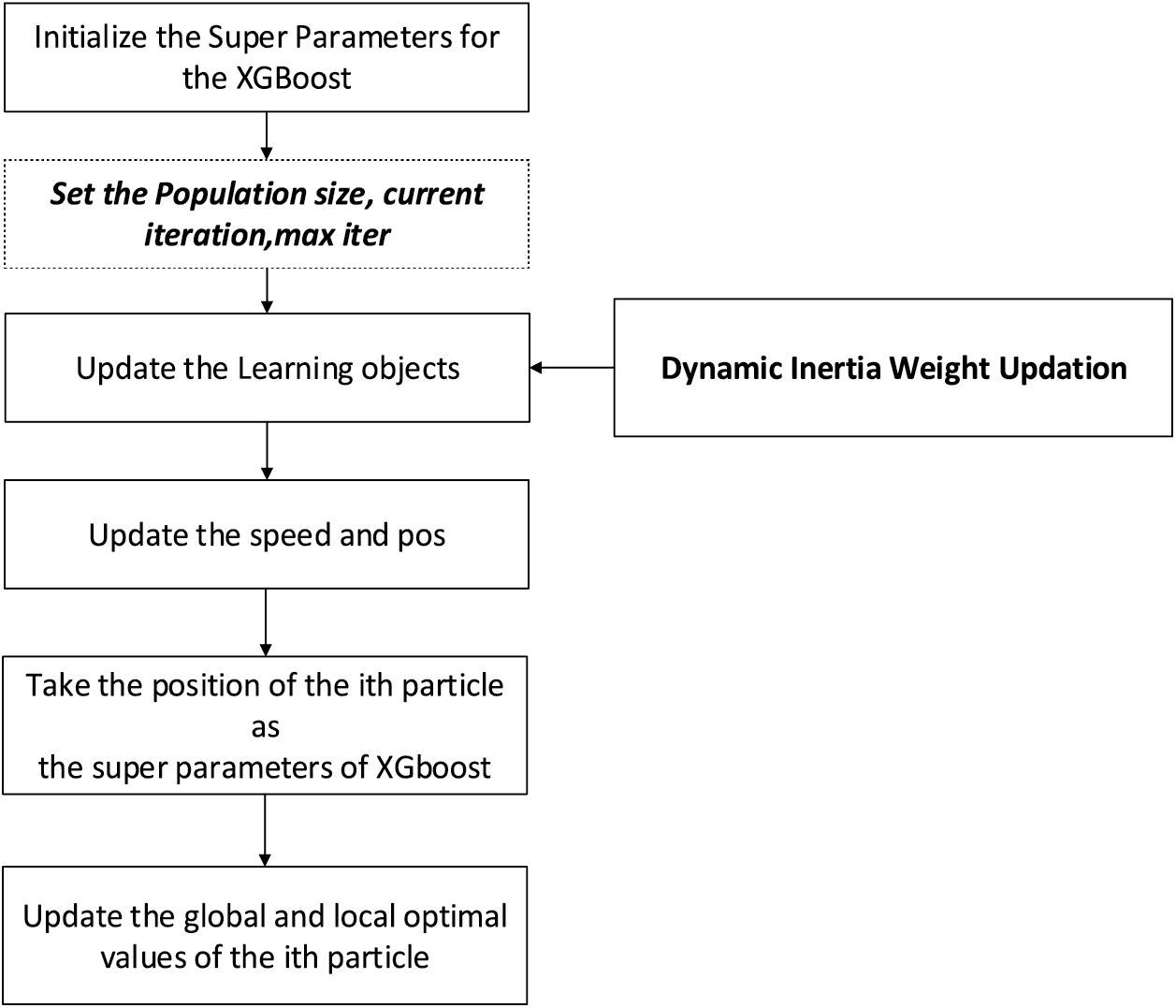
Figure 3: Workflow of proposed algorithm

From Fig. 3, it is clear that the hyperparameters for XG-Boost are initialized with the determination of the population size of particles. Particles search for the best solution in the search area. While learning objects are updated with the dynamic inertia weight, the speed and position vectors are updated in the PSO algorithm. It helps in the determination of the path and position of particles. Followed by that, the position of an ith particle in search space is chosen as the super-parameters of XGBoost, which updates the local and global optimum values for the ith particle. The computational method optimizes the problem by iteratively improving the solution. Population-oriented regression is the robust technique for obtaining the best solution. Enhancements involved in the algorithm are discussed as follows.

3.1.1 PSO Algorithm

PSO is an evolutionary technique utilized in searching for an optimal solution to a problem. PSO is relatively simple to implement and requires fewer parameters to adjust compared to other optimization algorithms, which can simplify the modeling process. Its flexibility allows it to be applied to a wide range of optimization problems. Likewise, the PSO algorithm is inherently adaptable, allowing it to respond dynamically to changes in grid conditions. This adaptability makes it suitable for real-time applications where quick adjustments are necessary to maintain stability. Besides, PSO excels in global optimization, helping to avoid local minima. This is particularly beneficial in high-dimensional spaces, where other methods struggle. Moreover, integrating PSO with advanced techniques like XGBoost leverages the strengths of both methods, thus combining the optimization capabilities of PSO with the predictive power of XGBoost. Owing to these factors, PSO is opted by the proposed work over other algorithms.

1.    It generally operates by mimicking the nature of birds in exchanging information. In this algorithm, every solution is considered a bird in search space, referred to as a particle. Each particle is associated with fitness values evaluated with the fitness function and optimized with velocities that direct the position of flying particles. It is initialized with the population of random solutions and searches the optimal values with the update of generations. PSO has the advantage of adjusting minimum parameters and is easier to implement. In PSO, the population is called a swarm, and every individual is regarded as a particle. The ith particle with iteration h is involved with two attributes as follows.

2.    The present position in N-dimensional search-space of Aih=(a1h,…,adh,…,aDh) where a1kϵ[lwn,upn],1≤d≤D,lwdis lower and,upd upper bound in d dimension, respectively.

3.    Present velocity Bih=b1h,…,bdh,…,bDh which is being bounded with maximum level of velocity Bmaxh=(bmax,1h,…,bmax,dh,…,bmax,Dh) and with minimum velocity Bminh=(bmin,1h,…,bmin,dh,…,bmin,Dh).

Every particle is updated with the two best values in each search iteration. The initial value is the best solution that has been achieved, which is referred to as the pbest. The other best value, tracked through PSO, is considered the best value acquired by particles in the population. Therefore, it is being referred to as the global-best recognized as gbest. When particles participate as the population in the form of topological neighbors, the local-best value is signified as lbest. Every particle is updated with two best values for every search-level iteration. The initial best value is the fitness solution that has been achieved stored so far, and that value is referred to as pbest. The other best value being tracked by the PSO is the best value acquired by a particle in the population. Such the best solution is recognized as global-best (gbest). When particles participate in population with neighbors and attain, the best values signified as local-best (lbest). After the prediction of two values, the particle is updated with position and velocity using the below formulas:

Bi(h+1)=w(Bi(h)+lf1e1(PPi(h)−Ai(h)+lf2e2(BPg(h)−Ai(h)))(1)

Ai(h+1)=Ai(h)+Bi(h+1)(2)

PPi is recognized as the best previously obtained position of an ith particle named pbest. Two forms of PSO basoccur based on BPg being the best position within all particles in a swarm during the global version. If BPg is picked up from limited adjacent particles of population termed as local version. PPi and BPg are estimated in the following equation as

PPi=(PPi:of(Ai)≥of(PPi)Ai:of(Ai)<of(PPi))(3)

BPgϵ{PP0,PP1,…,PPm}|of(BPg)=min(of(PP0),of(PP1),…,of(PPm))(4)

Which variable is measured as an objective function in which tp ≤ TP and TP is the overall number of particles. From Eqs. (1) and (2), h indicates the number of iterations, and If1, and If2 are factors used in learning where If1 = If2 = 2, which has complete control over particles moving around a single iteration. Variables e1 and e2 are attributes from two similar random sequences in range (0,1):r1∼U(0,1);r2∼U(0,1). Attribute w is the representation of inertia weight in the range of [0,1]. A larger inertia weight provides global exploration value, and a smaller inertial weight delivers a local exploration area for fine-tuning search space. When the expected fitness-value BPg is reached or maximum-generations have been grasped, iterations are terminated.

3.1.2 Dynamic Inertia Weight Update with PSO

PSO techniques generally share the information of local-best and global-best solutions to the next-level generation of particles. The present research provides modified PSO, which utilizes dynamic inertia-weight represented as dim, which decreases based on an increase in iterative generation. The best solution BPg is obtained from the current population, which remembers previously obtained the best position for every individual PPi in the swarm. In the case of search space with dim as the dimensional vector for n as particles form a colony. The jth particle represents a dim-dimensional vector with Aj=(j=1,2,3,…,n). It refers that jth particle located at Aj=(a1,…,an,…,aDim)(j=1,2,…,n) in search-space. The position of every particle provides the potential outcome. The particle’s fitness is calculated by involving the particle fitness in the expected objective-function. Ai is found to be better when the fitness outcome is lower. Accordingly, ith particle velocity is also a dim dimensional vector represented by Bj=(bj1,bj2,…,bjDim). The best position of the ith particle as PPi=(ppi1,ppi2,…,ppjDim) and best position the colony as BPg=(bp1,bp2,…,bpjDim), respectively.

Bi(h+1)=DIW′⊙(Bj(h)+lf1e1(PPj(h)−Aj(h)+lf2e2(BPg(h)−Aj(h)))(5)

Ai(h+1)=Aj(h)+Bi(h+1)(6)

where DIW0′= DIW′⊙u−h(DIW′[0,1],ubelongs [1.0001,1.005]) in which DIW′ is considered as an inertia-weight which is initialized within the range of [0, 1]. Similarly, from Eqs. (1) and (2), If1 and If2 act as accelerating constants facilitating local and global exploration with smaller and greater exploration in search space, respectively.

3.1.3 Parameter Tuning in XGBoost

Hyper-parameter optimization in XGBoost is an important factor in the SG stability prediction mechanism due to the robust nature of the algorithm in the regression process. Based on the gradient-boosting model, XGBoost is being designed to add decision trees constantly to fit specific values within residual iterations and enhance the performance and efficiency of learners. It utilizes Taylor expansion in an approximation of loss function and the better trade-off between variance and bias, which efficiently uses limited DT to obtain a higher accuracy level. Given a set of instances as samples and m is represented as features which are expressed in the form of DT=(ai,bi)(|DT|=instance,ai∈Rm,bi∈R) in which a denotes eigenvalues and b signifies true values. The model performs a summation of outputs in T trees such as finally predicted value denoted as

bi′=∑t=1Tsdtt(ai),sdttϵF(D)(7)

where F(D) is represented as a group of decision-trees as

F=(f(a)=wlns(a))(s:Rm−→T,wlnϵRT)(8)

f(a) is considered as one among the trees, and wlns(a) represents the weight for leaf nodes. The variable s signifies the tree structure, and T denotes the count of leaf nodes which performs mapping of the sample to the appropriate node (leaf). Hence, the predicted outcome of XGBoost is the additive value of nodes in the leaf for every tree structure. The intention of the structure is to make T-trees to learn which minimizes the respective objective function.

LOSSt=∑i=1nl(bi,bi′,)+∑t=1Tφfk(9)

LOSS determines the difference within the estimated loss values bi′ and true loss value bi in which basic loss operations are included with square, logarithmic, and exponential-loss functions. φ value-based regularization is utilized in setting the penalty of DT, which prevents over-fitting complications. The significance of Φ denoted as

φ(f)=αT+12lamda|ς|2(10)

From the above equation, α is predictable as a tuning parameter that controls the complexity of the framework where T is referred as leaf node count. Penalty-coefficient is represented by lambda, and during the training phase, the new additional tree is added to fit the residual of the previous process. When it possesses t-trees, it is articulated as below:

bi′(t)=bi′(t−1)+fk(ai)(11)

Substituting Eqs. (11) into (8) yields the following operation as

Losst=∑i=1nloss(bi,bi′(t−1),)+ft(ai)+φ(fh)(12)

XGBoost utilizes Taylor-expansion as an objective-function, which takes initial three terms and removes the higher order of smaller infinitesimal notions, and changes the objective operation into

Losst=∑i=1nloss(bi,bi′(t−1),)+ft(ai)+φ(fh)(13)

The obtained residual in-between the score obtained in prediction bi′(t−1) along with bi provides zero affect on optimization with objective-function, and hence detached from the layer.

Losst∼∑i=1n[loss(bi,bi′(t−1),)+dgift(ai)+12hidft2(ai)]+φ(fh)(14)

L′(t)=∑i=1ndgift(ai)+12dhifi2(ai)+φ(fh)(15)

The iteration of tree is converted into leaf node level iteration in which best-optimal-leaf node is estimated through the substitution of optimal value into objective-function and finally, the outcome is retrieved as

Obj=12∑j=1TDGj2DHj+lamba+αT(16)

Training the model with parameters is significant in ML, and appropriate-hyperparameters yield efficient outcomes through tuning. Booster parameters used in the proposed model for tuning are listed in Table 1.

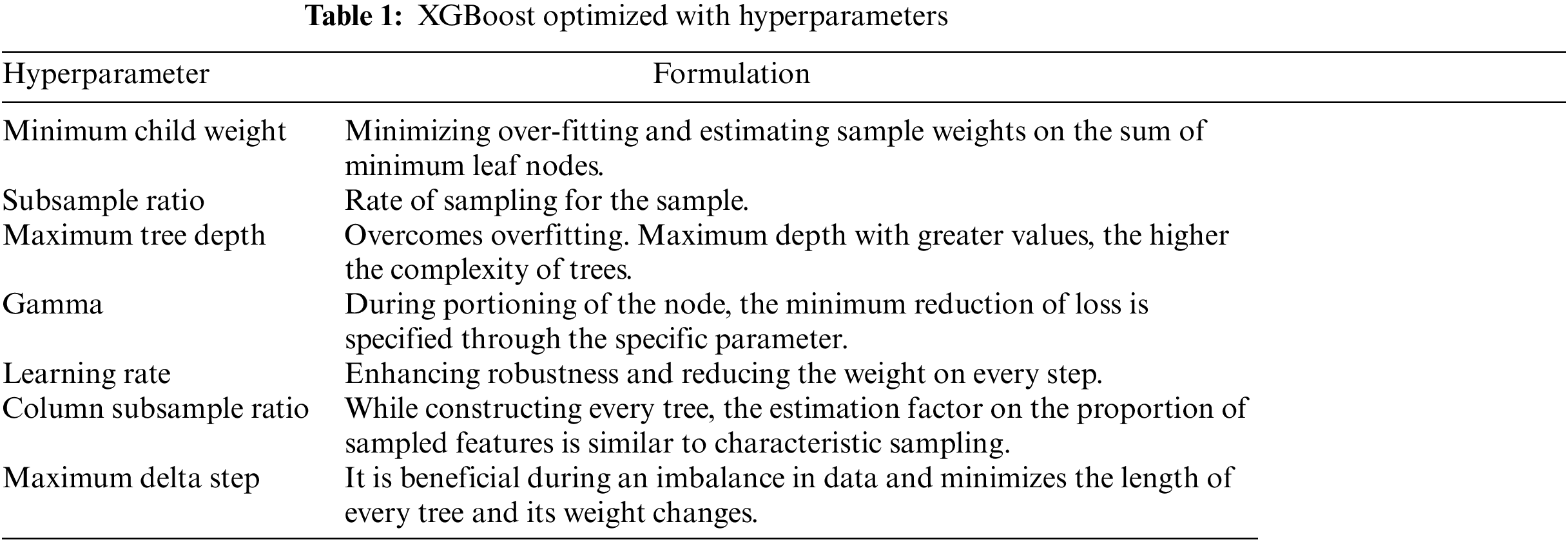
From Table 1, it is clear that the consistency level between the training data and the hyper-parameters determines the model’s efficiency. All the mentioned parameters have been initialized in the search space. They are classified into adaptive populations, achieved through calculating local densities and the distance to particles and determining the particles possessing higher local density. Based on value obtained by the position of particle, data is being validated for prediction of stability. Finally, measured loss function on the validated dataset predicts the fitness function for particles, and logistic loss is expressed as follows:

Losslogistic=log⁡(1+exp⁡(−bp))(17)

in which b is pointing to the actual value and b denotes the prediction value. With the label values 0 and 1, logistic loss is defined as

Losslogistic=1N∑i=1Nbilog(ppi)+(1−bi)log⁡(1−ppi)(18)

Based on the fitness value, particles are classified into ordinary and optimal. Then, based on the particles, information is updated, and the algorithm checks for the termination condition to obtain the optimized value. In addition, depending on the position of particles, the model again repeats calculation of the fitness value and accordingly updates the particle position till it reaches the termination point. Hence, the overall process is depicted in Algorithm 1.

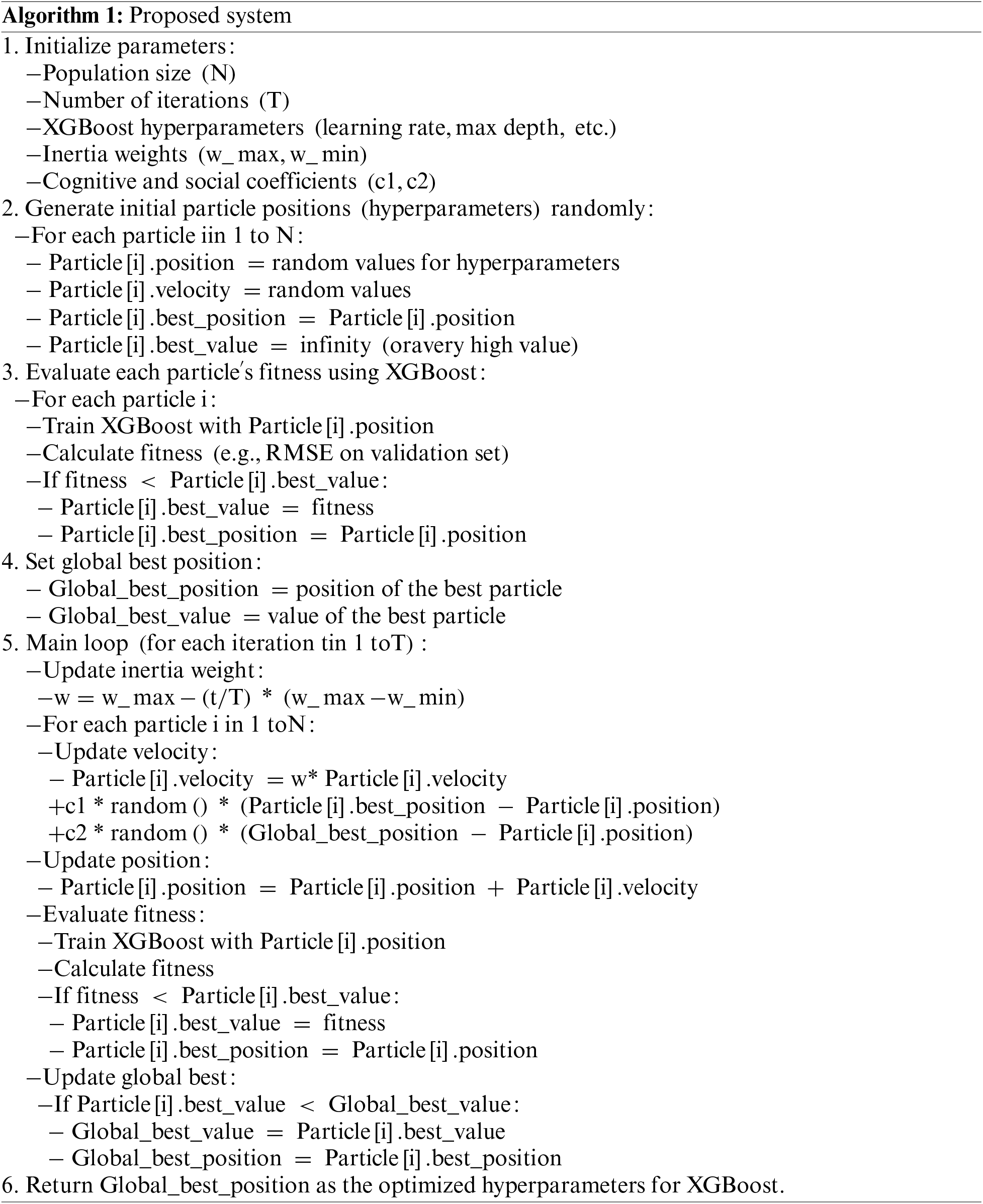
Algorithm 1 employs the PSO to optimize hyperparameters for the XGBoost algorithm. It begins by initializing parameters such as population size, number of iterations, hyperparameters, inertia weights, and cognitive/social coefficients. Each particle, representing a potential solution, is randomly assigned initial positions and velocities, along with tracking its best-known position and fitness value. The fitness of each particle is evaluated by training XGBoost with its hyperparameters and calculating a performance metric like RMSE. The global best position and value are determined based on the best-performing particle. In the main loop, the inertia weight is updated to balance exploration and exploitation, followed by velocity and position updates for each particle based on its personal best and the global best. After re-evaluating fitness and updating the global best as needed, the process iterates until completion. Finally, the algorithm returns the global best position as the optimized hyperparameters for XGBoost, aiming to enhance model performance significantly.

4  Results and Discussion

The performance of the proposed model is evaluated with the prediction rate computed with the regression algorithm. The following section describes the computation result with the internal comparison and comparative analysis with other algorithms to predict the effectiveness of the proposed structure concerning evaluation metrics like RMSE, MSE, and MAPE.

4.1 Dataset Description

The dataset preferred for the proposed algorithm analysis is the Smart Grid Stability Prediction dataset which contains the simulations of stability for a four-node network and contains 10,000 values of observations. Since it is symmetric, the dataset is being augmented as 3 factorials, which results in 60,000 observations with 3 consumers holding 3-consumer nodes. It also provides twelve kinds of predictive attributes and 2 dependent features. The task of regression is performed over the data according to the node structure and predicts the stability.

The predictive features considered in the proposed algorithm are from tau1-tau4, which determines the reaction time taken for every participant with a value within the range from 0.05–1.0. The attribute tau1 denotes supplier-node, and tau2, tau3, and tau4 are consumer-level nodes. Variables p1–p4 determine the nominal power generated (Positive) and consumed as (Negative) by every network participant, with the real value ranging from −2.0 to −0.5 for the consumers (p2–p4). When total consumed power equals total generated power, then p1as the supplier-node = − (p2 + p3 + p4). Attribute g1–g4 exhibits the coefficient of price elasticity for every participant in the network within the range of 0.05–1.00 in which g1 denotes the supplier node and g2–g4 represents the consumer nodes where g refers to gamma. There are two dependent variables, stab and stabf used in analysis where stab signifies the maximum part of differential-equation as a positive value determining the linear instability of the system, and negative stab value points out to the system’s stability. Since features in the dataset are numerical, feature coding is not required. The variable stabf is a categorical label, a binary value representing the stable and unstable nature of the grid. The used dataset is freely available for research in [41].

4.2 Performance Metrics

Performance metrics are specifically employed for enhancing the performances of the model, in which different metrics like RMSE, MSE, MAE, and MAPE are used [42]. Thus, these are some of the performance metrics used for assessing the quality of the model [43].

a) RMSE

It is used to compute the average variance amongst values in the classification and actual values. The RMSE formula is signified in Eq. (19).

RMSE=∑i=1N( acutal−predicted)2/N(19)

b) MSE

It is the measurement of image excellence metric. If the standards are nearer to zero, the metric dimensions have better quality. The formula for MSE is mentioned in Eq. (20).

MSE=1n∑i=1n(Yi−Yi)2(20)

c) Mean Absolute Error (MAE)

It is denoted as the average of the absolute dissimilarity between predicted and actual values. Eq. (21) shows the calculation of MAE.

MAE=∑i=1n|yi−xi|/n(21)

d) MAPE

Mean absolute percentage error measures the average magnitude of error produced by a model, or how far off predictions are on average.

4.3 Experimental Results

The dataset utilized for the proposed work is analyzed, and the computational result obtained from the regression algorithm is illustrated in this section. The experimental outcomes in terms of data reaction time and power balance with stability predictions measured with loss in training also estimate the acquired energy flow at different threshold values, which exhibits the model’s capability in predicting the stability in SG. The variable considered in predictions is observed from the following simulation outcomes depicted in Fig. 4.

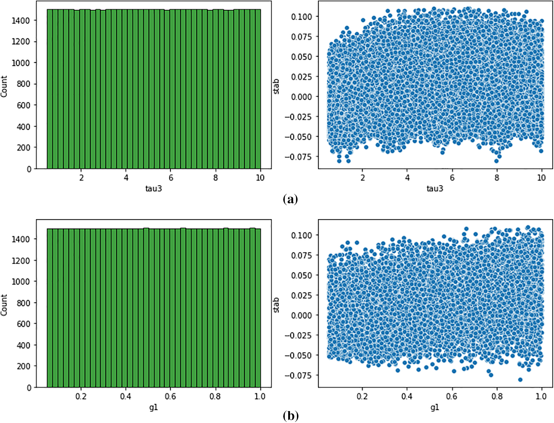
Figure 4: (a) Prediction with tau3 (b) Prediction with g1

Fig. 4a,b exhibits that tau3 as consumer nodes reveals the reaction time taken by participants in the grid, and g1 (gamma) represents the supplier node and observes that it lies within the range of 0.05 to 1.0. The observations infer the efficiency of the prediction model. The dependent variable analysis is illustrated in Fig. 5.

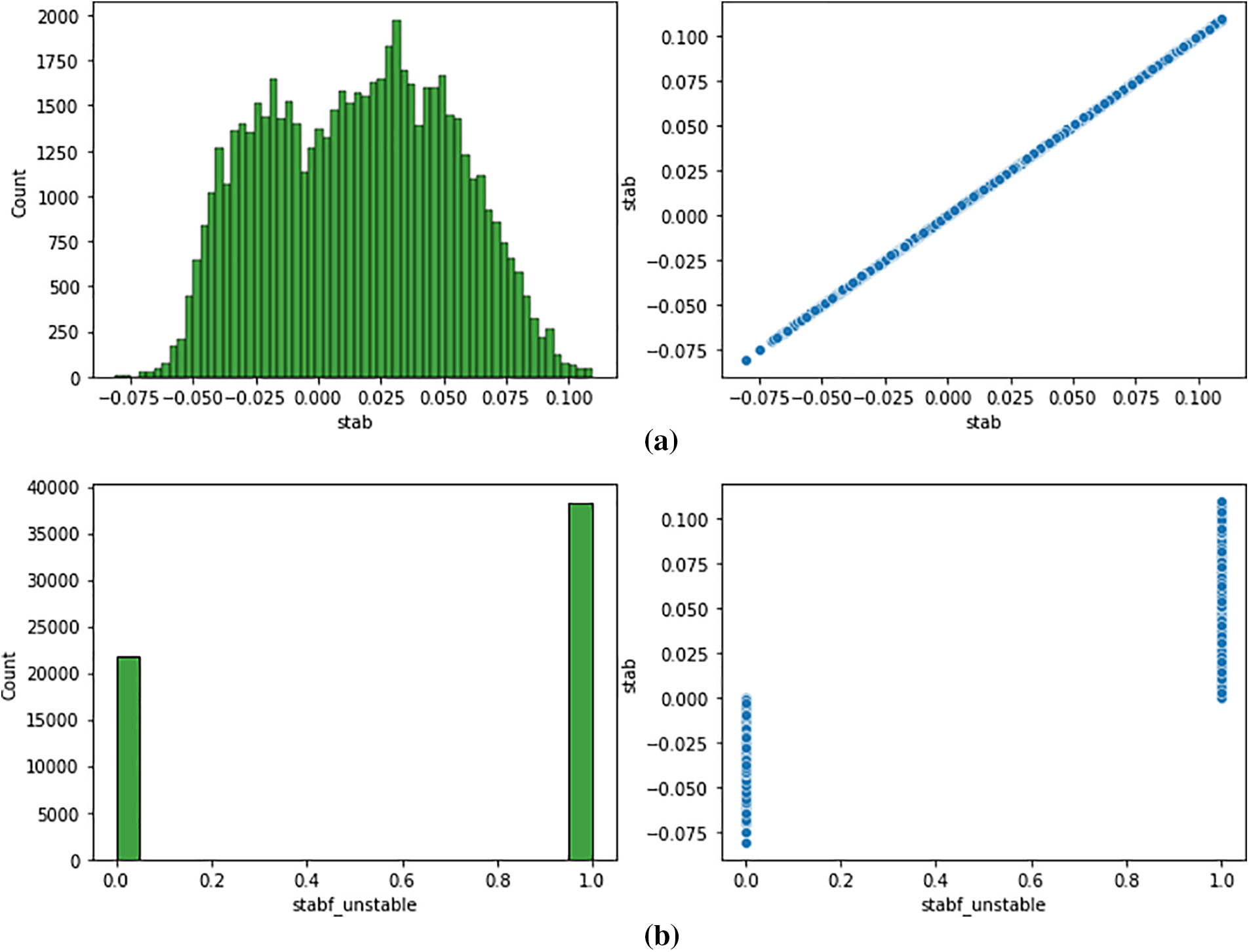
Figure 5: (a) Mapping stable scenario (b) Observations related to unstable nature

From Fig. 5a,b, it is clear that the distributional pattern and relationship with dependent variable stab and stabf is being charted for every feature in the dataset. Since being taken from the simulations performed with a pre-determined range of fixed values, distributions are a uniform normal distribution of skew factors. The output predictions with XGBoost are given below in Fig. 6.

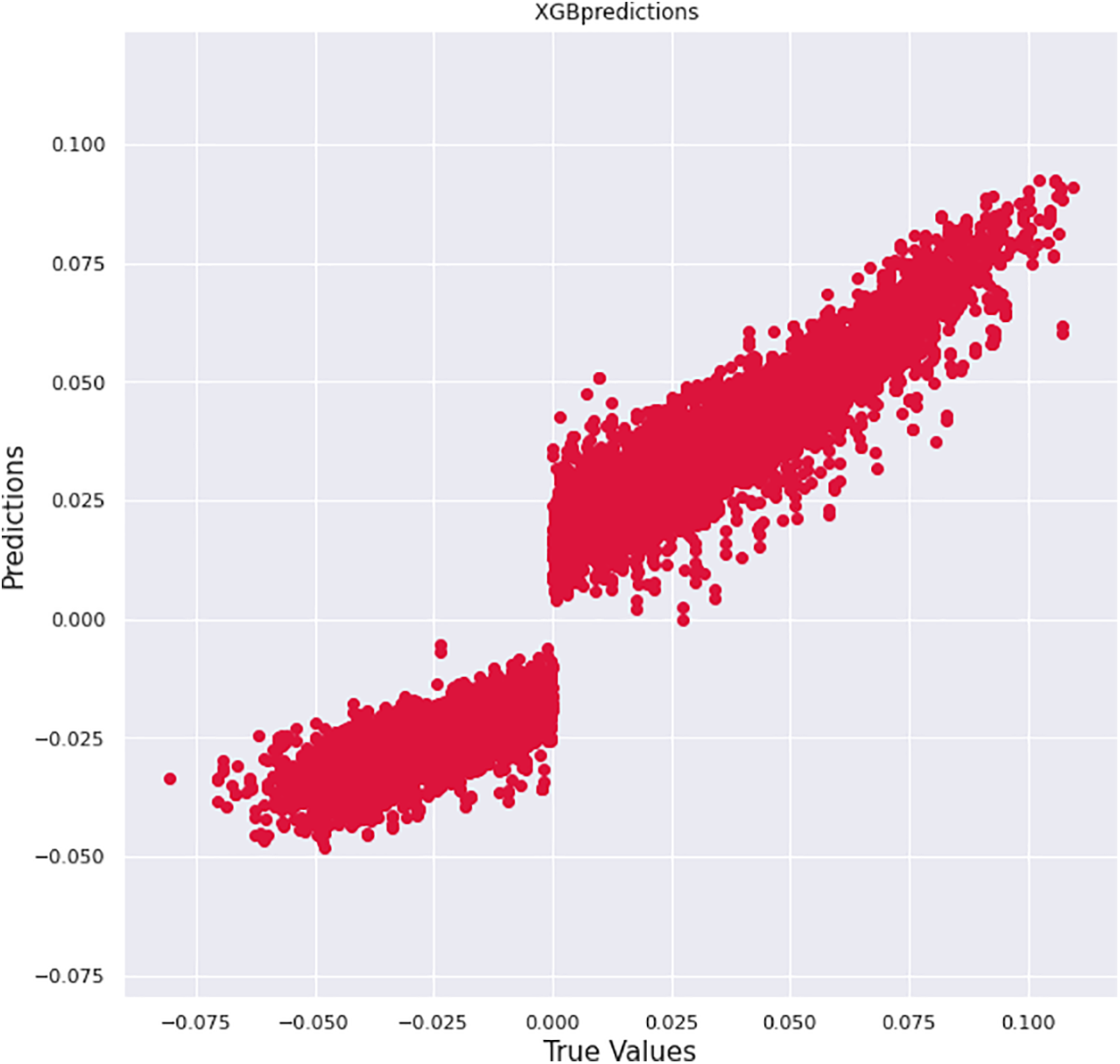
Figure 6: XGBoost predictions

Fig. 6 shows that output predictions from XGBoost with hyperparameter optimization provide extensive distribution and correlation, which explores feasible solution that improves the prediction of grid stability considerably. Factors influencing the stability conditions with different hyperparameters during tuning have been analyzed through simulations, and the correlation observed is determined in Fig. 7.

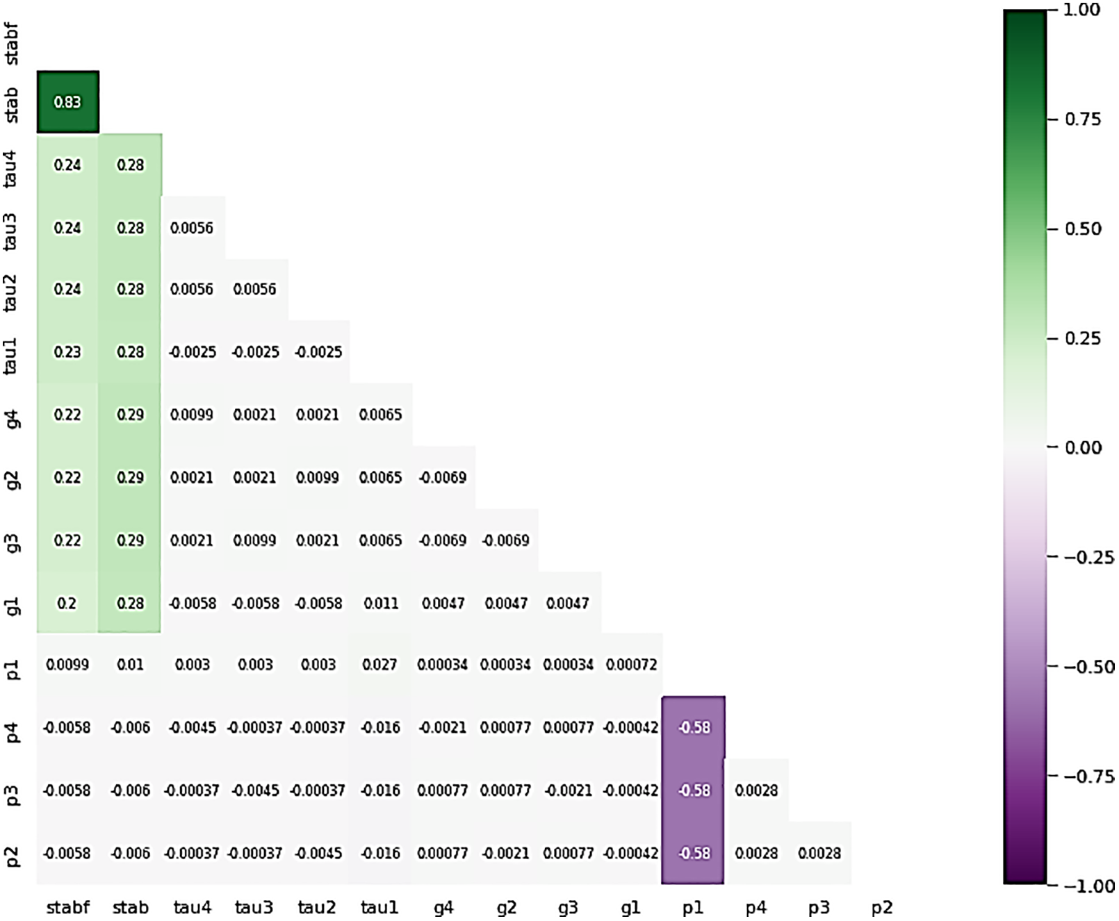
Figure 7: Correlation of predictive and dependent variables

Fig. 7 shows the correlation between every numerical feature and dependent feature to determine the collinearity. For example, the correlation of stab with stabf is found to provide stable points, and a value of 0.83 reinforces the model in prediction. Additionally, the variable p1 is correlated with p2, p3, and p4, which determines the stable value of −0.58, above the average value.

4.4 Performance Analysis

The efficiency of the proposed work is estimated with the evaluation of the system with different performance metrics. The following section describes the analysis made with the experimentation of the system and comparative analysis assessments. Internal evaluation obtained from the regression outcomes is tabulated in Table 2.

From Table 2, it is clear that the proposed algorithm is being evaluated with regression error and estimated concerning MAE of 0.008596, MSE with 0.011312781, RMSE of 0.0106, and MAPE value of 0.0052 which exhibits that minimum loss is being acquired through the model. The graphical illustration of the proposed efficiency is depicted in Fig. 8.

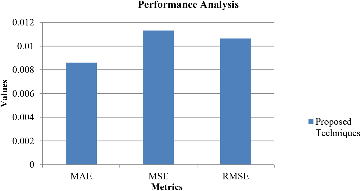
Figure 8: Graphical representation of the proposed algorithm

From Fig. 8, the exploration obtained specifies that the present research is efficient in prediction, as shown through the loss values calculated. The lower loss computed with the proposed work efficiently determines the characteristics of the reaction time, power balance, and non-linearity in energy-stability prediction, which is handled effectively by extracting useful features from the model that gained greater performance in grid-based stability.

4.5 Comparative Analysis

The comparison of the proposed work with the existing algorithm is depicted below in Table 3.

From Table 3, it is clear that the proposed regression algorithm obtains minimum loss compared to existing models like CNN (Convolutional Neural Network), SVR (Support Vector Regression), ESVR (Enhanced Support Vector Regression), and ECNN (Enhanced Convolutional Neural Network), which determines the effectiveness of the proposed regression model. The graphical view of the comparative analysis is depicted in Fig. 9.

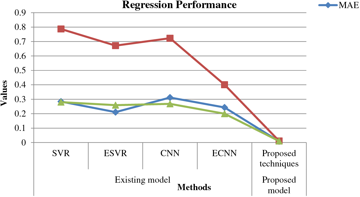
Figure 9: Comparative assessment analysis [44]

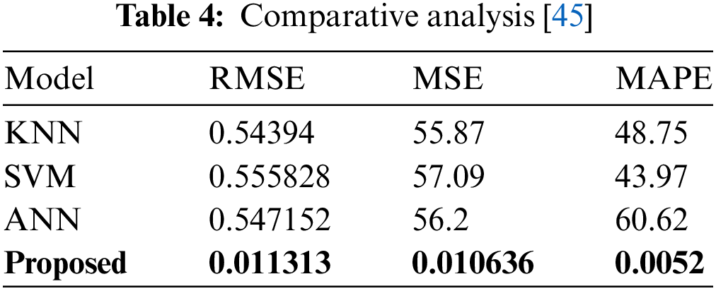
From Fig. 9, it is clear that the proposed regression technique efficiently predicts the stable nature of the grid in the future by determining the effective relationship between the dependent and independent variables. Likewise, Table 4 shows the comparative analysis between various metrics with KNN (K-Nearest Neighbors), SVM (Support Vector Machine), ANN (Artificial Neural Network), and the proposed model.

Table 4 shows that the MAPE, RMSE, and MSE values of the proposed values are less than the existing models, which makes it efficient for predicting the stability of the grid. Therefore, the advantage of the proposed framework is its prediction efficiency and the quality of making effective energy consumption and stability prediction assist in managing smart cities in smart grid in a smother way even during fluctuations in power utilities and maintains the storage and demand effectively. Moreover, it makes the entire system entities regain normal operation during disturbances and maintains stability intact in the grid.

5  Conclusion and Future Recommendation

The proposed regression framework utilized the integration of modified PSO Optimized with XGBoost method by hyperparameters wherein dynamic inertia weight update mechanism was involved in predicting stability in smart grid infrastructure. The regression process performed with the combined approach was evaluated to estimate the model’s efficiency. The regression loss obtained was also compared with other traditional algorithms. As a result, the proposed smart city-based stability prediction was considered efficient since it achieved reduced error values than other existing algorithms. The experimental evaluation performed with the present system found that the enhanced approach attained higher efficacy than other algorithms in terms of MSE, RMSE, and MAE. As future work, the present research can focus on optimizing systems with interpretability and accuracy in providing a decision-support process for many applications involved with smart grid stability control and management. Minimum time and lower computational complexities can also be focused on in the future for effective real-time prediction of stability status. The future work of the proposed model deals with establishing real-time monitoring systems that utilize advanced AI techniques will be essential for proactive stability management. Future work should aim to develop systems that can continuously assess grid conditions and predict potential instabilities before they occur.

Acknowledgement: I want to dedicate this work to Prince Sattam bin Abdulaziz University. Further, I am very much thankful to the reviewers and journal authorities.

Funding Statement: This work was funded by Prince Sattam bin Abdulaziz University project number (PSAU/2023/R/1445).

Author Contributions: The authors confirm contribution to the paper as follows: study conception and design: Adel Binbusayyis, Mohemmed Sha; data collection: Mohemmed Sha; analysis and interpretation of results: Mohemmed Sha, Adel Binbusayyis; draft manuscript preparation: Adel Binbusayyis, Mohemmed Sha. All authors reviewed the results and approved the final version of the manuscript.

Availability of Data and Materials: The code that supports the findings of this study are available from the corresponding author, upon reasonable request.

Ethics Approval: Not applicable.

Conflicts of Interest: The authors declare no conflicts of interest to report regarding the present study.

References

1. Dewangan F, Biswal M, Patnaik B, Hasan S, Mishra M. Smart grid stability prediction using genetic algorithm-based extreme learning machine. In: Electric power systems resiliency. Amsterdam, Netherlands, Elsevier; 2022. p. 149–63. [Google Scholar]

2. Fotopoulou M, Petridis S, Karachalios I, Rakopoulos DJAS. A review on distribution system state estimation algorithms. Appl Sci. 2022;12(21):11073. [Google Scholar]

3. da Cunha GL, Fernandes RA, Fernandes TCC. Small-signal stability analysis in smart grids: an approach based on distributed decision trees. Elect Power Syst Res. 2022;203:107651. doi:10.1016/j.epsr.2021.107651 [Google Scholar] [CrossRef]

4. Breviglieri P, Erdem T, Eken S. Predicting smart grid stability with optimized deep models. SN Comput Sci. 2021;2:1–12. doi:10.1007/s42979-021-00463-5 [Google Scholar] [CrossRef]

5. Petrović N, Al-Azzoni I, Alqahtani A, Alkharj K. Model-driven approach to smart grid stability prediction in Neo4j. In: eNergetics 2021, 2021; Nis, Serbia; p. 299–304. [Google Scholar]

6. Kumar DS, Lau P, Sharma A, Khambadkone A, Srinivasan D. Improvement of transient response in grid-tied photovoltaic systems using virtual inertia. IET Smart Grid. 2021;4(1):1–14. doi:10.1049/stg2.12001 [Google Scholar] [CrossRef]

7. Davari M, Gao W, Blaabjerg F. Analysing dynamics and synthesising a robust vector control for the dc-voltage power port based on the modular multilevel converter in multi-infeed AC/DC smart grids. IET Smart Grid. 2019;2(4):645–58. doi:10.1049/iet-stg.2019.0017 [Google Scholar] [CrossRef]

8. Bodele NA, Shaha R. Design of smart grid of wind power plant by matlab/simulink using PSO. 2022;8(6):27–32. doi:10.46501/IJMTST0806004. [Google Scholar] [CrossRef]

9. Alazab M, Khan S, Krishnan SSR, Pham Q-V, Reddy MPK, Gadekallu TR. A multidirectional LSTM model for predicting the stability of a smart grid. IEEE Access. 2020;8:85454–63. doi:10.1109/ACCESS.2020.2991067 [Google Scholar] [CrossRef]

10. Gorzałczany MB, Piekoszewski J, Rudziński F. A modern data-mining approach based on genetically optimized fuzzy systems for interpretable and accurate smart-grid stability prediction. Energies. 2020;13(10):2559. doi:10.3390/en13102559. [Google Scholar] [CrossRef]

11. Rasheed MB, Qureshi MA, Javaid N, Alquthami T. Dynamic pricing mechanism with the integration of renewable energy source in smart grid. IEEE Access. 2020;8:16876–92. doi:10.1109/ACCESS.2020.2967798. [Google Scholar] [CrossRef]

12. Lu R, Hong SH. Incentive-based demand response for smart grid with reinforcement learning and deep neural network. Appl Energy. 2019;236(8):937–49. doi:10.1016/j.apenergy.2018.12.061. [Google Scholar] [CrossRef]

13. Rodríguez F, Martín F, Fontán L, Galarza A. Very short-term load forecaster based on a neural network technique for smart grid control. Energies. 2020;13(19):5210. doi:10.3390/en13195210. [Google Scholar] [CrossRef]

14. Santos AQ, Monaro RM, Coury DV, Oleskovicz M. A new real-time multi-agent system for under frequency load shedding in a smart grid context. Elect Power Syst Res. 2019;174(12):105851. doi:10.1016/j.epsr.2019.04.029. [Google Scholar] [CrossRef]

15. Djidimbélé R, Ngoussandou B-P, Kidmo DK, Bajaj M, Raidandi D. Optimal sizing of hybrid systems for power loss reduction and voltage improvement using PSO algorithm: case study of Guissia rural grid. Energy Rep. 2022;8:86–95. doi:10.1016/j.egyr.2022.06.093. [Google Scholar] [CrossRef]

16. Shamisa A, Majidi B, Patra JC. Sliding-window-based real-time model order reduction for stability prediction in smart grid. IEEE Trans Power Syst. 2018;34(1):326–37. doi:10.1109/TPWRS.2018.2868850. [Google Scholar] [CrossRef]

17. Hussein SA, Mahmood DY, Numan AH. Loss reduction of transmission lines using PSO-based optimum performance of UPFC. Bull Electr Eng Inform. 2023;12(3):1237–47. doi:10.11591/eei.v12i3.4559. [Google Scholar] [CrossRef]

18. Tesfaye M, Khan B, Mahela OP, Alhelou HH, Gupta N, Khosravy M, et al. Analysing integration issues of the microgrid system with utility grid network. Int J Emerg Electric Power Syst. 2021;22(1):113–27. doi:10.1515/ijeeps-2020-0170. [Google Scholar] [CrossRef]

19. Mehrasa M, Pouresmaeil E, Sepehr A, Pournazarian B, Catalão JP. Control of power electronics-based synchronous generator for the integration of renewable energies into the power grid. Int J Elect Pow Energy Syst. 2019;111(2):300–14. doi:10.1016/j.ijepes.2019.04.016. [Google Scholar] [CrossRef]

20. ZulfiqAr M, Kamran M, Rasheed MB, Alquthami T, Milyani AH. A short-term load forecasting model based on self-adaptive momentum factor and wavelet neural network in smart grid. IEEE Access. 2022;10(20):77587–602. doi:10.1109/ACCESS.2022.3192433. [Google Scholar] [CrossRef]

21. England BS, Alouani AT. Real time voltage stability prediction of smart grid areas using smart meters data and improved Thevenin estimates. Int J Elect Pow Energy Syst. 2020;122(3):106189. doi:10.1016/j.ijepes.2020.106189. [Google Scholar] [CrossRef]

22. Almaghrebi A, Aljuheshi F, Rafaie M, James K, Alahmad M. Data-driven charging demand prediction at public charging stations using supervised machine learning regression methods. Energies. 2020;13(16):4231. doi:10.3390/en13164231. [Google Scholar] [CrossRef]

23. Omar MB, Ibrahim R, Mantri R, Chaudhary J, Ram Selvaraj K, Bingi K. Smart grid stability prediction model using neural networks to handle missing inputs. Sensors. 2022;22(12):4342. doi:10.3390/s22124342. [Google Scholar] [PubMed] [CrossRef]

24. Ge L, Li Y, Yan J, Zhang J, Li X. A multivariate two-stage adaptive-stacking prediction of regional integrated energy system. J Mod Power Syst Clean Energy. 2022;11(5):1462–1479. doi:10.35833/MPCE.2022.000302 [Google Scholar] [CrossRef]

25. Wang Y, Sun S, Chen X, Zeng X, Kong Y, Chen J, et al. Short-term load forecasting of industrial customers based on SVMD and XGBoost. Int J Elect Pow Energy Syst. 2021;129(1):106830. doi:10.1016/j.ijepes.2021.106830. [Google Scholar] [CrossRef]

26. Mishra M, Nayak J, Naik B, Patnaik B. Enhanced memetic algorithm-based extreme learning machine model for smart grid stability prediction. Int Trans Electr Energy Syst. 2022;2022:1–10. doi:10.1155/2022/8038753. [Google Scholar] [CrossRef]

27. Chahal A, Gulia P, Gill NS, Chatterjee JM. Performance analysis of an optimized ANN model to predict the stability of smart grid. Complexity. 2022;2022(1). doi:10.1155/2022/7319010. [Google Scholar] [CrossRef]

28. Geetha R, Ramyadevi K, Balasubramanian M. Prediction of domestic power peak demand and consumption using supervised machine learning with smart meter dataset. Multimed Tools Appl. 2021;80(13):19675–93. doi:10.1007/s11042-021-10696-4. [Google Scholar] [CrossRef]

29. Senyuk M, Safaraliev M, Kamalov F, Sulieman H. Power system transient stability assessment based on machine learning algorithms and grid topology. Mathematics. 2023;11(3):525. doi:10.3390/math11030525. [Google Scholar] [CrossRef]

30. Kofinas P, Dounis A, Vouros G. Fuzzy Q-Learning for multi-agent decentralized energy management in microgrids. Appl Energy. 2018;219(1):53–67. doi:10.1016/j.apenergy.2018.03.017. [Google Scholar] [CrossRef]

31. Sufyan MAA, Zuhaib M, Anees MA, Khair A, Rihan M. Implementation of PMU-based distributed wide area monitoring in smart grid. IEEE Access. 2021;9:140768–78. doi:10.1109/ACCESS.2021.3119583. [Google Scholar] [CrossRef]

32. Zhang WJ. Forecasting and management in smart grid with artificial intelligence. National University of Singapore: Singapore; 2020. [Google Scholar]

33. Chou J-S, Hsu S-C, Ngo N-T, Lin C-W, Tsui C-C. Hybrid machine learning system to forecast electricity consumption of smart grid-based air conditioners. IEEE Syst J. 2019;13(3):3120–8. doi:10.1109/JSYST.2018.2890524. [Google Scholar] [CrossRef]

34. Wood DA. Predicting stability of a decentralized power grid linking electricity price formulation to grid frequency applying an optimized data-matching learning network to simulated data. Technol Econ Smart Grids Sustain Energy. 2020;5(1):3. doi:10.1007/s40866-019-0074-0. [Google Scholar] [CrossRef]

35. Dong J. Peak load ensemble prediction and multi-agent reinforcement learning for DER demand response management in smart grids. 2022. Available from: https://knowledgecommons.lakeheadu.ca/handle/2453/4944. [Accessed 2024]. [Google Scholar]

36. Vanfretti L, Arava VN. Decision tree-based classification of multiple operating conditions for power system voltage stability assessment. Int J Elect Pow Energy Syst. 2020;123(11):106251. doi:10.1016/j.ijepes.2020.106251. [Google Scholar] [CrossRef]

37. Ibrar M, Hassan M, Shaukat Dar K, Mahboob Alam T, Khurshid SK, Hameed I, et al. A machine learning-based model for stability prediction of decentralized power grid linked with renewable energy resources. Wirel Commun Mob Comput. 2022;2022:1–15. doi:10.1155/2022/2697303 [Google Scholar] [CrossRef]

38. Oh S, Yoon J, Choi Y, Jung Y-A, Kim J. Genetic algorithm for the optimization of a building power consumption prediction model. Electronics. 2022;11(21):3591. doi:10.3390/electronics11213591. [Google Scholar] [CrossRef]

39. Mostafa N, Ramadan HSM, Elfarouk O. Renewable energy management in smart grids by using big data analytics and machine learning. Mach Learn with Appl. 2022;9(5):100363. doi:10.1016/j.mlwa.2022.100363. [Google Scholar] [CrossRef]

40. Cebekhulu E, Onumanyi AJ, Isaac SJ. Performance analysis of machine learning algorithms for energy demand-supply prediction in smart grids. Sustainability. 2022;14(5):2546. doi:10.3390/su14052546. [Google Scholar] [CrossRef]

41. Tiwari S, Jain A, Yadav K, Ramadan R. Machine learning-based model for prediction of power consumption in smart grid. Int Arab J Inf Technol. 2022;19(3):323–9. doi:10.34028/iajit. [Google Scholar] [CrossRef]

42. Garg S, Krishnamurthi R. A CNN encoder decoder LSTM model for sustainable wind power predictive analytics. Sustain Comput: Inform Syst. 2023;38:100869. doi:10.1016/j.suscom.2023.100869 [Google Scholar] [CrossRef]

43. Sina LB, Secco CA, Blazevic M, Nazemi KJE. Hybrid forecasting methods—a systematic review. Electronics. 2023;12(9):2019. doi:10.3390/electronics12092019 [Google Scholar] [CrossRef]

44. Zahid M, Ahmed F, Javaid N, Abbasi RA, Zainab Kazmi HS, Javaid A, et al. Electricity price and load forecasting using enhanced convolutional neural network and enhanced support vector regression in smart grids. Electronics. 2019;8(2):122. doi:10.3390/electronics8020122 [Google Scholar] [CrossRef]

45. Shapi MKM, Ramli NA, Awalin LJ. Energy consumption prediction by using machine learning for smart building: case study in Malaysia. Develop Built Environ. 2021;5:100037. doi:10.1016/j.dibe.2020.100037 [Google Scholar] [CrossRef]