iconOpen Access

ARTICLE

Global Piecewise Analysis of HIV Model with Bi-Infectious Categories under Ordinary Derivative and Non-Singular Operator with Neural Network Approach

by Ghaliah Alhamzi1, Badr Saad T. Alkahtani2, Ravi Shanker Dubey3, Mati ur Rahman4,5,*

1 Department of Mathematics and Statistics, College of Science, Imam Mohammad Ibn Saud Islamic University (IMSIU), Riyadh, 13318, Saudi Arabia
2 Department of Mathematics, College of Science, King Saud University, Riyadh, 11989, Saudi Arabia
3 Department of Mathematics, Amity School of Applied Sciences, Amity University Rajasthan, Jaipur, 302002, India
4 School of Mathematical Sciences, Jiangsu University, Zhenjiang, 212013, China
5 Department of Computer Science and Mathematics, Lebanese American University, Beirut, 13-5053, Lebanon

* Corresponding Author: Mati ur Rahman. Email: email

(This article belongs to the Special Issue: Innovative Applications of Fractional Modeling and AI for Real-World Problems)

Computer Modeling in Engineering & Sciences 2025, 142(1), 609-633. https://doi.org/10.32604/cmes.2024.056604

Abstract

This study directs the discussion of HIV disease with a novel kind of complex dynamical generalized and piecewise operator in the sense of classical and Atangana Baleanu (AB) derivatives having arbitrary order. The HIV infection model has a susceptible class, a recovered class, along with a case of infection divided into three sub-different levels or categories and the recovered class. The total time interval is converted into two, which are further investigated for ordinary and fractional order operators of the AB derivative, respectively. The proposed model is tested separately for unique solutions and existence on bi intervals. The numerical solution of the proposed model is treated by the piece-wise numerical iterative scheme of Newtons Polynomial. The proposed method is established for piece-wise derivatives under natural order and non-singular Mittag-Leffler Law. The cross-over or bending characteristics in the dynamical system of HIV are easily examined by the aspect of this research having a memory effect for controlling the said disease. This study uses the neural network (NN) technique to obtain a better set of weights with low residual errors, and the epochs number is considered 1000. The obtained figures represent the approximate solution and absolute error which are tested with NN to train the data accurately.

Keywords


1  Introduction

Viruses of HIV lie and transmit both in classical and modern world contents having various rates of infection. Among the sources of spreading of the said diseases from one man to another are through sexual meetings, used needles re-usages, drug usage, inherited through the mother, and by un-tested blood donations or transfusions. For stabilizing HIV infection transmission, there are various approaches including need-based HIV testing, usage of condoms during sex, circumcisions, usage of vaginal microbicides and antire-troviral (ARV) drug. To date, no cure or vaccination for HIV has been successfully discovered [1].

HIV infection is among the badly killing diseases, causing thousands of deaths all over the globe. Nearly thirty-eight million humans all over the world suffered from HIV in the year of 2019. After that, the virus has spread to each country of the globe. According to the statistics of the Health Ministry about 21,500 men were suffering from HIV in the African country of Morocco [1]. Among them, 6000(22%) were ignorant of their infection. In 2019 about 850 novel HIV testing in Morocco, 33% were aged 15–25. This analysis also gives 300 deaths data. In more detail, 67% of novel cases occur in highly risky chain populations. About 70.7% of women are tested positively due to their husbands. Statistical data implies a low percentage of HIV infection in the country of Morocco in common lie population, (0.08%),1.7% are tested females working in different fields, 5.9% on mean are the homo-sexuals, 7.1% on mean are those taking drugs by injections. Some territories of the country numbered about 65% of all infections, namely Sous-Massa (26%), Marrakech-Safi (20%) and Casablanca-Settat (20%) [1].

In dealing with such infection, one of the significant tools is mathematical modeling whose benefits are to provide an esteemed prediction and feedback of any infection transmission whose viruses are contagious and invisible. Mathematical models of HIV are constructed by the scientific approval, given by analyzers, physicians and pharmacists along with the limit of spreading of the virus. So different HIV systems have been investigated by many authors [25]. Researchers have examined various models by applying different methodologies and explored the behaviors of each class and comparisons to real data [69]. Fractional calculus can be a useful technique in HIV disease modeling to capture the complex dynamics of the illness, particularly in areas where standard models are inadequate. It does, however, also provide new difficulties about the interpretation and complexity of mathematics [1013]. Silva et al. [12] have considered an epidemiological system of HIV/AIDS transmissions including Pre-exposed Prophylaxis. In the same fashion, Li et al. [5] made a susceptible exposure in the Latent stage infection (SEI) level to draw the evolution of HIV. One of the Vivo deterministic problems has been discussed by Ngina et al. [7]. Shirazian et al. [11] have considered a mathematical method applied to express mathematically the procedure for medical tests and seeing the infection of HIV/AIDS.

The scholars have proposed a continuous system of five agents SI1I2QR for discussion of the interaction among the populations having HIV/AIDS. Here S,I1,I2,Q,R are the cases of susceptible peoples, Infectious peoples stage 1, infectious peoples stage 2, Infectious peoples who are hospitalized and recoverable individuals, respectively [1]. The said model is given below:

dS(t)dt=ΔuS(β1I1+β2I2)SdI1(t)dt=β1I1S+δ2I2(δ1+γ1+u+σ1)I1dI2(t)dt=β2I2S+δ4Q+δ1I1(γ2+δ2+δ3+u+σ2)I2dQ(t)dt=δ3I2(γ3+δ4+u+σ3)QdR(t)dt=σ1I1+σ2I2+σ3QuRS(0)=S0,I1(0)=I10,I2(0)=I20,Q(0)=Q0,R(0)=R00.(1)

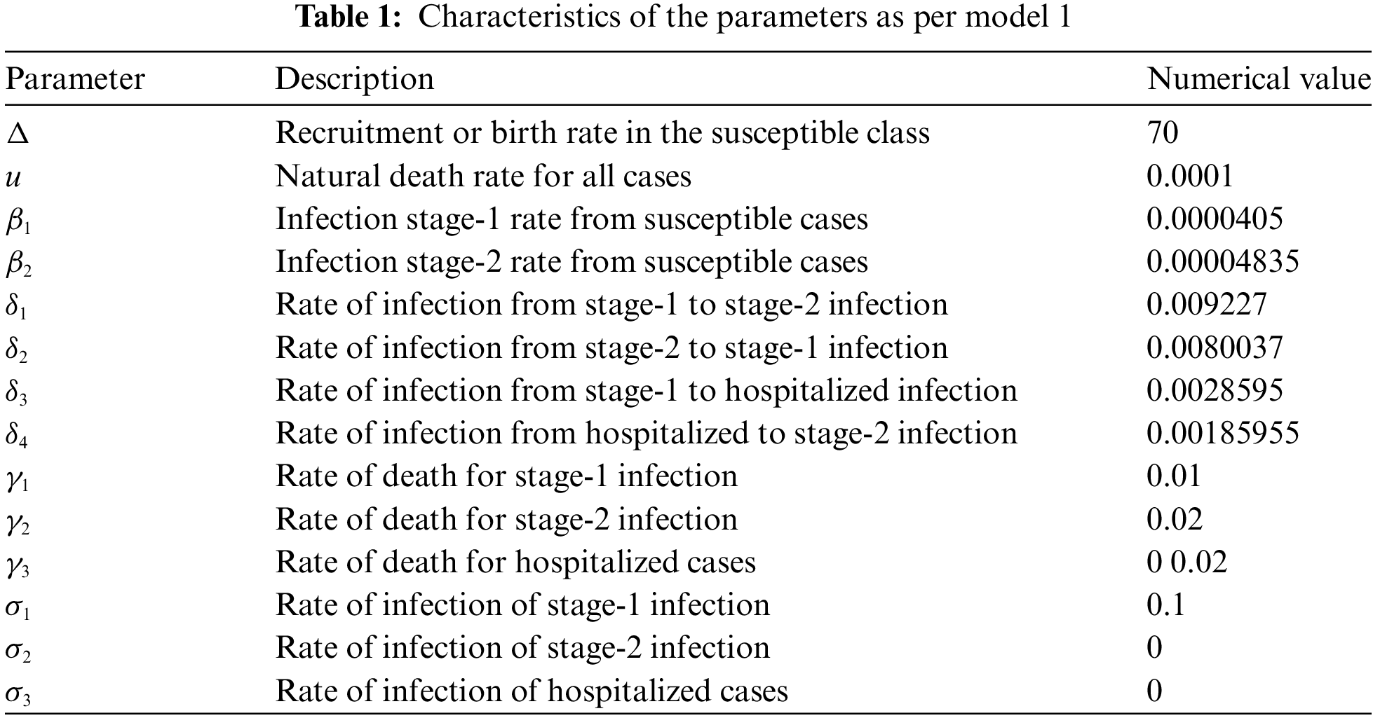
The used parameters are defined in Table 1 [1] along with numerical values.
images

Many sorts of derivatives have been developed in multiple attempts to understand cross-over dynamics and overcome discontinuities. These comprise fractal-fractional derivatives, derivatives of fractional order whose kernels show singularity and non-singularity, and other special cases of derivatives [1417]. These methods, which offer sophisticated instruments for capturing the intricacies present in such dynamic processes, have all been designed to address particular facets of the behavior of the system [1822]. These various derivative formulations enable a more sophisticated analysis of cross-over dynamics, allowing for the exploration of system transitions between multiple states or phases. Derivatives make it possible to model complicated, real-world processes more accurately and adaptably by taking into account both continuity and discontinuity [2326]. This is particularly important in the domain of disease modeling, where a precise understanding of the dynamics of transitions, such as the HIV’s transition from latency to active infection, can result in more accurate forecasts and more potent interventions [27,28]. For analysis of the randomness or probabilistic in the scheme of stochastic equations having more real findings but up to now the cross-over dynamical behavior has not been investigated. Such behaviors are found in most infection models, like the heat flow, fluid dynamics, and many of the complex geometrical problems [22,29,30]. In fractional derivatives, the exponential and Mittag-Leffler mapping are not used to compute the time of crossover dynamics. Hence to treat such models, one of the novel schemes of piece-wise derivatives and antiderivatives has been formulated in [31]. A comprehensive framework incorporating global and classical piecewise derivatives was built by the concept’s authors. These derivatives were developed to model complicated systems, namely the dynamics of HIV infection. Keeping in view the said aspects, we will also discuss the said problem for at least one solution, uniqueness of solution, numerical solution, and stability analysis in the sense of classical and Atangana-Baleanu (AB) piecewise derivative. Further, such kind of operators are different and better than the other fractional operators. It removes the discontinuity on the whole interval by converting it into a sub-interval, it describes the crossover dynamics, AB operator has the non-singular kernel which removes the singularity of the given domain, it quickly gains the stability of any dynamical system on small fractional order, is more generalized than classical and other fractional operators. Moreover, the neural network (NN) approach is utilized and find different data sets for the considered model and the comparison of fractional and NN as well. The Eq. (1) is expressed in piece-wise derivative in the sense of classical and non-singular kernel operator as under.

D0ψ0POAB(S)(t)=ΔuS(β1I1+β2I2)SD0ψ0POAB(I1)(t)=β1I1S+δ2I2(δ1+γ1+u+σ1)I1D0ψ0POAB(I2)(t)=β2I2S+δ4Q+δ1I1(γ2+δ2+δ3+u+σ2)I2D0ψ0POAB(Q)(t)=δ3I2(γ3+δ4+u+σ3)QD0ψ0POAB(R)(t)=σ1I1+σ2I2+σ3QuR,t[0,T], 0tt1, t1tt2,(2)

where POAB is for piece-wise ordinary and AB derivative in two sub-intervals of [0,T]. In more simplest form we can write Eq. (2) under

D0ψ0POAB(S(t))={Dt0O(S(t))=ddtF1(S,t),0<tt1,Dtψ0AB(S(t))=ABF1(S,t)t1<tt2,D0ψ0POAB(I1(t))={Dt0O(I1(t))=ddtF2(I1,t),0<tt1,Dtψ0AB(I1(t))=ABF2(I1,t),t1<tt2,D0ψ0POAB(t))={Dt0O(I2(t))=ddtF3(I2,t),0<tt1,Dtψ0AB(I2(t))=ABF3(I2,t),t1<tt2,D0ψ0POAB(Q(t))={Dt0O(Q(t))=ddtF4(Q,t),0<tt1,Dtψ0AB(Q(t))=ABF4(Q,t),t1<tt2,D0ψ0POAB(R(t))={Dt0O(R(t))=ddtF5(R,t),0<tt1,Dtψ0AB(R(t))=ABF5(R,t),t1<tt2,(3)

where Dt0O and Dtψ0AB are ordinary and AB fractional derivative respectively and Fi from i=1,2,3,4,5 is for left side of Eq. (2).

1.1 Basis Properties of the Model

For any epidemiological problem, most of the authors assume that the total size of population N(t) is constant, in the rest of the paper, i.e.,

S+I1+I2+Q+R=N(t)t0

The transfer diagram may also be seen in [1].

Lemma 1.1. The set

Ξ={S,I1,I2,Q,R}>0R5andS+I1+I2+Q+R<Δu

is bounded in positive feasible region.

Proof. Adding all the five agents of Eq. (2) as follows:

S+I1+I2+Q+R=N(t)t0,

or

Dtψ0POAB(N(t))=Δu(S+I1+I2+Q+R)γ1I1γ2I2γ3QΔuN(t)

Dtψ0POAB(N(t))+uN(t)Δ.

On application of piece-wise integration we get

It0ON(t){N(0)eut+Δu(1eut),0<tt1,N(t1)+1ψABψN(t)+ψABψΓψt1t(tτ)ψ1N(τ)d(τ)t1<tt2.

In the first interval if t1 is large then N(t)Δut0 and in the second interval if t2, then N(t)Δu,t10. Hence for both cases the system is bounded in the feasible region. ■

Lemma 1.2. If the initial values of all the agent of the (2) is non-negative, i.e., S(0)0,I1(0)0,I2(0)0,Q(t)0,R(0)0 then the solution of problem (2) for each quantity will be positive for t1>0 and t2>0.

Proof. The proof can be seen in [1]. ■

The free equilibrium point for the model (2) is E0=(S0,I10,I20,Q0,R0)=(Δu,0,0,0,0).

The Basic reproduction number for (2) [1] is

R0=ζ2((β1P2+β2P1)+(β1P2β2P1)+4β1β2γ1γ2),

where P1=δ1+γ1+u+σ1,P2=δ2+δ3+γ2+u+σ2 and ζ=1P1P2γ1γ2. Further if R0<1 on equilibrium point then problem (2) is locally asymptotically stable and unstable if R0>1.

R0<1 means that any infected population may transfer the disease to less than one new infected individual, which implies that HIV infection does not spread in the population.

R0>1 means that any infected population may transfer the disease to more than one new infected individual, which implies that HIV infection spreads in the population.

2  Basic Results

Now, in the next part of the article, we provide a few background definitions of the Caputo operator of derivative and integration along with the piecewise derivative concept.

Definition 2.1. The AB derivative of a function Ψ(t) under the condition Ψ(t)1(0,τ) is defined as follows:

Dtψ0AB(Ψ(t))=AB(ψ)1ψ0tddτΨ(τ)Eψ[ψ1ψ(tτ)ψ]dτ.(4)

While the integral can be written as

Dtψ0ABΨ(t)=1ψAB(ψ)Ψ(t)+ψAB(ψ)Γ(ψ)0t(tτ)ψ1Ψ(τ)dτ.(5)

Definition 2.2. Choosing ω(t) be differentiable and g(t) is increasing function then classical piece-wise derivative [31] can be given as

It0OΨ(t)={Ψ(t),0<tt1,Ψ(t)g(t)t1<tt2=T,

and the integration is

It0OΨ(t)={0tΨ(τ)dτ,0<tt1,t1tΨ(τ)g(τ)d(τ) t1<tt2,

here It0OΨ(t) and Dt0OΨ(t) are for ordinary derivative and integration for 0<tt1 and global derivative integration for t1<tt2

Definition 2.3. Let Ψ(t) be differentiable then ordinary and fractional piece-wise derivative [31] is defined as

Dtψ0OΨ(t)={Ψ(t),0<tt1,Dtψ0ABΨ(t) t1<tt2,

while the integration can be

It0OΨ(t)={0tΨ(τ)dτ,0<tt1,1ψABψΨ(t)+ψABψΓψt1t(tτ)ψ1Ψ(τ)d(τ) t1<tt2,

here Dtψ0OΨ(t) and It0OΨ(t) are for ordinary derivative and integration for 0<tt1 and AB fractional derivative integration for t1<tT2.

Lemma 2.1. The solution of piece-wise derivable equation

Dtψ0OABΨ(t)=F(t,Ψ(t)),0<r1

is

Ψ(t)={Ψ0+0tΨ(τ)dτ, 0<tt1Ψ(t1)+1ψABψΨ(t)+ψABψΓψt1t(tτ)ψ1Ψ(τ)d(τ), t1<tt2.

3  Existence and Uniqueness

This section will evaluate whether the piece-wise derivable problem under consideration has a unique solution and whether it exists or not. Based on the information provided in Lemma 2.1, we write the system (2) for this, and we further describe it as follows:

Dtψ0POABΨ(t)=F(t,Ψ),0<ψ1

is

Ψ(t)={Ψ0+0tF(s,Ψ(s))ds, 0<tt1Ψ(t1)+1ψABψΨ(t)+ψABψΓψt1t(ts)ψ1Ψ(s)ds, t1<tt2,(6)

where

Ψ(t)={S(t)I1(t)I2(t)Q(t)R(t), Ψ0={S0I10I20Q0R0, Ψt1={S(t1)I1(t1)I2(t1)Q(t1)R(t1), F(t,Ψ(t))={F1={ddtF1(S,t)F1AB(S,t)F2={ddtF2(I1,t)F2AB(I1,t)F3={ddtF3(I2,t)F3AB(I2,t)F4={ddtF4(Q,t)F4AB(Q,t)F5={ddtF5(R,t)F5AB(R,t)(7)

Consider >t2t>t1>0 with closed norm space as G1=C[0,T] having norm

Ψ=maxt[0,T]|Ψ(t)|.

For the required result, we take the growth condition on the non-linear operator as

(A1) LΨ>0; G,Ψ¯E we have

|F(t,Ψ)F(t,Ψ¯)|LF|ΨΨ¯|,

(A2) CF>0 & MF>0,;

|F(t,Ψ(t))|CF|Ψ|+MF.

Theorem 3.1. Let F be a piece-wise continuous mapping on sub-interval 0<tt1 and t1<tt2 on [0,T], also satisfying (A2), then piece-wise derivative (3) has at least one solution on each sub-interval.

Proof. Let us assume a closed subset in both sub-intervals of 0,T as E of B by using the Schauder fixed point theorem

E={ΨB:|ΨR1,2, R>0},

Next, let us suppose an operator T:EE and applying (6) as

T(Ψ)={Ψ0+0tF(τ,Ψ(τ))dτ, 0<tt1Ψ(t1)+1Γ(ψ)0t1F(τ,Ψ(τ))(tτ)ψ1dτ, t1<tt2Ψ(t1)+1ψAB(ψ)F(t,Ψ(t))+ψAB(ψ)Γ(ψ)t1t(tτ)ψ1F(τΨ(τ))d(τ),  t1<tt2.(8)

On some ΨE, we follows as

|T(Ψ)(t)|{|Ψ0|+0t1|F(τ,Ψ(τ))|dτ,|Ψ(t1)|+|1ψAB(ψ)F(t,Ψ(t))+ψAB(ψ)Γ(ψ)t1t(tτ)ψ1|F(τΨ(τ))d(τ),{|Ψ0|+0t1[CF|Ψ|+MG]dτ,|Ψ(t1)|+1ψAB(ψ)[CF|Ψ|+MF+ψAB(ψ)Γ(ψ)t1t(tτ)ψ1[CF|Ψ|+MF]dτ,{|Ψ0|+t1[CF|Ψ|+MF]=R1, 0<tt1,|Ψt1|+1ψAB(ψ)[CF|Ψ|+MF]+ψ(TT)ψAB(ψ)Γψ+1[CF|Ψ|+MF]dτ=R2, t1<tt2,{R1, 0<tt1,R2, t1<tt2.

The final equation suggests that T(E)E since ΨE. It follows that T is closed and complete. Moving forward, we will assume perfect continuity. Specifically, we will use tm<tn[0,t1] as the first interval of the classical derivative notion.

|T(Ψ)(tn)T(Ψ)(tm)|=|0tnF(τ,Ψ(τ))dτ0tmF(τ,Ψ(τ))dτ|0tn|F(τ,Ψ(τ))|dτ0tm|F(τ,Ψ(τ))|dτ[0tn(CF|Ψ|+MF)0tm(CF|Ψ|+MF)(CFΨ+MF)[tntm].(9)

Next from (9), we obtain tmtn, then

|T(Ψ)(tn)T(Ψ)(tm)|0,as tmtn.

Thus, in the interval [0,t1], T is equi-continuous. Next, we take the other AB sense interval ti,tj[t1,T] as

|𝒯(Ψ)(tj)𝒯(Ψ)(ti)|=|1ψAB(ψ)F(t,Ψ(t))+ψAB(ψ)Γ(ψ)t1tj(tjτ)ψ1F(τ,Ψ(τ))dτ,1ψAB(ψ)F(t,Ψ(t))+(ψ)AB(ψ)Γ(ψ)t1ti(tiτ)ψ1F(τ,Ψ(τ))dτ|ψAB(ψ)Γ(ψ)t1ti[(tiτ)ψ1(tjτ)ψ1]|F(τ,Ψ(τ))|dτ+ψAB(ψ)Γ(ψ)titj(tjτ)ψ1|F(τ,Ψ(τ))|dτψAB(ψ)Γ(ψ)[t1ti[(tiτ)ψ1(tjψ)ψ1]dτ+titj(tjτ)ψ1dτ](CF|Ψ|+MF)ψ(CHΨ+MH)AB(τ)Γ(ψ+1)[tjψtiψ+2(tjti)ψ].(10)

Further from (10) we get tmtn, then

|T(Ψ)(tn)T(Ψ)(tm)|0,as tmtn.

Therefore, in the interval [t1,t2], T is equi-continuous. It follows that T is an equi-continuous mapping. The Arzelá-Ascoli Theorem shows that operator T is limited, uniform, and continuous. There is at least one solution to the piecewise derivable problem (3) on each subinterval, according to Schauder’s fixed point theorem. ■

Theorem 3.2. If T is a contraction operator, then the suggested piece-wise model has a unique root with condition (A1).

Proof. As previously, given a piece-wise continuous mapping T:EE, let Ψ and Ψ¯E on [0,t1] be understood as

T(Ψ)T(Ψ¯)=maxt[0,t1]|0t1F(τ,Ψ(τ))dτ0t1F(τ,Ψ¯(τ))dτ|t1LFΨΨ¯.(11)

From (11), we have

T(Ψ)T(Ψ¯)t1LFΨΨ¯.(12)

It follows that T is contraction. In summary, the problem under consideration has a unique solution inside the specified subinterval according to the outcome of the Banach contraction theorem. Additionally, in the context of the AB derivative, for the second sub-interval t[t1,t2] as

T(Ψ)T(Ψ¯)1ψAB(ψ)LFΨΨ¯+ψ(TTψ)AB(ψ)Γ(ψ+1)LFΨΨ¯.(13)

or

T(Ψ)T(Ψ¯)LF[1ψAB(ψ)+ψ(TT)ψAB(ψ)Γ(ψ+1)]ΨΨ¯.(14)

The presented problem, therefore, has a unique solution in the second sub-interval according to the Banach contraction theorem since T is contraction. Consequently, each sub-interval of the piecewise derivable model has a unique solution according to Eqs. (12) and (14). ■

Ulam Hyers Stability

To obtain the Ulam-Hyers stability for the proposed model, we need to prove that a small perturbed term in the starting condition or the parameters of the system implies small perturbations in the solution of the system. It can be achieved by deriving that the operator T is Lipschitz continuous w.r.t the starting conditions or any of the parameters of the system.

Definition 3.1. The proposed model (2) is called Ulam-Hyers stable, if for all N>0, then the following inequality holds true.

|DtψPOABCΨ(t)F(t,Ψ(t))|<N,tT.(15)

Let we have a unique solution Ψ¯Y that is constant A>0,

||ΨΨ¯||YAN,forall,tT.(16)

Next, if we chose an increasing operator U:[0,)R+, the inequality above can be written as under:

||ΨΨ¯||ZAU(N),for each,tT.

If U(0)=0, then the final solution is general Ulam-Hyers (G-H-U) stable.

Remark 1. Assume that an operator UC(𝒯) is independent of ΨW and holds U(0)=0, then

|U(t)|N,tTDtψPOABCΨ(t)=F(t,Ψ(t))+U(t),tT.

Lemma 3.1. Let the mapping

Dψt0POABCΨ(t)=F(t,Ψ(t)),0<ψ1.(17)

The solution of (17) is

Ψ(t)={Ψ0+0tF(z,Ψ(z))dz, 0<tt1Ψ(t1)+1ψAB(ψ)F(t,Ψ(t))+ψAB(ψ)Γ(ψ)t1t(tz)ψ1F(z,Ψ(z))dz,t1<tT,(18)

||F(Ψ)F(Ψ¯)||{Ψ0+t1[CF|Ψ|+MF]N,t(0,t1][(1ψ)Γ(ψ)+(t2ψ)AB(ψ)Γ(ψ)]N=ΛN,t[t1,t).(19)

Theorem 3.3. Lemma (3.1) implies that if LFtψΓ(ψ)<1, then the solution to model (3) is Hyers-Ulam stable as well as G-H-U stable.

Proof. If Ψ𝒲 is a solution of (3) and Ψ¯𝒲 is also a unique solution of (3), then we have

Case: 1 for t(0,t], we have

||ΨΨ¯||=supt(0,t]|Ψ(Ψ+0t1F(z,Ψ(z))dz)|supt(0,t)|ΨΨ|+t1[CF|Ψ|+MF]N(20)

On more calculation

||ΨΨ¯||(t1[CF|Ψ|+MF])N(21)

Case: 2

||ΨΨ¯||supt[t1,t)|Ψ[Ψ(t1)+1ψAB(ψ)[F(t,Ψ(t)),]+ψAB(ψ)Γ(ψ)[t1t(tz)ψ1F(z,Ψ¯(z))dz]]|+supt[t1,t)1ψAB(ψ)|F(t,Ψ(t))F(t,Ψ¯(t),)|+supt[t1,t)ψAB(ψ)Γ(ψ)t1t(tz)ψ1|F(z,Ψ(z))F(z,Ψ¯(z))|dz.

Using Λ=[(1ψ)Γ(ψ)+t2ψAB(ψ)Γ(ψ)] and further calculation we have

||ΨΨ¯||𝒲Λ(22)

N+ΛLF||ΨΨ¯||𝒲(23)

We have

||ΨΨ¯||𝒲(Λ1ΛLF)β||ΨΨ¯||𝒲.

We use

A=max{(t1Γ(ψ+1)1LFt1Γ(ψ+1)),Λ1ΛLF1MF}

Now, by Eqs. (21) and (22), we have

||ΨΨ¯||𝒲AN,ateveryt[t1,t).

Thus, we finally say that the solution of (3) is Hyers-Ulam stable. Furthermore, if we write N with U(N) in (24), we get

||ΨΨ¯||𝒲AU(N),ateacht[t1,t).

So, we can say that the solution to the consider model (3) is G-H-U stable based on the fact that U(0)=0.

4  Numerical Procedure

In this part, we will now construct a numerical approach for the chosen piece-wise derivable model (2). For each of the two [0,T] sub-intervals, we will develop a numerical scheme in both ordinary and AB derivative forms. The piece-wise model’s numerical scheme will resemble the integer order scheme seen in [31]. Applying Eq. (2) for both ordinary and AB format using the piece-wise integral as follows:

S(t)={S0+0t1F1(τ)dτ,0<tt1,S(t1)+1ψAB(ψ)F1AB(t)+ψAB(ψ)Γ(ψ)t1t(tτ)τ1F1AB(τ)dτ, t1<tt2,I1(t))={I10+0t1F2(τ)dτ,0<tt1,I1(t1)+1ψAB(ψ)F2AB(t)+ψAB(ψ)Γ(ψ)t1t(tτ)τ1F2AB(τ)dτ, t1<tt2,I2(t))={I20+0t1F3(τ)dτ,0<tt1,I2(t1)+1ψAB(ψ)F3AB(t)+ψAB(ψ)Γ(ψ)t1t(tτ)τ1F3AB(τ)dτ, t1<tt2,Q(t))={Q0+0t1F4(τ)dτ,0<tt1,Q(t1)+1ψAB(ψ)F4AB(t)+ψAB(ψ)Γ(ψ)t1t(tτ)τ1F4AB(τ)dτ, t1<tt2,R(t))={R0+0t1F5(τ)dτ,0<tt1,R(t1)+1ψAB(ψ)F5AB(t)+ψAB(ψ)Γ(ψ)t1t(tτ)τ1F5AB(τ)dτ, t1<tt2.(24)

Subsequently, we will demonstrate the methodology for model (24)’s first equation, and the remaining agents will follow the same process.

On t=tn+1

S(tn+1))={S0+0t1F1(S,I1,I2,Q,R,τ)dτ,0<tt1,S(t1)+1ψAB(ψ)F1AB(S,I1,I2,Q,R,tn)+ψAB(ψ)Γ(ψ)t1tn+1(tτ)ψ1F1AB(τ)dτ,t1<tt2.(25)

By expressing Eq. (25) in the Newton interpolation formula given in [31] as follows:

S(tn+1)={S0+{q=2i[512F1(Sq2,I1q2,I2q2,Qq2,Rq2,tq2)ψt43F1(Sq1,I1q1,I2q1,Qk1,Rq2,tq1)ψt+F1(Sq,I1q,I2q,Qq,Rq,tq)],S(t1)+{1ψAB(ψ)F1AB(Sq,I1q,I2q,Qq,Rq,tq)+ψAB(ψ)(δt)ψ1Γ(ψ+1)k=i+3n[ABF1(Sq2,I1q2,I2q2,Qq2,Rq2,tq2)]Π+ψAB(ψ)(δt)ψ1Γ(ψ+2)k=i+3n[ABF1(Sq1,I1q1,I2q1,Qk1,Rq2,tq1)+ABF1(Sq2,I1q2,I2q2,Qq2,Rq2,tq2)]+ψAB(ψ)ψ(δt)ψ1Γ(ψ+3)k=i+3n[ABF1(Sq,I1q,I2q,Qq,Rq,tq)2ABF1(Sq1,I1q1,I2q1,Qk1,Rq2,tq1)+ABF1(Sq2,I1q2,I2q2,Qq2,Rq2,tq2)]Δ.}(26)

For the other three quantities, the Newton interpolation approach can be expressed as follows:

I1(tn+1)={II0+{q=2i[512F2(Sq2,I1q2,I2q2,Qq2,Rq2,tq2)ψt43F2(Sq1,I1q1,I2q1,Qk1,Rq2,tq1)ψt+F2(Sq,I1q,I2q,Qq,Rq,tq)],I1(t1)+{1ψAB(ψ)F2AB(Sq,I1q,I2q,Qq,Rq,tq)+ψAB(ψ)(δt)ψ1Γ(ψ+1)k=i+3n[ABF2(Sq2,I1q2,I2q2,Qq2,Rq2,tq2)]Π+ψAB(ψ)(δt)ψ1Γ(ψ+2)k=i+3n[ABF2(Sq1,I1q1,I2q1,Qk1,Rq2,tq1)+ABF2(Sq2,I1q2,I2q2,Qq2,Rq2,tq2)]+ψAB(ψ)ψ(δt)ψ1Γ(ψ+3)k=i+3n[ABF2(Sq,I1q,I2q,Qq,Rq,tq)2ABF2(Sq1,I1q1,I2q1,Qk1,Rq2,tq1)+ABF2(Sq2,I1q2,I2q2,Qq2,Rq2,tq2)]Δ.}(27)

I2(tn+1)={I20+{q=2i[512F3(Sq2,I1q2,I2q2,Qq2,Rq2,tq2)ψt43F3(Sq1,I1q1,I2q1,Qk1,Rq2,tq1)ψt+F3(Sq,I1q,I2q,Qq,Rq,tq)],I2(t1)+{1ψAB(ψ)F3AB(Sq,I1q,I2q,Qq,Rq,tq)+ψAB(ψ)(δt)ψ1Γ(ψ+1)k=i+3n[ABF2(Sq2,I1q2,I2q2,Qq2,Rq2,tq2)]Π+ψAB(ψ)(δt)ψ1Γ(ψ+2)k=i+3n[ABF3(Sq1,I1q1,I2q1,Qk1,Rq2,tq1)+ABF3(Sq2,I1q2,I2q2,Qq2,Rq2,tq2)]+ψAB(ψ)ψ(δt)ψ1Γ(ψ+3)k=i+3n[ABF3(Sq,I1q,I2q,Qq,Rq,tq)2ABF3(Sq1,I1q1,I2q1,Qk1,Rq2,tq1)+ABF3(Sq2,I1q2,I2q2,Qq2,Rq2,tq2)]Δ.}(28)

Q(tn+1)={Q0+{q=2i[512F4(Sq2,I1q2,I2q2,Qq2,Rq2,tq2)ψt43F4(Sq1,I1q1,I2q1,Qk1,Rq2,tq1)ψt+F4(Sq,I1q,I2q,Qq,Rq,tq)],Q(t1)+{1ψAB(ψ)F4AB(Sq,I1q,I2q,Qq,Rq,tq)+ψAB(ψ)(δt)ψ1Γ(ψ+1)k=i+3n[ABF4(Sq2,I1q2,I2q2,Qq2,Rq2,tq2)]Π+ψAB(ψ)(δt)ψ1Γ(ψ+2)k=i+3n[ABF4(Sq1,I1q1,I2q1,Qk1,Rq2,tq1)+ABF4(Sq2,I1q2,I2q2,Qq2,Rq2,tq2)]+ψAB(ψ)ψ(δt)ψ1Γ(ψ+3)k=i+3n[ABF4(Sq,I1q,I2q,Qq,Rq,tq)2ABF4(Sq1,I1q1,I2q1,Qk1,Rq2,tq1)+ABF4(Sq2,I1q2,I2q2,Qq2,Rq2,tq2)]Δ.}(29)

R(tn+1)={R0+{q=2i[512F5(Sq2,I1q2,I2q2,Qq2,Rq2,tq2)ψt43F5(Sq1,I1q1,I2q1,Qk1,Rq2,tq1)ψt+F5(Sq,I1q,I2q,Qq,Rq,tq)],R(t1)+{1ψAB(ψ)F5AB(Sq,I1q,I2q,Qq,Rq,tq)+ψAB(ψ)(δt)ψ1Γ(ψ+1)k=i+3n[ABF5(Sq2,I1q2,I2q2,Qq2,Rq2,tq2)]Π+ψAB(ψ)(δt)ψ1Γ(ψ+2)k=i+3n[ABF5(Sq1,I1q1,I2q1,Qk1,Rq2,tq1)+ABF5(Sq2,I1q2,I2q2,Qq2,Rq2,tq2)]+ψAB(ψ)ψ(δt)ψ1Γ(ψ+3)k=i+3n[ABF5(Sq,I1q,I2q,Qq,Rq,tq)2ABF5(Sq1,I1q1,I2q1,Qk1,Rq2,tq1)+ABF5(Sq2,I1q2,I2q2,Qq2,Rq2,tq2)]Δ.}(30)

Δ=[(1+nq)ψ(2(nq)2+(3ψ+10)(nq)+2ψ2+9ψ+12)(nq)(2(nq)2+(5ψ+10)(q+n)+6ψ2+18ψ+12)],

=[(1+nq)ψ(3+2ψq+n)(nq)(nq+3ψ+3)],

Π=[(1+nq)ψ(nq)ψ].

5  Numerical Simulation

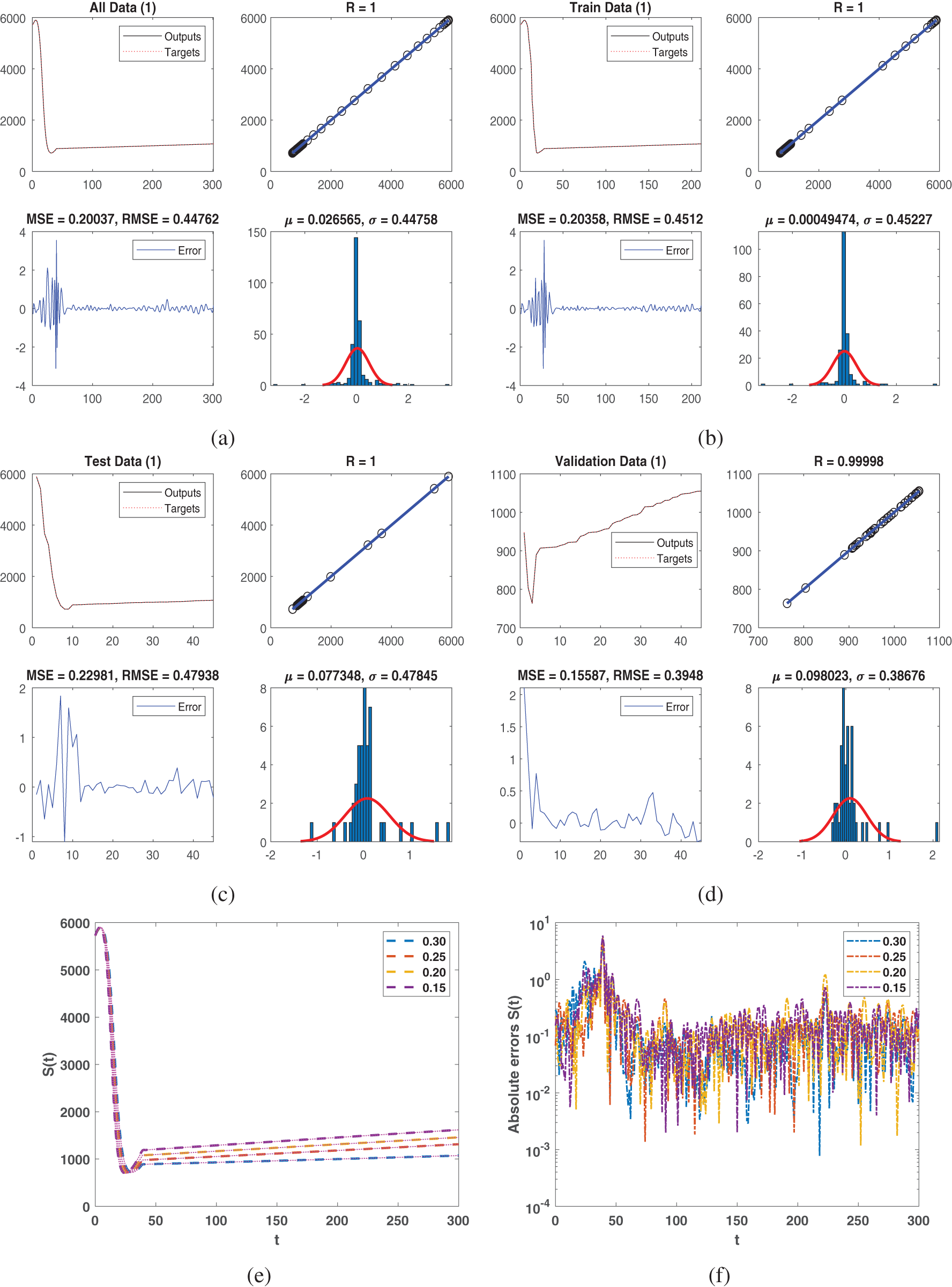
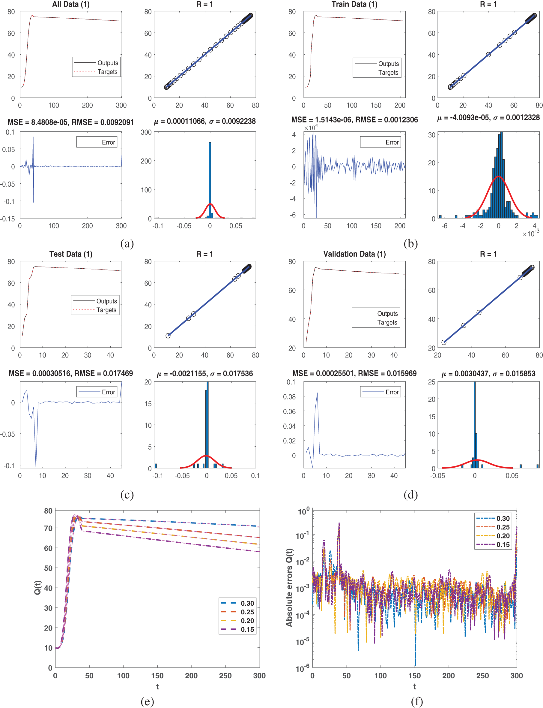
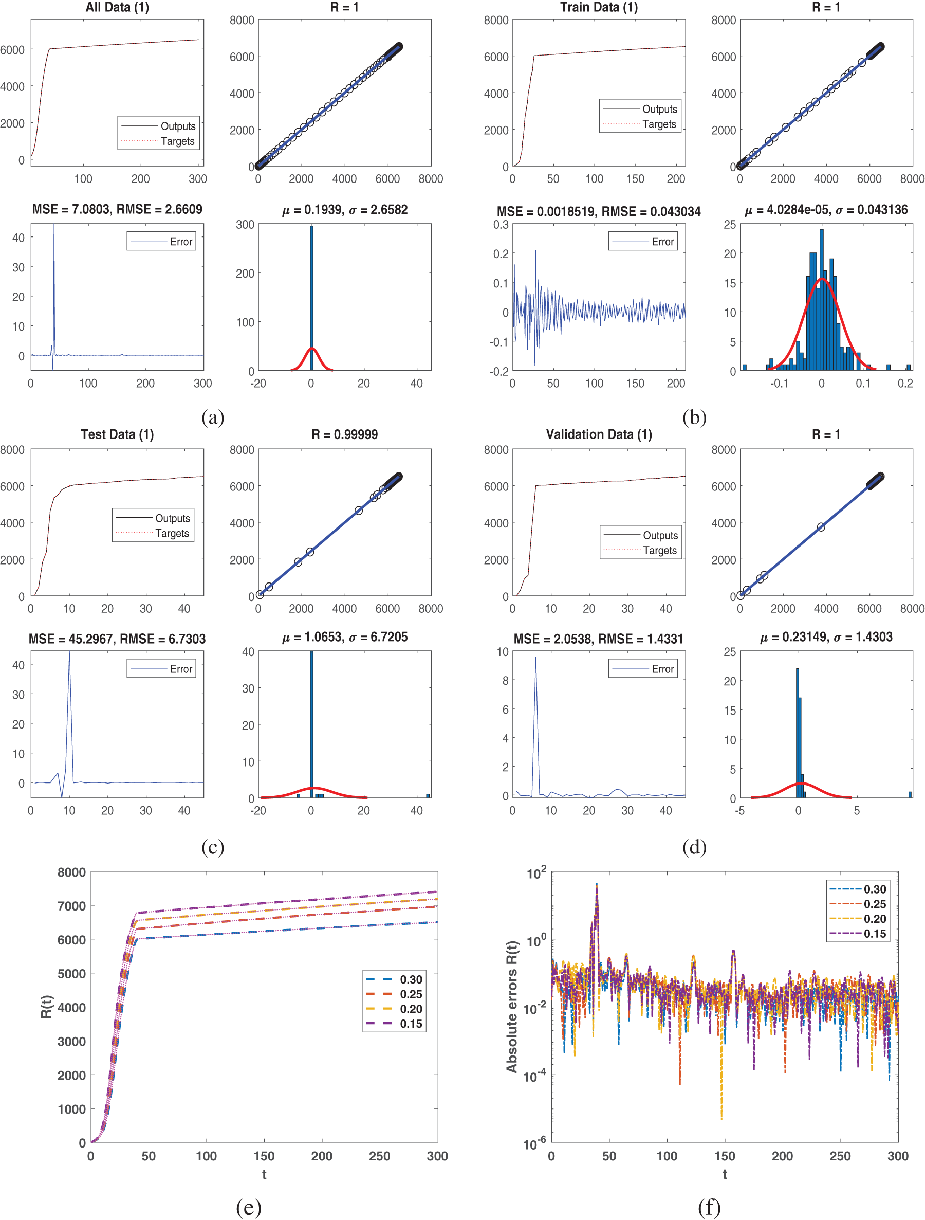
Our numerical simulation in Figs. 1 to 5, which uses the classical and global piece-wise AB derivative notion, is provided for the validation of the numerical method in this part. After splitting the interval into two sub-intervals, we verify that the first interval has an integer order derivative and compare it to Table 1’s available data for testing the second interval on various fractional orders in the sense of AB.
images

Figure 1: Piece-wise dynamical view of S(t) for factional order ψ in the first interval [0,t1] and second interval [t1,T] with NN (a) all points, (b) train points, (c) test points (d) validation (e) comparison plot (f) absolute error
images

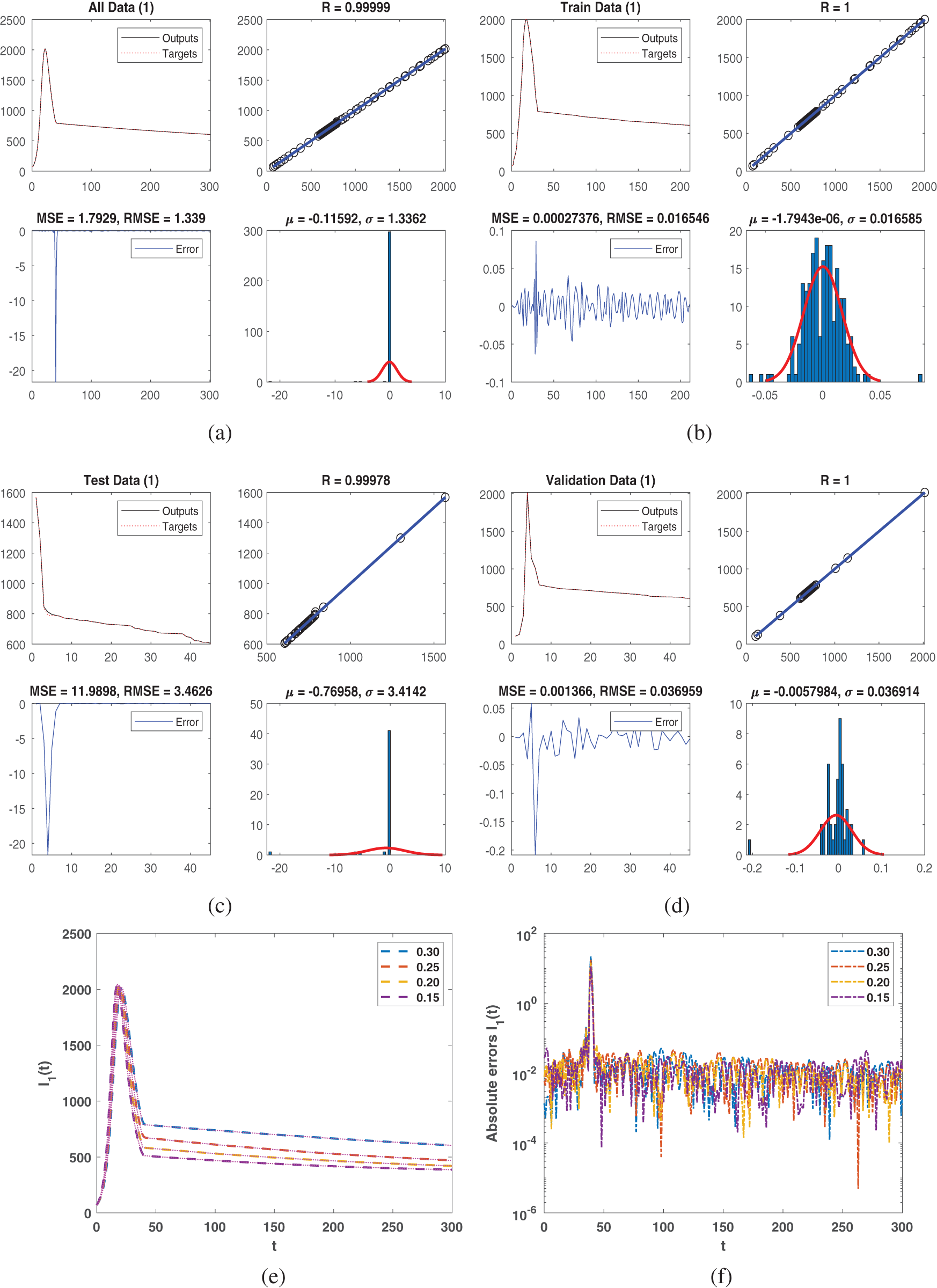
Figure 2: Piece-wise dynamical view of I1(t) for factional order ψ in the first interval [0,t1] and second interval [t1,T] with NN (a) all points, (b) train points, (c) test points (d) validation (e) comparison plot (f) absolute error
images

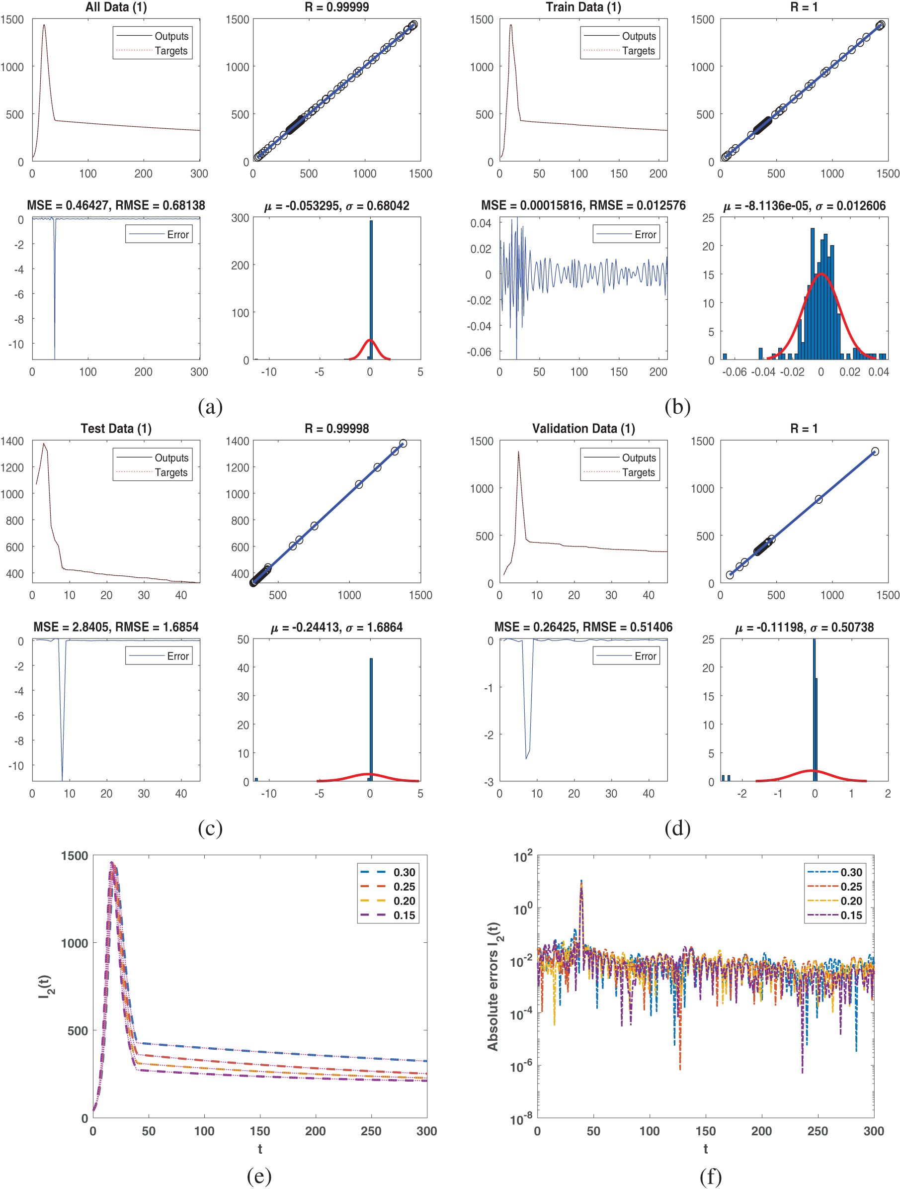
Figure 3: Piece-wise dynamical view of I2(t) for factional order ψ in the first interval [0,t1] and second interval [t1,T] with NN (a) all points, (b) train points, (c) test points (d) validation (e) comparison plot (f) absolute error
images

Figure 4: Piece-wise dynamical view of Q(t) for factional order ψ in the first interval [0,t1] and second interval [t1,T] with NN (a) all points, (b) train points, (c) test points (d) validation (e) comparison plot (f) absolute error
images

Figure 5: Piece-wise dynamical view of R(t) for factional order ψ in the first interval [0,t1] and second interval [t1,T] with NN (a) all points, (b) train points, (c) test points (d) validation (e) comparison plot (f) absolute error

Figs. 15 represent five agent populations in which the susceptible case decreases and then becomes stable as the other compartment increases on sub-intervals with bending from integer to fractional order. From [0,t1], the single curve line represents the integer order classical behavior for the first interval. Conversely, the global order derivative behavior on [t1,t2] is displayed by the four distinct curves for the second interval. In Fig. 2 the first stage infection of HIV slowly grows up in the first intervals and reaches its peak value it again declines moving towards stability in the second interval as the hospitalized and recovered people increase. Fig. 3 shows the dynamics of second-stage infection which behaves like 2 but with more time taken.

We address the piecewise Atangana-Baleanu-Caputo method with the NN approach for the previously mentioned model in this part. In this approach, we choose three types of hidden layers, including 10, 100, and 10 neurons for every layer to proceed the method onwards. Here, we applied the NN technique to obtain the performance of weight with low residual errors, and the epochs number is considered 1000. The obtained figures represented the approximate solution along with absolute error which we tested with NN to train the data accurately.

All data represented in Fig. 1a for class S and we obtained the output by using NN. Regression is 1 in this figure, and mean square (MS) and root mean square (RMS) errors are 0.20037 and 0.44762. To mention the method’s accuracy, the histogram shows a mean error of 0.026565 and a variance error of 0.44758. The train data in Fig. 1b for the same class produced the same output. Regression is one from Fig. 1b, while the MS and RMS errors are 0.20358 and 0.4512. As mentioned above, plot the mean error of 0.00049474 and the variance error of 0.45227 in the histogram. The test data we presented is in Fig. 1c, and the output is obtained with NN. The regression coefficient is approximately 1, while the mean and root mean square errors are 0.22981 and 0.47938, respectively. The histogram plot shows the mean error of 0.77348 and the variance error of 0.47845, and one can see the method’s accuracy. The validation data are plotted in Fig. 1d, and the results we obtained through NN show regression is approximately 1 while MS and RMS errors are 0.15587 and 0.3948, respectively. The histogram plot presents the mean error of 0.098023 and the variance error of 0.38676 to present the performance of the given approach. The dynamical behavior of S is shown as modified piecewise fractional along with NN in terms of Fig. 1e. The plot for absolute errors is represented as Fig. 1f.

All data represented in Fig. 2a for class I1 and we obtained the output with NN. This figure shows a regression coefficient of approximately 1. The MS and RMS errors are 1.7929 and 1.339, respectively. According to the histogram, the method has a mean error of 0.11592 and a variance error of 1.3362. The train data are in Fig. 2b and the results are obtained through NN. Fig shows the regression 1, MS, and RMS errors are 0.00027376 and 0.016546, respectively. Plot the mean error of 1.7943e06 and the variance error of 0.016585 on the histogram. The test data we presented is in Fig. 2c, and the results were obtained with the help of the NN approach. As a result, the regression is 1, while the MS and RMS errors are 11.9898 and 3.4626, respectively. This histogram plot shows a mean error of 0.76958 and a variance error of 3.4142, demonstrating the method’s accuracy. Validation data are plotted in Fig. 2d, and results are analyzed through NN, the regression is 1. 0.001366 is the MS, and 0.036959 is the RMS errors. To demonstrate the accuracy of the given technique, the histogram plot presents a mean error of 0.0057984 and a variance error of 0.0369614. A modified piecewise fractional model and an NN are shown for the first class as a function of Fig. 2e. Fig. 2f represents the plot for absolute errors.

All data are used NN to obtain the class I2 Fig. 3a output. This figure has an approximate regression coefficient of 1. The mean and root mean square errors are 0.46427 and 0.68138, respectively. The histogram shows a mean error of 0.053295 and a variance error of 0.68042. Fig. 3b shows the same output for train data with the same method for the same class. Based on the regression coefficient, the mean and root mean square errors are 0.0015816 and 0.012576, respectively, graph 8.1136e05 and the variance error of 0.012606 on the histogram. Similarly, the next figure shows the test data we presented. NN is used to obtain the output of Fig. 3c. Therefore, the regression coefficient of 2.8405, and the root mean square error of 1.6854. However, the mean error is 2.8405, while the root mean square error is 1.6854. According to this histogram plot, the method has a variance error of 1.6864 and a mean error of 0.24413. Validation data are plotted in Fig. 3d. The regression coefficient we obtained from NN is approximately one based on the output we obtained. There is a mean of 0.26425 and a root mean square error of 0.51406. Using the histogram plot, the mean and variance errors are 0.11198 and 0.50738, respectively, demonstrating the performance of the method. For the first class as a function of Fig. 3e, we show a modified piecewise fractional model and an NN Fig. 3f. A plot of absolute errors can be seen in Fig. 3f.

All data are represented in Fig. 4a. NN was used to obtain the output for class Q. Approximately 1 is the regression coefficient in this figure. Having calculated the mean and root mean square errors, we have found that the errors are 8.4808e05 and 0.0092091. To illustrate the method’s accuracy, the histogram indicates a mean error of 0.00011066 and a variance error of 0.0092238. The train data in Fig. 4 based on the same method, Fig. 4b also produced the same results for the same class. There is one regression coefficient in Fig. 4, while the mean and root mean square errors are 013.5143e06 and 0.0012306, respectively. Plot the mean error of 4.0093e05 and the variance error of 0.0012328 in the histogram. The test data we presented is in Fig. 4c, and results are obtained through NN. In this, regression is 1, while the mean and root mean square errors are 0.00030516 and 0.017459, respectively. One can see the method’s accuracy from the histogram plot, which shows a mean error of 0.0021155 and a variance error of 0.017536. The validation data are plotted in Fig. 4d. We obtained a regression coefficient of approximately 1 using NN. 0.00025501 and 0.015969 are the mean and root mean square errors, respectively. To demonstrate the accuracy of the technique, a histogram plot depicts the mean error of 0.0030437 and the variance error of 0.015853. Based on Fig. 4e, the dynamics of the first class are shown as modified piecewise fractional in conjunction with NN. As shown in the figure below, absolute errors are represented in Fig. 4f.

Fig. 5a represents all data. For class R, NN was used to obtain the output. Approximately 1 is the regression coefficient in this figure. Using the mean and root mean square errors, we found the errors to be 7.0803 and 2.6609. This histogram illustrates the method’s accuracy by showing a mean error of 0.1939 and a variance error of 2.6582. The train data in Fig. 5b and a similar method were used to produce the same results for the same class. According to Fig. 5b, one regression coefficient translates into a mean of 0.0018519 and a root mean square error of 0.043034, respectively. Plot the mean error of 4.0284e05 and the variance error of 0.043136 in the histogram. The test data we presented is in Fig. 5c, using NN, we obtain the output. This regression has an approximate 1 regression coefficient, a 45.2967 mean, and a 6.7303 root mean square error. The histogram plot demonstrates the method’s accuracy, with a mean error of 1.0653 and a variance error of 6.7205. The validation data are plotted in Fig. 5d. The regression coefficient obtained was approximately 1. In other words, 2.0538 is the mean error, and 1.4331 is the root mean square error. This histogram plot displays the mean error and variance error of 0.23149 and 1.4303, respectively, as a demonstration of the accuracy of the technique. A modified piecewise fractional in conjunction with a NN is shown in Fig. 5e. Here, absolute errors are shown as Fig. 5f.

6  Conclusion

The study analyzes a novel scheme of piece-wise derivable HIV infection with two two-stage infection models under the integer order derivative and AB operator, respectively. The considered system is treated on two sub-intervals by splitting the whole interval to establish the piece-wise dynamical system. The first interval is analyzed under integer order, while the second interval is processed under the global operator of AB derivative on different fractional orders. The uniqueness and existence in the form of theoretical results of both the intervals for the proposed model are proved using the analysis of fixed point theory. The numerical solution scheme for the model is also developed using Newton’s polynomial method for both sub-interval in integer order derivative and AB operator of fractional order ψ. The graphical view of all five agents has been shown for five different data on different arbitrary orders of the time interval. The bending effects are also shown on t1 describing crossover properties of the piece-wise derivative dynamics. The study analyzes a novel scheme of piece-wise derivable HIV infection with two two-stage infection models under the integer order derivative and AB operator, respectively. The considered system is treated on two sub-intervals by splitting the whole interval to establish the piece-wise dynamical system. The first interval is analyzed under integer order, while the second interval is processed under the global operator of AB derivative on different fractional orders. The uniqueness and existence in the form of theoretical results of both the intervals for the proposed model are proved using the analysis of fixed point theory.

Acknowledgement: We are thankful to the Deanship of Scientific Research at Imam Mohammad Ibn Saud Islamic University (IMSIU) (grant number IMSIU-RP23066).

Funding Statement: This work was supported and funded by the Deanship of Scientific Research at Imam Mohammad Ibn Saud Islamic University (IMSIU) (grant number IMSIU-RP23066).

Author Contributions: Ghaliah Alhamzi: Methodology, Writing—original draft, Formal analysis, Badr Saad T. Alkahtani: Conceptualization, Validation, Software, Ravi Shanker Dubey: Formal analysis, Validation, Software. Mati ur Rahman: Conceptualization, Supervision, Writing—original draft. All authors reviewed the results and approved the final version of the manuscript.

Availability of Data and Materials: All data generated or analyzed during this study are included in this published article.

Ethics Approval: Not applicable.

Conflicts of Interest: The authors declare no conflicts of interest to report regarding the present study.

References

1. Sakkoum A, Lhous M, Magri EM. A mathematical simulation and optimal control of a VIH model with different infectious level. J Math Comput Sci. 2022;12:117. [Google Scholar]

2. Anderson RM. The role of mathematical models in the study of HIV transmission and the epidemiology of AIDS. J Acquired Immune Def Synd. 1988;1(3):241–56. [Google Scholar] [PubMed]

3. Huo HF, Chen R, Wang XY. Modelling and stability of HIV/AIDS epidemic model with treatment. Appl Math Model. 2016;40(13–14):6550–9. doi:10.1016/j.apm.2016.01.054. [Google Scholar] [CrossRef]

4. Granich RM, Gilks CF, Dye C, De Cock KM, Williams BG. Universal voluntary HIV testing with immediate antiretroviral therapy as a strategy for elimination of HIV transmission: a mathematical model. Lancet. 2009;373(9657):48–57. doi:10.1016/S0140-6736(08)61697-9. [Google Scholar] [PubMed] [CrossRef]

5. Li Z, Teng Z, Miao H. Modeling and control for HIV/AIDS transmission in China based on data from 2004 to 2016. Comput Math Methods Med. 2017;2017(1):8935314. doi:10.1155/2017/8935314. [Google Scholar] [PubMed] [CrossRef]

6. May RM, Anderson RM. Commentary transmission dynamics of HIV infection. Nature. 1987;326:137–42. [Google Scholar] [PubMed]

7. Ngina P, Mbogo RW, Luboobi LS. Modelling optimal control of in-host HIV dynamics using different control strategies. Comput Math Methods Med. 2018;2018(1):9385080. doi:10.1155/2018/9385080. [Google Scholar] [PubMed] [CrossRef]

8. Singh R, Ali S, Jain M, Rakhee. Epidemic model of HIV/AIDS transmission dynamics with different latent stages based on treatment. Am J Appl Mathemat. 2016;13(2):222–34. doi:10.11648/j.ajam.20160405.14. [Google Scholar] [CrossRef]

9. Shen M, Xiao Y, Rong L. Global stability of an infection-age structured HIV-1 model linking within-host and between-host dynamics. Mathemat Biosci. 2015;263:37–50. doi:10.1016/j.mbs.2015.02.003. [Google Scholar] [PubMed] [CrossRef]

10. Shi S, Nguyen PK, Cabral HJ, Diez-Barroso R, Derry PJ, Kanahara SM, et al. Development of peptide inhibitors of HIV transmission. Bioact Mater. 2016;1(2):109–21. doi:10.1016/j.bioactmat.2016.09.004. [Google Scholar] [PubMed] [CrossRef]

11. Shirazian M, Farahi MH. Optimal control strategy for a fully determined HIV model. Intell Control Automat. 2010;1(1):15–9. doi:10.4236/ica.2010.11002. [Google Scholar] [CrossRef]

12. Silva CJ, Torres DF. Modeling and optimal control of HIV/AIDS prevention through PrEP. Discrete Contin Dyn Syst Ser S. 2017;11:119–41. [Google Scholar]

13. Umar M, Sabir Z, Amin F, Guirao JLG, Raja MAZ. Stochastic numerical technique for solving HIV infection model of CD4+ T cells. Eur Phys J Plus. 2020;135(5):403. doi:10.1140/epjp/s13360-020-00417-5. [Google Scholar] [CrossRef]

14. Işık E, Daşbaşı B. A compartmental fractional-order mobbing model and the determination of its parameters. Bull Biomathemat. 2023;1(2):153–76. doi:10.59292/bulletinbiomath.2023008. [Google Scholar] [CrossRef]

15. Bolaji B, Onoja T, Agbata C, Omede BI, Odionyenma UB. Dynamical analysis of HIV-TB co-infection transmission model in the presence of treatment for TB. Bull Biomathemat. 2024;2(1):21–56. doi:10.59292/bulletinbiomath.2024002. [Google Scholar] [CrossRef]

16. Kumar P, Erturk VS. Dynamics of cholera disease by using two recent fractional numerical methods. Mathemat Modell Numer Simulat Appl. 2021;1(2):102–11. doi:10.53391/mmnsa.2021.01.010. [Google Scholar] [CrossRef]

17. Ahmed I, Akgül A, Jarad F, Kumam P, Nonlaopon K. A Caputo-Fabrizio fractional-order cholera model and its sensitivity analysis. Mathemat Modell Numer Simulat Appl. 2023;3(2):170–87. doi:10.53391/mmnsa.1293162. [Google Scholar] [CrossRef]

18. Atangana A, Baleanu D. New fractional derivatives with nonlocal and non-singular kernel: theory and application to heat transfer model. J Thermal Sci. 2016;20(2):763–9. doi:10.2298/TSCI160111018A. [Google Scholar] [CrossRef]

19. Fatima B, Yavuz M, Rahman MU, Al-Duais FS. Modeling the epidemic trend of middle eastern respiratory syndrome coronavirus with optimal control. Math Biosci Eng. 2023;20(7):11847–74. doi:10.3934/mbe.2023527. [Google Scholar] [PubMed] [CrossRef]

20. Mahmood T, ur Rahman M, Arfan M, Kayani SI, Sun M. Mathematical study of Algae as a bio-fertilizer using fractal–fractional dynamic model. Mathemat Comput Simulat. 2023;203(2):207–22. doi:10.1016/j.matcom.2022.06.028. [Google Scholar] [CrossRef]

21. Mahmood T, Al-Duais FS, Sun M. Dynamics of Middle East respiratory syndrome coronavirus (MERS-CoV) involving fractional derivative with Mittag-Leffler kernel. Phys A: Statis Mech Appl. 2022;606(26):128144. doi:10.1016/j.physa.2022.128144. [Google Scholar] [PubMed] [CrossRef]

22. Atangana A, Araz Sİ. Nonlinear equations with global differential and integral operators: existence, uniqueness with application to epidemiology. Results Phys. 2021;20(2):103593. doi:10.1016/j.rinp.2020.103593. [Google Scholar] [CrossRef]

23. Haidong Q, ur Rahman M, Arfan M, Salimi M, Salahshour S, Ahmadian A. Fractal–fractional dynamical system of Typhoid disease including protection from infection. Eng Comput. 2023;39:1553–1562. [Google Scholar]

24. Mahmood T, Al-Duais FS, Sami A, Sun M. Analysis of tritrophic interaction with volatile compounds in plants with fractal fractional caputo operator. Fractals. 2023;31(10):2340082. doi:10.1142/S0218348X23400820. [Google Scholar] [CrossRef]

25. Awadalla M, Mu R, Al-Duais FS, Al-Bossly A, Abuasbeh K, Arab M. Exploring the role of fractal-fractional operators in mathematical modelling of corruption. Appl Mathemat Sci Eng. 2023;31(1):2233678. doi:10.1080/27690911.2023.2233678. [Google Scholar] [CrossRef]

26. Li B, Zhang T, Zhang C. Investigation of financial bubble mathematical model under fractal-fractional Caputo derivative. Fractals. 2023;31(5):14. doi:10.1142/S0218348X23500500. [Google Scholar] [CrossRef]

27. Baleanu D, Ghassabzade FA, Nieto JJ, Jajarmi A. On a new and generalized fractional model for a real cholera outbreak. Alexandria Eng J. 2022;61(11):9175–86. [Google Scholar]

28. Li B, Eskandari Z. Dynamical analysis of a discrete-time SIR epidemic model. J Frankl Inst. 2023;360(12):7989–8007. [Google Scholar]

29. Iwa LL, Nwajeri UK, Atede AO, Panle AB, Egeonu KU. Malaria and cholera co-dynamic model analysis furnished with fractional-order differential equations. Mathemat Modell Numer Simul Appl. 2023;3(1):33–57. [Google Scholar]

30. Atangana A, İğret Araz S. Mathematical model of COVID-19 spread in Turkey and South Africa: theory, methods, and applications. Adv Diff Equat. 2020;2020:1–89. [Google Scholar]

31. Atangana A, Araz Sİ. New concept in calculus: piecewise differential and integral operators. Chaos, Solit Fract. 2021;145:110638. [Google Scholar]


Cite This Article

APA Style
Alhamzi, G., Alkahtani, B.S.T., Dubey, R.S., ur Rahman, M. (2025). Global piecewise analysis of HIV model with bi-infectious categories under ordinary derivative and non-singular operator with neural network approach. Computer Modeling in Engineering & Sciences, 142(1), 609-633. https://doi.org/10.32604/cmes.2024.056604
Vancouver Style
Alhamzi G, Alkahtani BST, Dubey RS, ur Rahman M. Global piecewise analysis of HIV model with bi-infectious categories under ordinary derivative and non-singular operator with neural network approach. Comput Model Eng Sci. 2025;142(1):609-633 https://doi.org/10.32604/cmes.2024.056604
IEEE Style
G. Alhamzi, B. S. T. Alkahtani, R. S. Dubey, and M. ur Rahman, “Global Piecewise Analysis of HIV Model with Bi-Infectious Categories under Ordinary Derivative and Non-Singular Operator with Neural Network Approach,” Comput. Model. Eng. Sci., vol. 142, no. 1, pp. 609-633, 2025. https://doi.org/10.32604/cmes.2024.056604


cc Copyright © 2025 The Author(s). Published by Tech Science Press.
This work is licensed under a Creative Commons Attribution 4.0 International License , which permits unrestricted use, distribution, and reproduction in any medium, provided the original work is properly cited.
  • 77

    View

  • 20

    Download

  • 0

    Like

Share Link