Landslide Susceptibility Mapping Using RBFN-Based Ensemble Machine Learning Models

1  Introduction

Landslides are a significant natural hazard, causing substantial loss of life and property in the affected areas. The United Nations Office for Disaster Risk Reduction (UNDRR) reports that landslides are responsible for an average of 25,000 deaths per year globally [1]. The majority of these deaths occur in developing countries, where infrastructure and emergency response systems may be less developed. In addition to the loss of life, landslides also cause significant economic and social disruption, leaving many people homeless and destroying livelihoods, leading to long-term consequences. Data from the Centre for Research on the Epidemiology of Disasters (CRED) shows that during 2000–2019, disaster types that includes landslides were responsible for 42,564 deaths, approximately 3% of total deaths from natural hazards over this period [2].

Mapping areas susceptible to landslides is a primary step in managing and reducing landslide-related damages through proper land use planning and decision making [3]. Landslide susceptibility mapping identifies areas likely to experience landslide occurrences in the future. To obtain accurate and reliable maps of landslide susceptibilities, Machine Learning (ML) based models are recognized as better quantitative techniques than traditional weighted methods and expert opinion-based techniques [4]. These models use algorithms and statistical techniques to analyze spatial relationship between landslide-affecting factors and historical landslide occurrences in a certain area, allowing for the prediction of landslide likelihood in new or unobserved areas. Many ML-based models, such as Random Forest (RF) [5], Support Vector Machines (SVM) [6], Support Vector Regression (SVR) [7], Artificial Neural Networks (ANN) [8], Decision Trees [9], Adaptive Neuro-Fuzzy Inference System (ANFIS) [10], and Group Method of Data Handling (GMDH) [11] have been effectively applied in various landslide-prone areas worldwide. These ML models have generally shown superior and promising results in landslide susceptibility mapping.

Over the past years, advanced ML models have been developed and applied for landslide susceptibility mapping, including various ensemble models [12]. Ensemble models combine multiple individual models or classifiers to generate more reliable and accurate predictions of landslide susceptibility. In literature, Di Napoli et al. [13] presented a novel approach which was the ensemble of generalized boosting, ANN, and maximum entropy for mapping landslide susceptibility in the Monterosso al Mare area, Italy, and stated that the novel ensemble approach received an improved reliability compared with single models. Hong et al. [14] developed two novel ensemble ML namely LADT-Bagging and FPA-Bagging which were combinations of Bagging and two single classifiers such as LogitBoost alternating decision trees (LADT) and Forest by Penalizing Attributes (FPA), and stated that the developed ensemble models are promising tools for modeling landslide susceptibility in the Youfanggou district (China). Pham et al. [15] integrated Reduced Error Pruning Tree (REPT) with the Bagging, Decorate, and Random Subspace ensemble learning techniques for predicting rainfall-induced landslides in the Uttarkashi district of India. Lv et al. [16] assessed landslide susceptibility mapping using four Heterogeneous Ensemble Learning (HEL) models with different ML models such as Convolutional Neural Network (CNN), Deep Belief Network (DBN), and deep Residual Network (ResNet) at the Three Gorges Reservoir area, China, and stated that the HEL-based models showed better stability compared with single ML models as they can avoid the overfitting problems. Bien et al. [17] developed and compared four ensemble models which were combinations of three optimization techniques such as Bagging, Decorate, and Random Subspace and a single classifier namely Fuzzy Unordered Rules Induction Algorithm (FURIA) for landslide susceptibility mapping at Lai Chau Province (Vietnam), and stated that these four proposed models are better than single models such as FURIA and SVM. Teke et al. [9] employed the J48 decision tree in conjunction with AdaBoost, Bagging, and Rotation Forest methods to classify landslide susceptibility in China. Saha et al. [18] combined RF with Bagging, Rotation Forest, and Random Subspace techniques. Tran et al. [19] utilized the Hyperpipes algorithm to develop five novel ensemble models that integrate the Hyperpipes algorithm with various ensemble techniques, including AdaBoost, Bagging, Dagging, Decorate, and Real AdaBoost for mapping the spatial variability of landslide susceptibility in Ha Giang Province, Vietnam. Pham et al. [20] developed three ensemble predictive models aimed at predicting landslide susceptibility in the Dien Bien Province, Vietnam, combining Multiclass Alternating Decision Trees method with Dagging, MultiboostAB, and Random Subspace ensemble learning techniques. Hong [21] merged the Best First Decision Tree with Bagging, Cascade generalization, Decorate, MultiboostAB, and Random SubSpace for landslide susceptibility mapping. Le Minh et al. [22] combined Dagging, Bagging, and Decorate ensemble techniques with a Radial Basis Function Network (RBFN) to predict landslide susceptibility in the Cao Bang Province, Vietnam. In general, the studies mentioned demonstrate the significant potential of ensemble ML models to enhance the effectiveness of landslide susceptibility assessments, while also indicating room for further improvement [23–26].

In this study, our primary goal is to enhance the performance of landslide susceptibility modeling by developing innovative ensemble ML models. These models, known as DG-RBFN, MB-RBFN, and AB-RBFN, combine RBFN with various ensemble techniques such as DAGGING, MULTIBOOST, and ADABOOST. By utilizing these novel approaches, we aim to improve the accuracy and reliability of landslide predictions. The key novelty of this study lies in developing and applying these ensemble models for assessing landslide susceptibility in the Pithoragarh area of Uttarakhand, India. This is the first time these ensemble models have been employed for this purpose. The models were validated and compared using several standard metrics, including the area under the ROC curve. Additionally, a traditional weighted method, the Information Value (IV) Model, and a benchmark ML model, the Multilayer Perceptron Neural Network (MLP), were used for comparison and validation. Weka and ArcGIS were utilized for modeling and mapping in this study.

2  Material and Methods

2.1 Description of the Study Area

The study area is located in the Pithoragarh district of Uttarakhand, India, which regularly experiences landslides of varying scales. The study area is situated between latitudes 29°30′00″N to 30°00′00″N and longitudes 80°00′00″E to 80°30′00″E (Fig. 1). The Pithoragarh district is a hilly terrain region with several high peaks reaching heights up to approximately 4200 m. In the northeast region, slopes and cliffs are ranging from high to moderate altitudes. The southeast area consists of moderately dissected rugged hills with a number of low terraces and high slopes at the foot of the mountains. The northwest part features hills characterized by valley walls from high to average slopes along the tributary Goriganga River. The southeast corner of the study area is laden with thick alluvium brought by the Rauntis Gad River, mixed with hillslope processes and transported debris. There are several tectonic structures, some active and some dormant, passing through or around the area, including the Berinag thrust, Ramgarh thrust, Almora thrust, North Almora thrust (NAT), South Almora Thrust (SAT), and numerous other faults. The main drainage system in the Goriganga River basin is characterized by fluvial terraces, mostly along the right bank of the stream, while the left bank features steep valley walls for a considerable stretch of the channel. From south to north, the study area reveals the rocks of the Almora group and Garhwal groups. The Garhwal group rocks comprise granitoids embedded with Chipkot and Askot group rocks. Shale, slate, phyllite (a variation of shale), quartz, dolomite (a carbonate sedimentary rock), limestone, magnesite, calcareous stone, and metavolcanics (rocks created by volcanic activity) are found in the Garhwal group. Pithoragarh district experiences a wide range of temperature variations due to altitudinal differences. Temperatures rise from mid-March to mid-June. High-altitude areas above approximately 3500 m (11,500 feet) always remain under permanent snow cover. In places like River Gorge Dharchula, Jhulaghat, Ghat, and Sera, temperatures can reach up to 40°C (104°F). The mean annual rainfall in the downstream area is 360 cm (140 inches). The information on the study area is referenced from the report of the Indian Geological Association (https://www.gsi.gov.in/webcenter/portal/ocbis/pagequicklinks/pageprojects) (accessed on 29 September 2024).

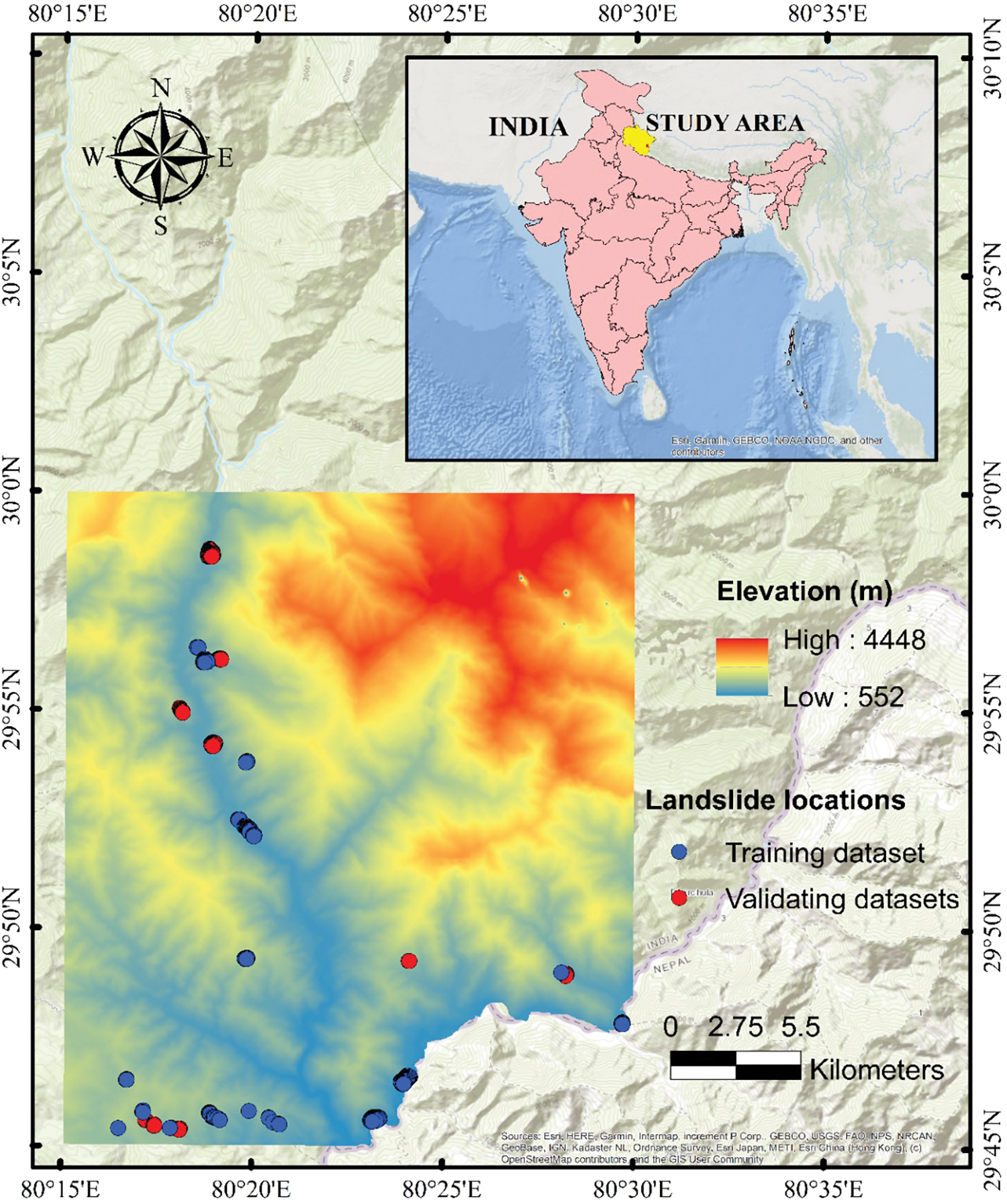
Figure 1: Location of the study area and historical landslides

2.2 Landslide Inventory

A landslide inventory was compiled based on an extensive analysis of Google Earth images [27], supplemented by data extracted from reference reports published by the Geological Survey of India (https://www.gsi.gov.in) (accessed on 29 September 2024). A total of 34 landslide events were identified and mapped in the study area (Figs. 1 and 2). Each of these landslide events was initially represented as a polygon, which outlines the affected area on a map. For the purposes of analysis, a conversion of these polygons into a different format was necessary. Therefore, the 34 landslide polygons were transformed into points, resulting in 261 individual points that are suitable for spatial analysis. This conversion was essential, as spatial modeling of landslides relies on point and raster data for its calculations. By transforming the polygons into points, the data became compatible with the software’s processing requirements, enabling a more accurate analysis of landslide susceptibility [28]. The data from this study was also utilized and presented in Ngo et al. [29].

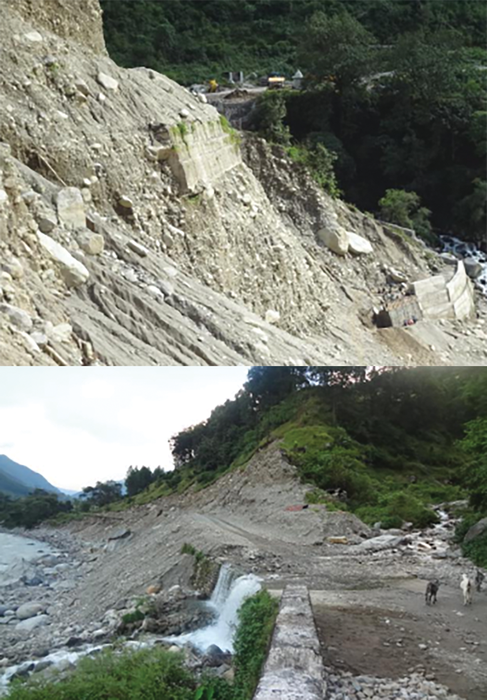
Figure 2: Photographs showing landslide occurrence in the study area (Source: http://www.portal.gsi.gov.in) (accessed on 29 September 2024)

The mass movement events included in this study are primarily of two types: rock landslides and debris slides. From the total inventoried landslide database, 70% of the data, along with corresponding values of landslide conditioning factors, was used for training the models, while 30% was reserved for validation.

2.3 Landslide Conditioning Factors

Selecting the factors that contribute to landslides is a crucial step in assessing landslide susceptibility. In this study, ten conditioning factors were chosen based on an analysis of past landslides, the geo-environmental characteristics of the study area, data availability, and a review of similar published works [7]. These factors include slope, aspect, curvature, elevation, land cover, lithology, geomorphology, distance to rivers, distance to roads, and overburden depth. The correlation analysis of the input variables is illustrated in Fig. 3. It is important to note that all conditioning factors obtained from the Geological Survey of India (GSI) report were resampled to a 30 m resolution to ensure homogeneity among them. A brief description of the conditioning factors included in the study is provided in the following paragraphs.

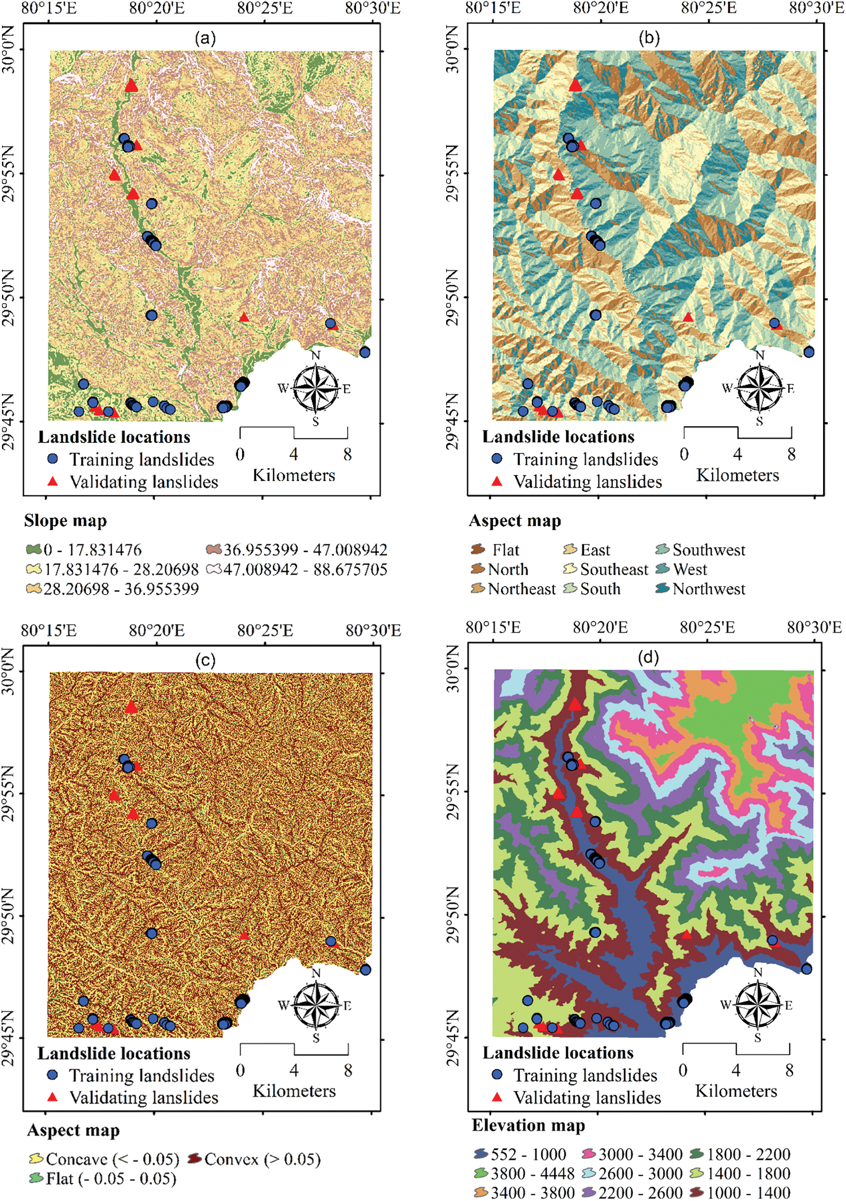
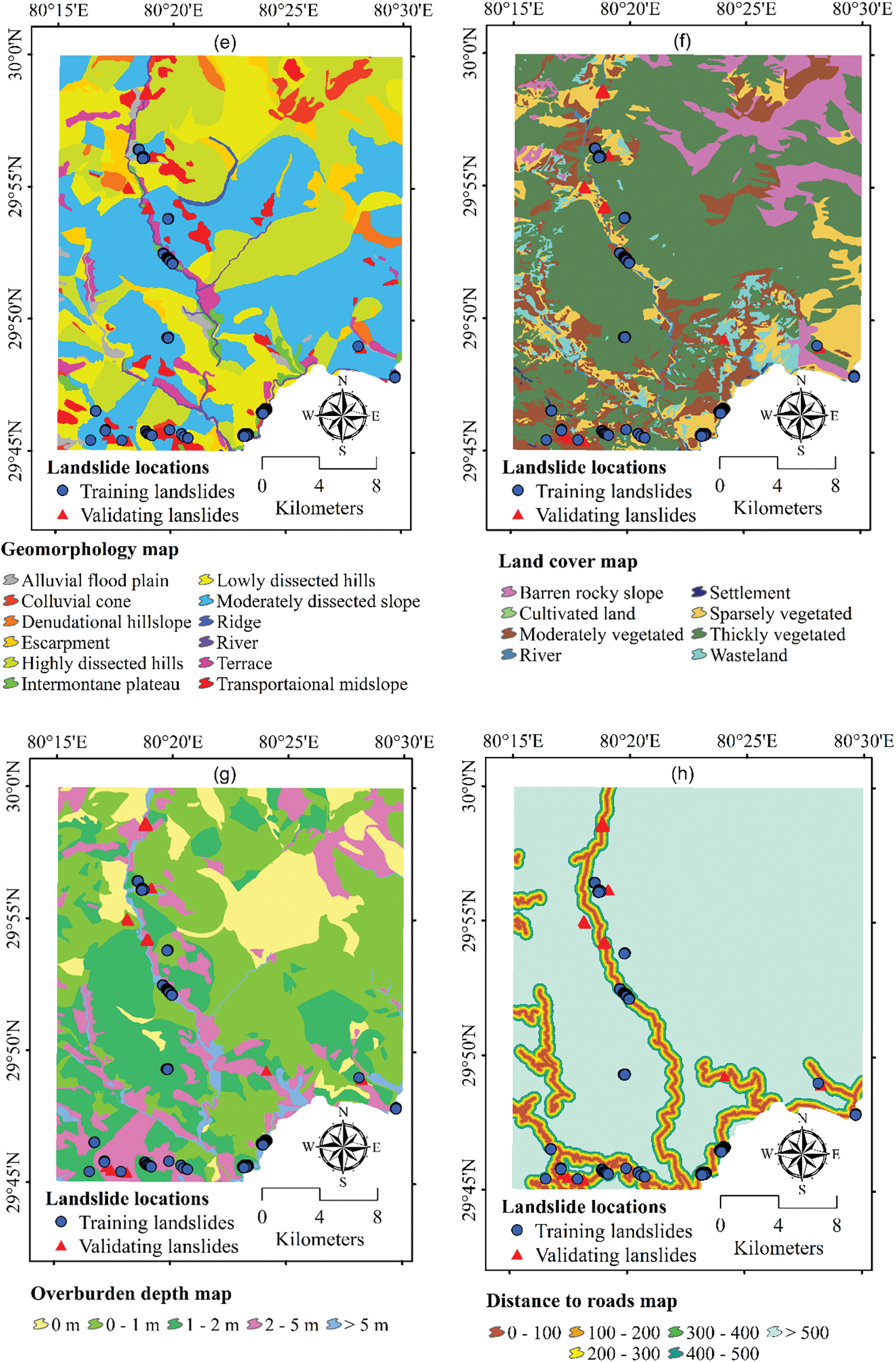
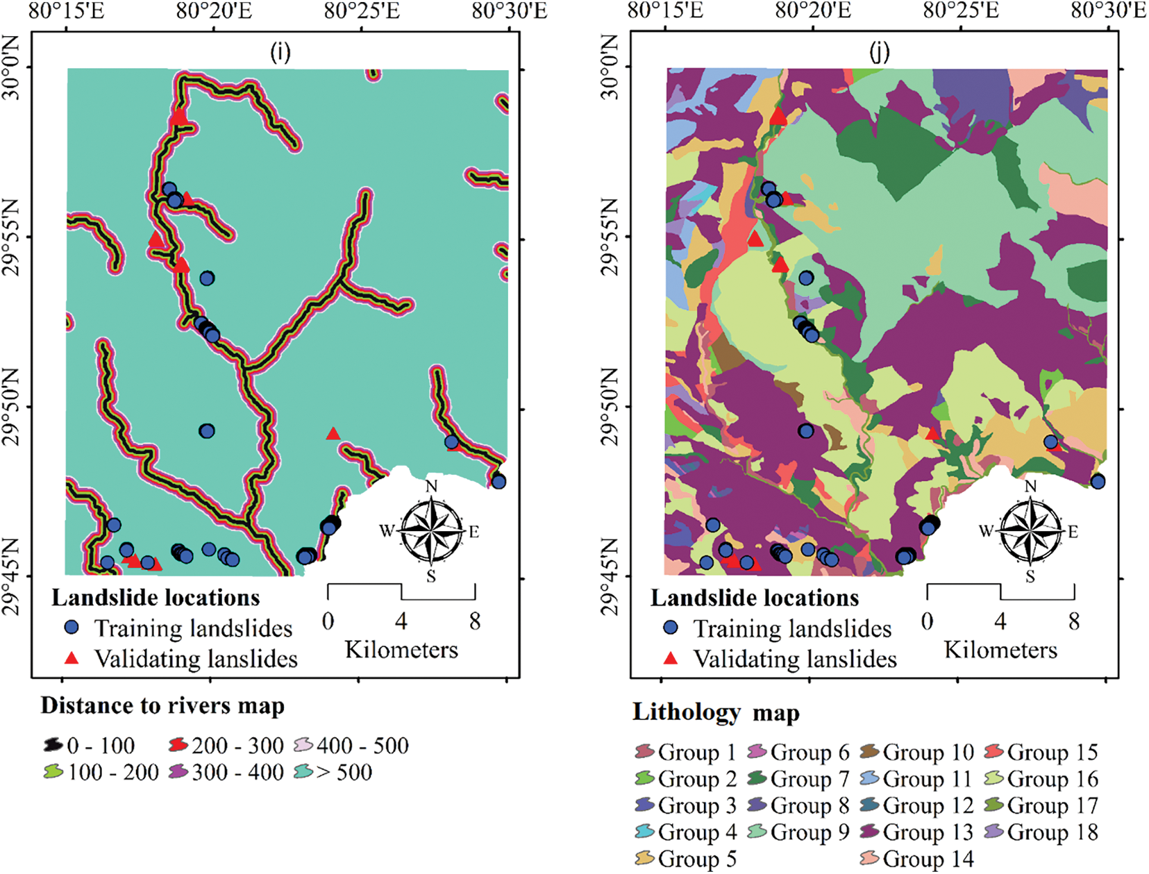
Figure 3: The map of the conditioning factors used in this study (a) slope, (b) aspect, (c) curvature, (d) elevation, (e) geomorphology, (f) land cover, (g) overburden depth, (h) distance to roads, (i) distance to rivers, and (j) lithology

Slope

Slope refers to the inclination or angle of a surface in relation to the horizontal plane. It measures the steepness of landforms such as hills, mountains, or valleys and can be expressed in terms of degree or gradient. The slope of a surface is determined by the relationship between its vertical height change and its horizontal distance along the surface. Slope is a critical factor in geomorphology and the analysis of geohazards, including landslides, erosion, and mass movements [30,31]. In this study, the slope angle map was derived from the ALOS PALSAR 30 m Digital Elevation Model (DEM) obtained from ALOS Data Collection [32,33]. The slope angle map was then reclassified into five classes using the Natural Breaks method within a GIS environment, as follows: 0–17.83°, 17.83–28.21°, 28.21–36.96°, 36.96–47.01°, and 47.01–88.68° (Fig. 3a).

Aspect

Aspect refers to the direction a slope faces on a geomorphic surface, typically categorized as north-facing, south-facing, east-facing, or west-facing. This directional orientation significantly impacts the amount and distribution of solar radiation, wind exposure, and temperature on the slope. Consequently, these factors play a crucial role in influencing vegetation growth, soil properties, and the processes of erosion and sediment transport. For instance, south-facing slopes may receive more sunlight, promoting different vegetation types compared to north-facing slopes, which tend to be cooler and moister [34]. In this study, a slope direction map was generated from the ALOS PALSAR 30 m DEM in a GIS environment. The aspect map was classified into nine categories as depicted in Fig. 3b.

Curvature

Curvature refers to the extent to which a surface deviates from being flat; and is expressed as the change in the slope of the surface over a given distance. In geomorphology, surface curvature is used to describe the shape of landforms such as hills and valleys; and can be quantified using mathematical techniques such as topographic profiles and digital elevation models. Surface curvature significantly influences the flow of water and air across the terrain, thereby affecting processes such as erosion, sediment deposition, and even landslide occurrences [35]. For instance, convex surfaces may promote faster runoff, while concave surfaces can collect water, leading to increased erosion in certain areas. In this study, the terrain surface shape map was derived from the DEM and classified into three categories: concave, convex, and flat (Fig. 3c).

Elevation

Elevation (also termed as altitude) in geomorphology refers to the height of a location or feature above a reference surface, typically sea level. Elevation can be used to describe the vertical position of landforms such as mountains, valleys, and plateaus, and is an important factor in determining local climate patterns, as well as the distribution of vegetation and other biotic factors [36,37]. Elevation data is commonly obtained through satellite imagery, laser-based systems, and other remote sensing techniques, which allow researchers to create detailed DEMs of the Earth’s surface [38,39]. To aid in understanding the spatial distribution of elevation-related factors in the study area, the terrain elevation map of the study area was generated from the DEM and classified into nine distinct elevation ranges: 552–1000 m, 1000–1400 m, 1400–1800 m, 1800–2200 m, 2200–2600 m, 2600–3000 m, 3000–3400 m, 3400–3800 m, and above 3800 m (Fig. 3d).

Geomorphology

Geomorphology plays a crucial role in landslide studies, as it helps explain the underlying causes and triggering mechanisms of these events. By analyzing factors such as slope angle, surface curvature, soil type, vegetation cover, and the presence of fractures or faults, geomorphology provides valuable insights into the conditions that can lead to landslides [40,41]. Additionally, it considers the effects of rainfall, earthquakes, and other triggers that may initiate a landslide. This information is essential for developing hazard assessments and informing mitigation and management strategies to reduce landslide risk and protect human and environmental assets [42,43]. In this study, the geomorphological map was obtained from the survey report of the Indian Geological Survey of India, which classifies the study area into 12 distinct geomorphic classes (Fig. 3e).

Land Use and Land Cover (LULC)

LULC is another important factor in landslide susceptibility modeling. LULC data provides information on vegetation cover, soil type, surface permeability, surface runoff, and topography [44,45], all of which can impact slope stability and increase the risk of landslides. The LULC data for the study area was collected from the survey report of the Indian Geological Survey of India (Fig. 3f).

Overburden depth

Overburden depth, or the thickness of the material covering the underlying rock or soil, also plays a significant role in slope stability and landslide likelihood. The added weight and reduced strength of the underlying material due to overburden can contribute to slope failure [46]. In this study, overburden depth data was collected from the Geological Survey of India web portal and reclassified into five classes as shown in Fig. 3g.

Distance to roads

The proximity of an area to roads can also influence slope stability and landslide risk. Roads, which indicate the presence of transportation infrastructure and human activity, can lead to soil erosion, changes in drainage patterns, and landscape alterations, all of which can contribute to slope instability [47]. In this study, the road network was digitized from satellite images extracted from Google Earth, and the distance to roads was classified into six classes as shown in Fig. 3h.

Distance to rivers

Distance to rivers is another important conditioning factor in landslide susceptibility modeling, as it affects groundwater levels and drainage patterns, which can impact slope stability [48,49]. In this study, the stream network extracted from the DEM was used to create the distance classes from the streams, which were then reclassified into six classes (Fig. 3i).

Lithology

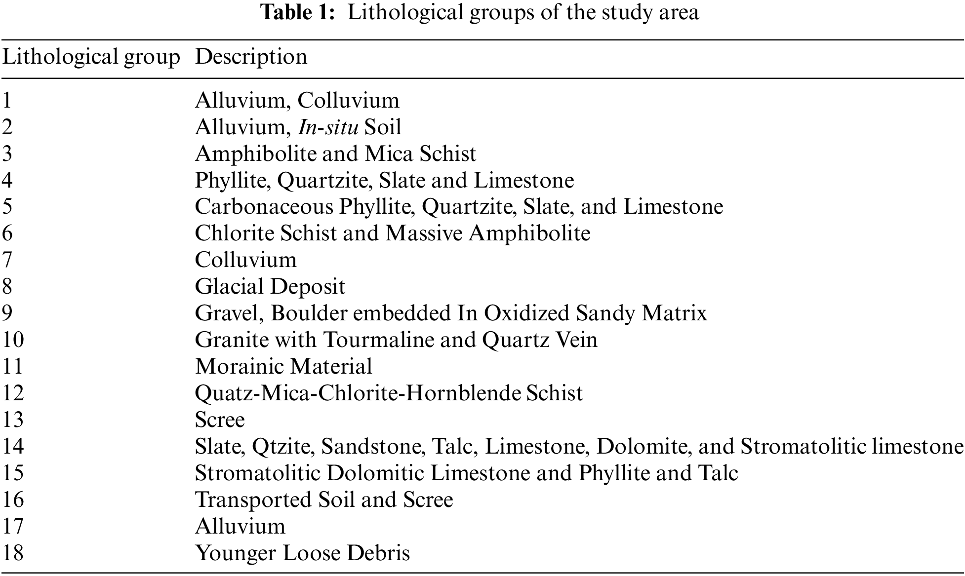
Lithology, or the materials forming slopes, directly affects landslide occurrence [50]. In this study, slope-based material maps were built using data collected from the Geological Survey of India. The types of materials forming slopes in the study area are presented in Ngo et al. [29] (Fig. 3j and Table 1).

2.4 Methods Used

2.4.1 Factor Evaluation Methods

Before utilizing the conditioning factors to assess landslide susceptibility, it is essential to evaluate them for their correlation and significance. This evaluation can be effectively conducted using the Pearson correlation method and the Information Gain Ratio method [12,51]. The primary objective of this process is to identify and eliminate highly correlated and unimportant factors, which can improve the overall performance and accuracy of the models. The Pearson correlation method helps determine the strength and direction of the linear relationship between pairs of conditioning factors. By analyzing these correlations, redundant factors that provide similar information and may lead to model overfitting or reduced interpretability can be identified. On the other hand, the Information Gain Ratio method assesses the importance of each conditioning factor in predicting landslide susceptibility. This method quantifies how much information a particular factor contributes to the prediction, allowing for the prioritization of factors that have the most significant impact on landslide occurrence. Information Gain Ratio method is particularly effective in handling high-dimensional datasets, where selecting a subset of relevant features can greatly simplify the model and improve computational efficiency. By reducing the dimensionality of the feature space, Information Gain Ratio method helps to alleviate the curse of dimensionality and mitigate the risk of overfitting. It allows the model to focus on the most discriminative features, which enhances its predictive accuracy and generalization ability. In this study, Information Gain Ratio method feature selection was select to evaluate and select the important landslide conditioning factors for landslide susceptibility modeling and mapping using ML models.

2.4.2 Information Value Model

Information Value (IV) method is a bivariate statistical technique used to calculate the relationship between landslide conditioning factors and the occurrence of landslides, which is treated as a binary target variable (landslide or no landslide) [52]. In this approach, information values are calculated for each class of the conditioning factor maps based on the presence of landslides in a given map unit. These information values help determine the role and contribution of each factor class to landslide occurrence [53].

To apply the IV method, all conditioning factors are first converted into raster format with the same coordinate system and pixel size (typically 30 m × 30 m), and then reclassified into different classes. The information value for a specific factor class is calculated using the logarithm of the ratio of conditional probability to prior probability, as follows [54]:

IV=log⁡(P(A)P(B))=log⁡(Nslpix/NcpixNtspix/Ntapix)(1)

where Nslpix is the number of landslide pixels in a certain layer, Ncpix is the number of pixels in a certain layer, Ntspix is the total number of landslides in the study area, and Ntapix is a total pixel in the entire study area.

The IV values calculated for each factor class represent the probability of landslide occurrence in that class relative to the overall landslide probability in the study area. If the IV value for a factor class is greater than 0.1, it indicates a positive correlation with landslide occurrence, meaning that class has a higher probability of landslides. Conversely, negative IV values suggest a lower probability of landslides for that factor class. By analyzing the IV values for different factor classes, researchers can identify the most influential conditioning factors and their specific classes that contribute significantly to landslide susceptibility. This information is crucial for developing accurate landslide susceptibility maps and implementing targeted mitigation strategies in landslide-prone areas. The IV method has been widely applied in various studies for landslide susceptibility mapping due to its ability to quantify the relationship between landslide conditioning factors and landslide occurrence using statistical principles. It provides a straightforward and effective way to assess the importance of different factors and their classes in predicting landslide susceptibility.

2.4.3 Radial Basis Function Networks (RBFNs)

Radial Basis Function Networks (RBFNs) are a type of multilayer neural network that have emerged as one of the most effective classification techniques in various applications [55]. An RBFN typically consists of three layers: the input layer, the hidden layer, and the output layer. The input layer serves as the first layer, receiving data inputs from the dataset. The output layer, which is the third layer, is responsible for carrying out the prediction task based on the processed information from the hidden layer. The hidden layer, positioned between the input and output layers, employs a non-linear activation function known as the Radial Basis Function (RBF). Each unit in the hidden layer computes an activation based on the distance between the input pattern and the RBF centers. The output layer then calculates the activations of the hidden units through a linear combination, resulting in the final prediction.

The outcome of the RBFN model for a given input pattern x in the classification process can be expressed mathematically as follows [56]:

fi(x)=∑k=1mwkiθ(∥x−ak∥)(2)

where m denotes the number of computing units, wki denotes the linking weights, ak denotes the RBF centers or prototypes, and the function of ϴ (.) is chosen as a Gaussian function. To establish the initial hidden unit centers, a k-means clustering algorithm is applied to the training dataset in an unsupervised manner. Additionally, the largest squared Euclidean distance between any pair of cluster centers is utilized as the initial value for all variance parameters in the network. This approach ensures that the RBFN is well-equipped to model complex relationships within the data, enhancing its classification capabilities.

2.4.4 Multilayer Perceptron Neural Network (MLP)

MLP is a powerful and widely utilized architecture in the field of machine learning (ML). As a type of feedforward neural network, the MLP consists of multiple layers of interconnected nodes, commonly referred to as perceptrons or artificial neurons. This architecture is specifically designed to handle complex patterns and relationships within data, making it suitable for a variety of tasks, including pattern recognition, regression, and classification. By leveraging its hidden layers and activation functions, the MLP can learn and extract intricate features from input data, providing flexible and adaptable modeling capabilities.

One of the key components of the MLP is its hidden layers, which are responsible for capturing and representing nonlinear relationships in the data. These hidden layers, situated between the input and output layers, allow the network to learn higher-level abstractions and feature hierarchies. By combining multiple hidden layers with varying numbers of nodes and activation functions, the MLP can model highly complex functions and decision boundaries. This flexibility allows the MLP to effectively handle a wide range of data types and problem domains, specifically environmental problems.

Training an MLP involves a crucial process known as backpropagation, which enables the network to adjust its weights to minimize a predefined loss or error function. During backpropagation, the error calculated at the output layer is propagated backward through the network, allowing for the systematic updating of weights using gradient descent optimization algorithms. This iterative optimization process is essential for the MLP to learn how to make accurate predictions by reducing the discrepancy between its predicted outputs and the actual ground truth values. As the MLP undergoes training, it becomes capable of generalizing well to previously unseen data, enhancing its effectiveness as a powerful tool for a variety of machine learning tasks. In this study, the MLP was chosen as a benchmark model for comparison against the proposed ensemble machine learning models developed for landslide susceptibility modeling and mapping, providing a solid foundation for evaluating their performance.

2.4.5 DAGGING (DG)

First proposed by Ting et al. [57], the Dagging techniques is a variation of the Bagging techniques used in developing ensemble models. Like the traditional Bagging technique, DG creates several iterations of the model, with each iteration being trained on a distinct random subset of the training data. The key difference between DG and traditional Bagging is that in DG, each training subset is created by selecting a random set of samples without replacement. This means that there is no overlap between the samples used to train the different models. This approach results in a collection of models that are trained on entirely distinct sets of data, thereby enhancing the diversity among the models.

The individual models’ predictions are then integrated, typically via methods such as simple averaging or majority voting, to produce the final prediction. The DG ensemble method is commonly used with decision tree models; but can be applied to any type of model. DG ensemble method has been shown to produce better results compared to traditional Bagging in some cases, particularly when dealing with imbalanced datasets. The method can help improve the stability and accuracy of the predictions, making it a useful tool in ML applications. The method has been widely utilized in environmental modeling [58], where it produces a diverse range of unique templates instead of relying on bootstrap samples to create base classifiers. Recently, it has gained recognition as a promising machine learning technique for classification tasks. Its ability to improve model performance through increased diversity and reduced overfitting makes it an attractive option for practitioners seeking robust predictive solutions. In this study, DG was employed to develop an ensemble machine learning model known as DG-RBFN, which enhances the base classifier, RBFN, for the purpose of landslide susceptibility modeling and mapping.

2.4.6 MULTIBOOST (MB)

MB is an ensemble learning techniques designed for multi-class classification problems. This method is grounded in the principles of boosting, which aims to enhance the performance of weak learners by combining them into a robust classifier. The process involves iteratively training a series of weak classifiers on various subsets of the training data, allowing each classifier to focus on the instances that were misclassified by its predecessors. This way, the weak classifiers are forced to improve their performance on the difficult examples. In the training process, MB assigns weights to each weak classifier based on their individual performance. The weights determine the influence of each classifier on the final prediction. Weaker classifiers that perform poorly are assigned lower weights, while stronger classifiers are given higher weights. In general, MB is a powerful algorithm for multi-class classification that leverages the concept of boosting to enhance the performance of weak classifiers and create a strong ensemble classifier. In this study, MB was used to develop an ensemble model namely MB-RBFN to improve the single classifier namely RBFN for landslide susceptibility modeling and mapping.

2.4.7 ADABOOST (AB)

Adaptive Boosting (AB), called AdaBoost, is a powerful ensemble learning technique primarily developed for binary classification tasks. This boosting technique combines multiple weak classifiers to construct a strong, robust classifier capable of achieving high accuracy. The fundamental concept behind AB is to iteratively train a series of weak classifiers on various subsets of the training data, enhancing their collective performance. During the training process, AB assigns a weight to each training example, determining its influence on the training of subsequent weak classifiers. Initially, all examples are given equal weights. After each iteration, the algorithm increases the weights of misclassified examples, while decreasing the weights of those that are correctly classified. This adaptive weighting mechanism enables the algorithm to concentrate on challenging instances that are more difficult to classify accurately, thereby improving the overall model performance. When making predictions on new instances, AB combines the outputs of all weak classifiers using a weighted voting scheme. Each weak classifier contributes to the final prediction based on its assigned weight, leading to a weighted majority vote that determines the outcome. Overall, AB is an effective boosting algorithm that enhances the capabilities of weak classifiers by focusing on difficult examples and adjusting their weights to optimize performance. In this study, AB was employed to develop an ensemble machine learning model known as AB-RBFN, which enhances the base classifier, RBFN, for the purpose of landslide susceptibility modeling and mapping.

2.4.8 Validation Methods

The Area Under the Receiver Operating Characteristic Curve (AUC) is a widely recognized validation technique for assessing landslide susceptibility models [59,60]. In this study, the AUC was employed to evaluate the performance of the constructed models quantitatively, particularly after reporting sensitivity and 100% specificity values [61]. An AUC value of 1 indicates a perfect model, while a value of 0.5 suggests a model with no predictive power, essentially equivalent to random guessing [9,62]. In this study, AUC values of the models during both training and validation phases were computed at a 95% confidence interval, as recommended in the literature [7].

In addition to the AUC-ROC curve, several statistical validation metrics were utilized to comprehensively evaluate the landslide susceptibility models. These metrics included Kappa (k), Specificity (SPF), Sensitivity (SST), Negative Predictive Value (NPV), Positive Predictive Value (PPV), Root Mean Square Error (RMSE), and Accuracy (ACC) [63]. The Kappa statistic, which ranges from 0 to 1, assesses the reliability of the models in predicting landslides. As the k-value approaches 1, the accuracy of the landslide predictions increases. Specificity and NPV were used to evaluate the models’ precision in identifying non-landslide pixels, while sensitivity and PPV were focused on correctly predicting landslide pixels. RMSE served as an indicator of model error, providing insights into the differences between predicted and observed values. Accuracy was employed to assess the overall correctness of the models. Detailed descriptions and computations of these indices can be found in the relevant literature [64–66]. By employing these comprehensive validation techniques, the study aimed to ensure robust and reliable landslide susceptibility assessments, ultimately contributing to better risk management strategies.

2.5 Model Development

Fig. 4 illustrates the flowchart detailing the essential steps undertaken in this study to develop landslide prediction models. Initially, a geospatial landslide database was compiled to generate datasets for landslide modeling. This inventory includes landslide data collected from historical records and identified through Google Earth images. A set of landslide conditioning factors was also incorporated into the analysis. The dataset was divided into two parts: 70% for training and 30% for validation [67].

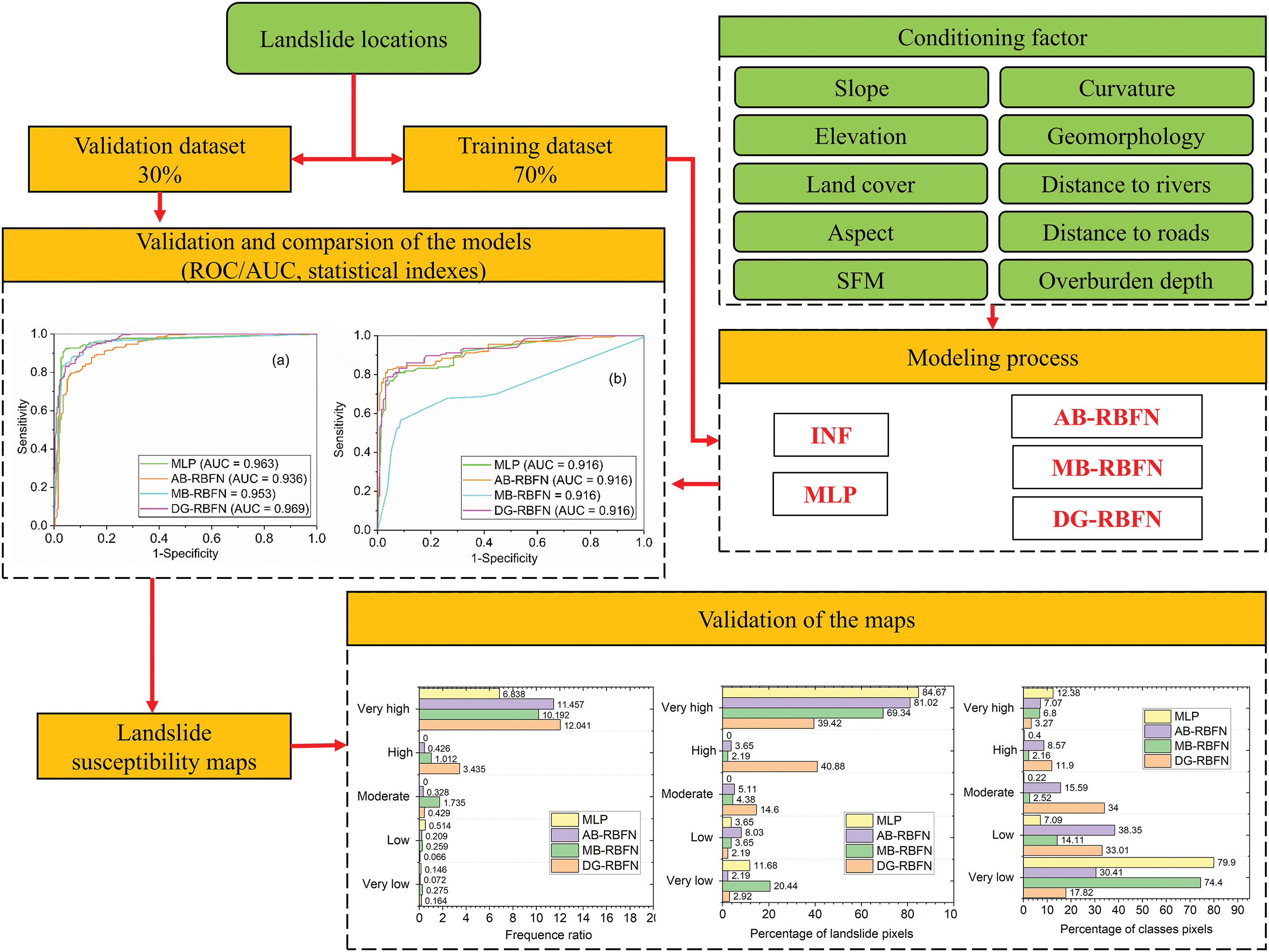
Figure 4: Methodological framework for landslide susceptibility mapping in this study

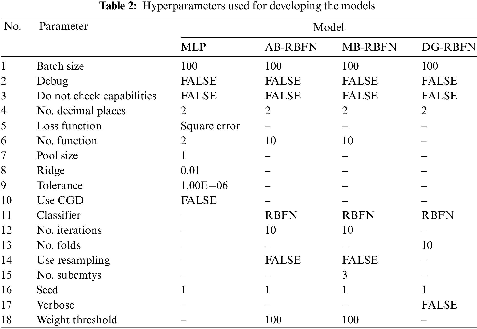
Using the training dataset, various models, including MLP, AB-RBFN, MB-RBFN, and DG-RBFN, were trained and constructed. The single MLP and the ensemble AB-RBFN, MB-RBFN, and DG-RBFN models were developed based on the hyperparameters outlined in Table 2. Each hyperparameter value was fine-tuned through a trial-and-error procedure [68].

Subsequently, these models were validated and compared against the single MLP model using established validation methods. Finally, landslide susceptibility maps were generated utilizing the outputs from the various models.

3  Results and Discussion

3.1 Factor Evaluation

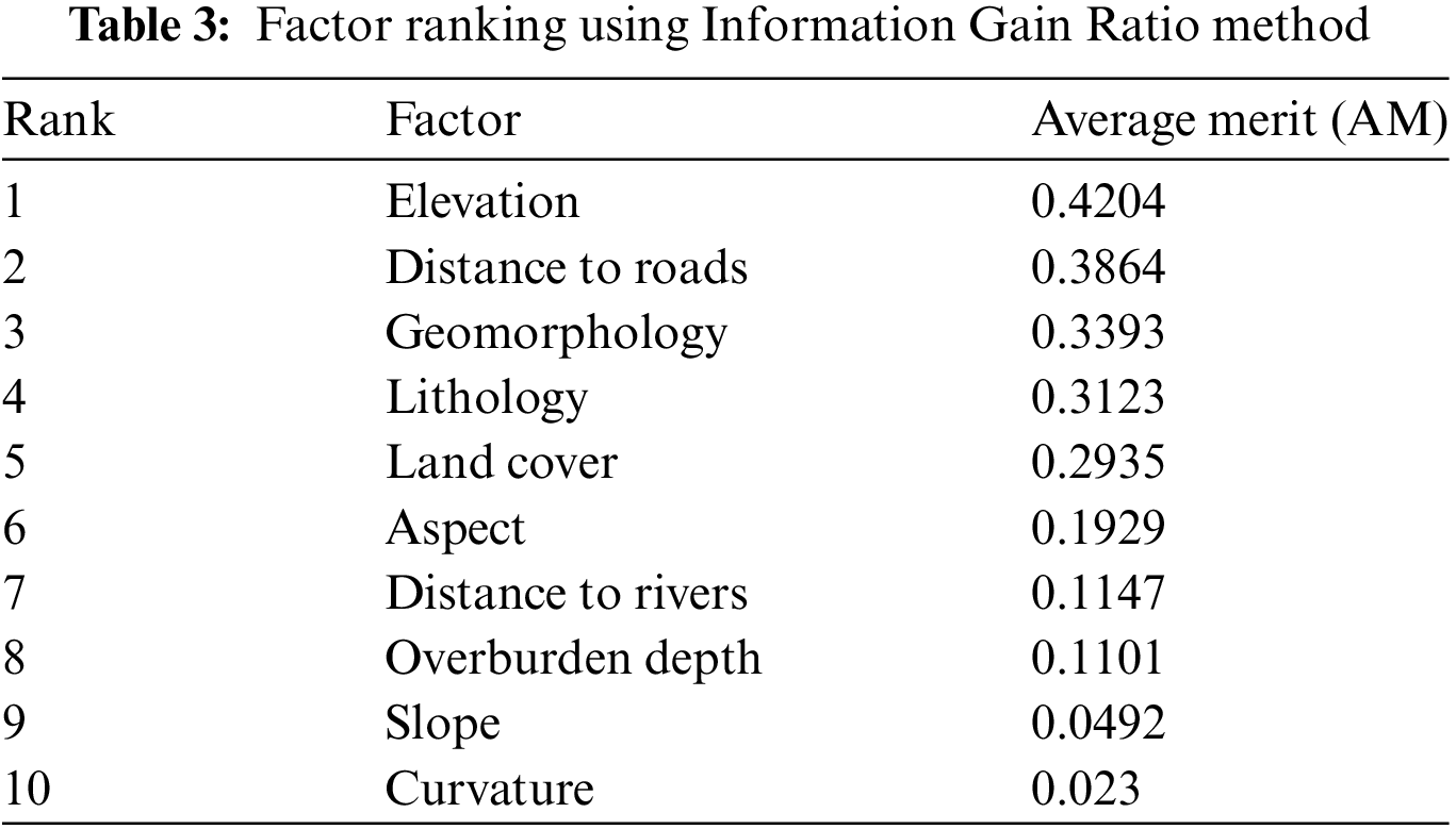
The results of the correlation and feature selection analyses are presented in Fig. 5 and Table 3. It can be seen that all selected conditioning factors are lowly correlated as the correlation values between factors are smaller than 0.5 (Fig. 5). Additionally, Table 3 demonstrates that each factor contributes to the predictive capability of the models, leading to the decision to include all of them in the landslide susceptibility modeling for this study. The factor evaluation results further highlight the significance of each factor in the modeling process. Among the selected factors, elevation shows the highest contribution to the model, with an average measure (AM) of 0.4204. This is followed by distance to roads (AM = 0.3864), geomorphology (AM = 0.3393), lithology (AM = 0.3123), land cover (AM = 0.2935), aspect (AM = 0.4204), distance to rivers (AM = 0.1929), overburden depth (AM = 0.1101), slope (AM = 0.0492), and curvature (AM = 0.023). These findings align with results from other published studies [69], reinforcing the importance of these conditioning factors in assessing landslide susceptibility. The comprehensive analysis underscores the relevance of these variables in understanding and predicting landslide occurrences, thereby providing valuable insights for effective risk management and mitigation strategies.

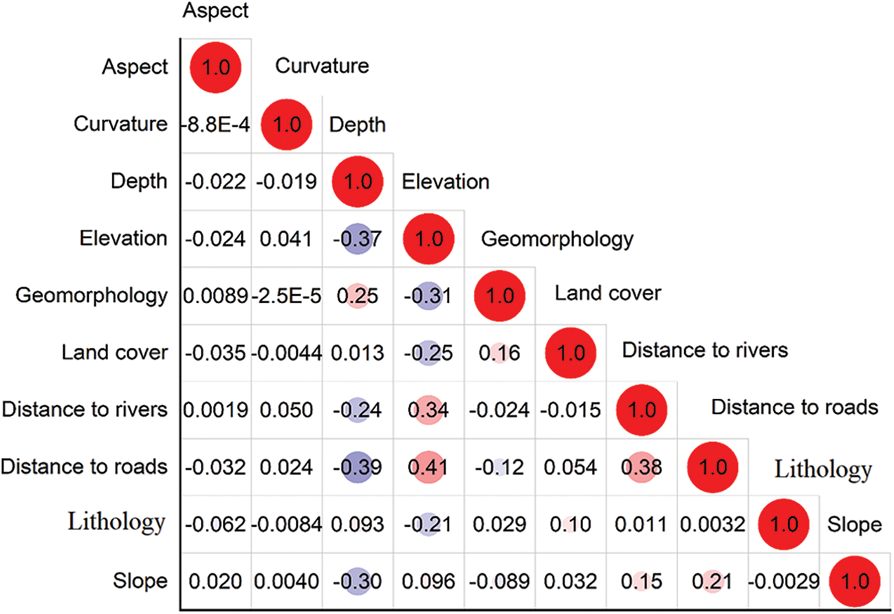
Figure 5: Correlation matrix of the landslide conditioning factors used in this study

To analyze the spatial relationship between landslide conditioning factors and past and present landslide occurrences, the Information Value (IV) method was applied. This method calculates the IV for all classes of each factor map, indicating the probability of a past or present landslide in each class and throughout the entire area (Table 4). The IV values provide insights into the influence and contribution of each factor class to landslide occurrence. Positive IV values suggest greater influence or the presence of a factor with significant contribution to landslide occurrence, while negative values indicate less influence or the presence of a factor with less significant contribution.

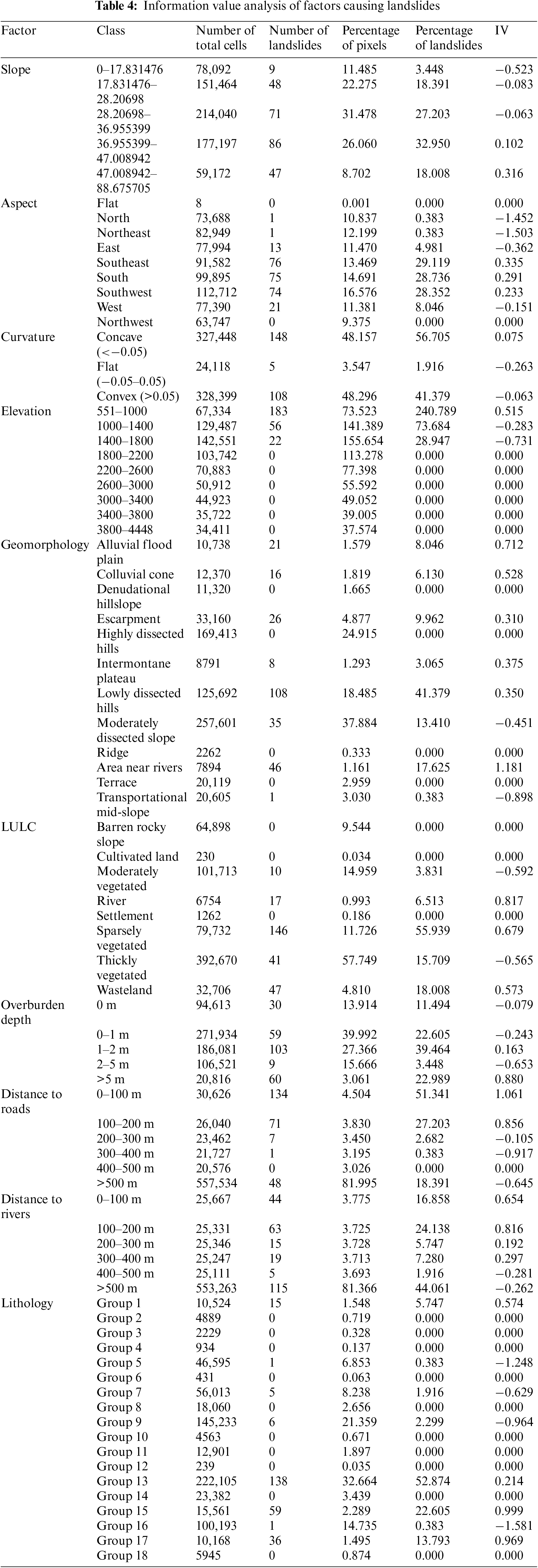
The analysis reveals that areas near rivers in geomorphology, overburden depth greater than 5 m, and a distance of 1–2 m from roads contribute the most to landslide occurrences. This is followed by alluvial flood plains in geomorphology. Other key contributors include group 17 (alluvium) in lithology, slopes ranging from 47–88°, concave regions with a curvature less than 0.05, elevations between 551–1000 m, and southeast-facing aspects. These findings align with the understanding that factors such as proximity to water bodies, thick overburden, road construction, and certain slope characteristics can significantly increase the risk of landslides.

In the modeling process, the IV values of each class for each factor (Table 4) were used to normalize the data employed for training the machine learning models. This normalization ensures that the models give appropriate weight to the different factor classes based on their relative contribution to landslide occurrence, ultimately improving the accuracy and reliability of the landslide susceptibility assessments.

3.2 Model Validation and Comparison

Validation results are shown in Table 5, Figs. 6, and 8a. It can be seen that the MLP model has the highest value of PPV (95%), followed by the AB-RBFN (89.23%), the MB-RBFN (88.85%), and the DG-RBFN (88.46%), respectively; the MLP also received the highest value of NPV (92.34%), followed by the DG-RBFN (91.95%), the MB-RBFN (88.89%), and the AB-RBFN (82.76%), respectively; the MLP received the highest value of SST (92.51%), followed by the DG-RBFN (91.63%), the MB-RBFN (88.85%), and the AB-RBFN (83.75%), respectively; the MLP received the highest value of SPF (94.88%), followed by the DG-RBFN and the MB-RBFN (88.89%), and the AB-RBFN (88.52%), respectively; the MLP had the highest value of ACC (93.67%), followed by DG-RBFN (90.21%), the MB-RBFN (88.87%), and the AB-RBFN (85.99%), respectively; the MLP had the highest value of k (0.87), followed by DG-RBFN (0.8), the MB-RBFN (0.78), and the AB-RBFN (0.72), respectively. For the RMSE, it can be seen from Fig. 6 and Table 5 that the MLP received the lowest value (0.24), followed by the DG-RBFN (0.27), the MB-RBFN (0.32), and the AB-RBFN (0.33), respectively. Using the ROC curve analysis, it can be seen from Fig. 8a that the DG-RBFN received the highest value of AUC (0.969), followed by the MLP (0.963), the MB-RBFN (0.953), and the AB-RBFN (0.936), respectively.

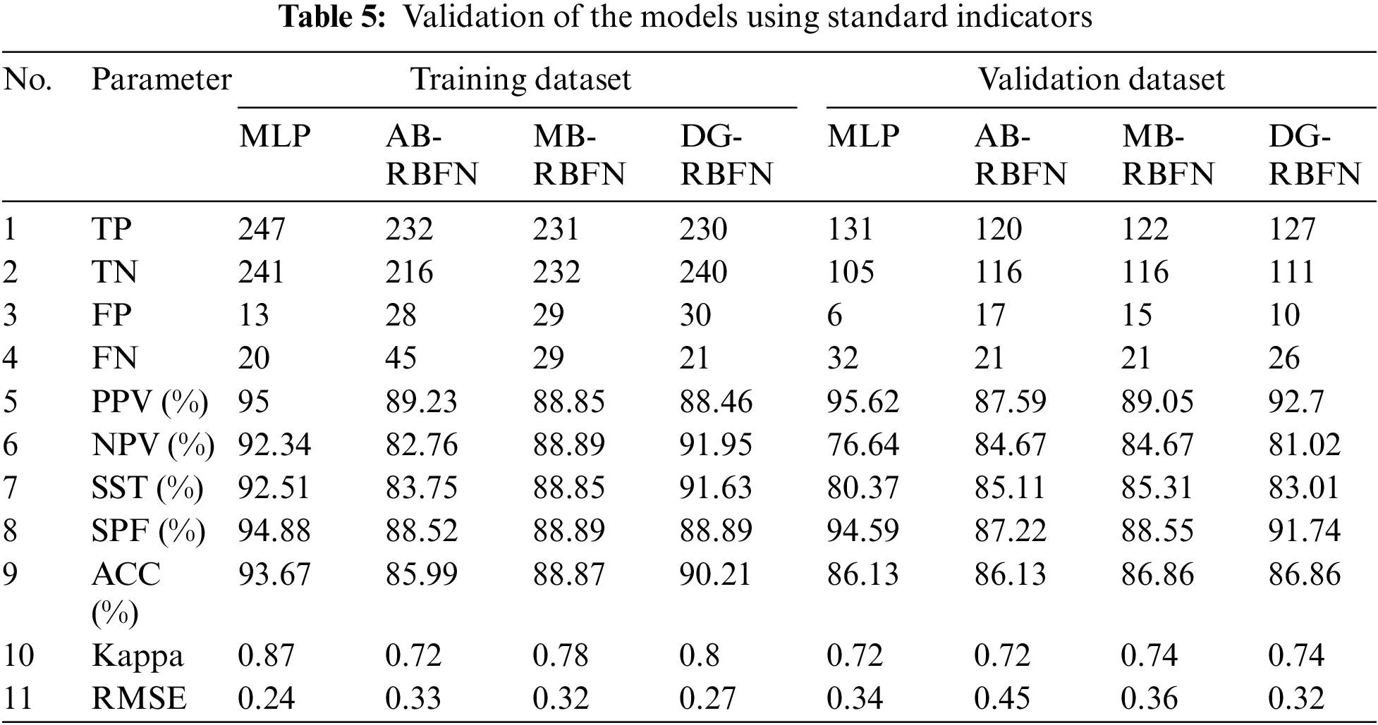
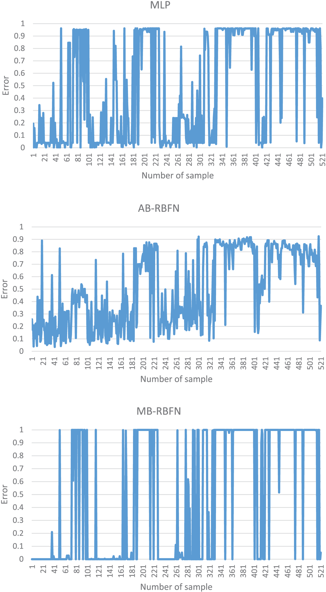
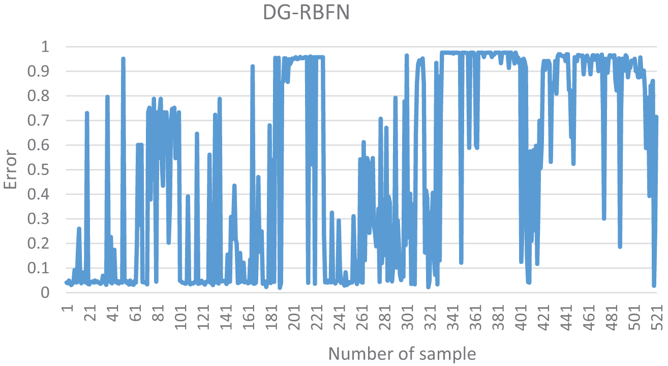
Figure 6: Error distribution of the models using training dataset

Validation of the predictive capability of the models on the validation dataset was carried out as shown in Table 5, Figs. 7, and 8b. It can be seen that the MLP model has the highest value of PPV (95.62%), followed by the DG-RBFN (92.7%), the MB-RBFN (89.05%), and the AB-RBFN (87.59%), respectively; the MB-RBFN and the AB-RBFN also received the highest value of NPV (84.67%), followed by the DG-RBFN (81.02%), and the MLP (76.64%), respectively; the MB-RBFN received the highest value of SST (85.31%), followed by the AB-RBFN (85.11%), the DG-RBFN (83.01%), and the MLP (80.37%), respectively; the MLP received the highest value of SPF (94.59%), followed by the DG-RBFN (91.74%), the MB-RBFN (88.55%), and the AB-RBFN (87.22%), respectively; the DG-RBFN and the MB-RBFN had the highest values of ACC (86.86%) compared with the AB-RBFN and the MLP (86.13%); the DG-RBFN and the MB-RBFN had the highest value of k (0.74) compared with the AB-RBFN and the MLP (0.72). For the RMSE, it can be seen from Fig. 6 and Table 5 that the DG-RBFN received the lowest value (0.32), followed by the MLP (0.34), the MB-RBFN (0.36), and the AB-RBFN (0.45), respectively. The ROC curve analysis, as illustrated in Fig. 8b, indicates that the DG-RBFN model achieved the highest area under the curve (AUC) value of 0.931. This was closely followed by the AB-RBFN model with an AUC of 0.929, the MLP model at 0.926, and the MB-RBFN model with an AUC of 0.913.

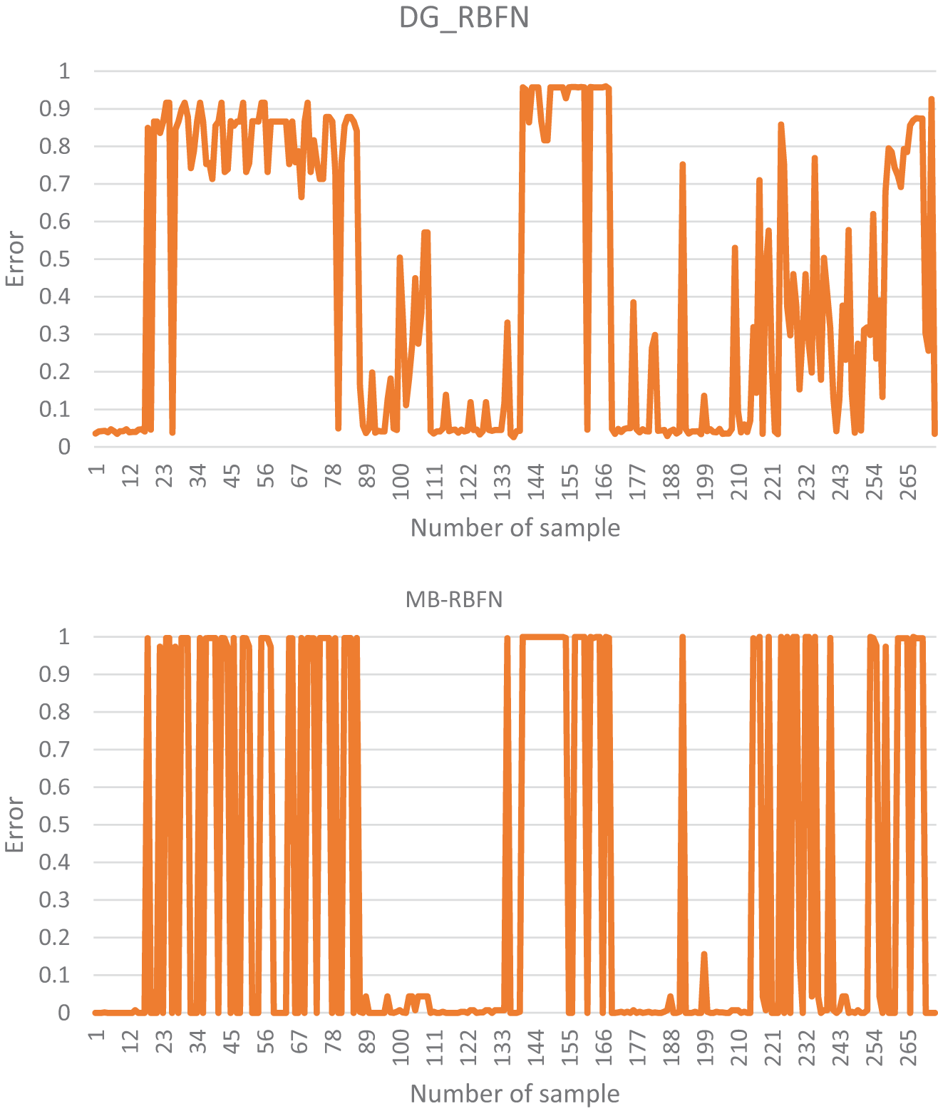
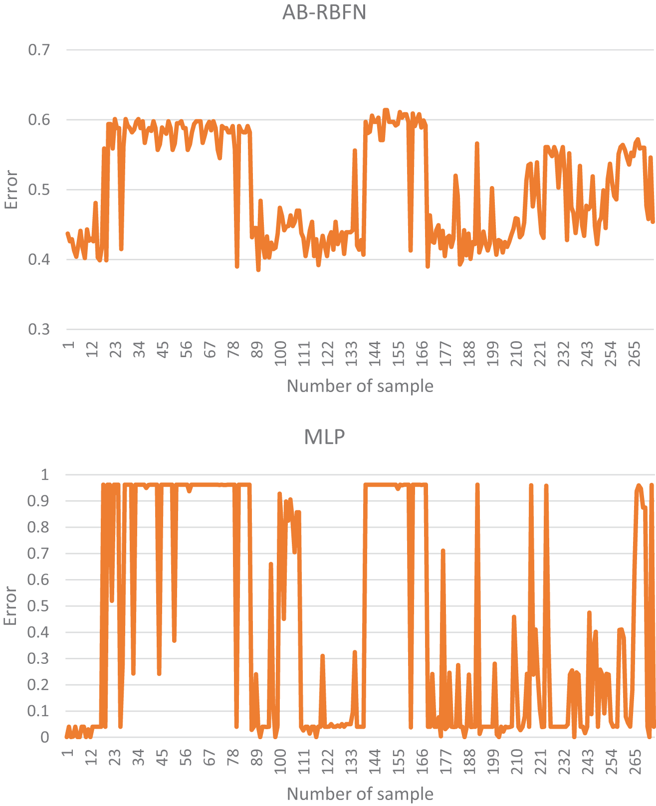
Figure 7: Error distribution of the models using validation dataset

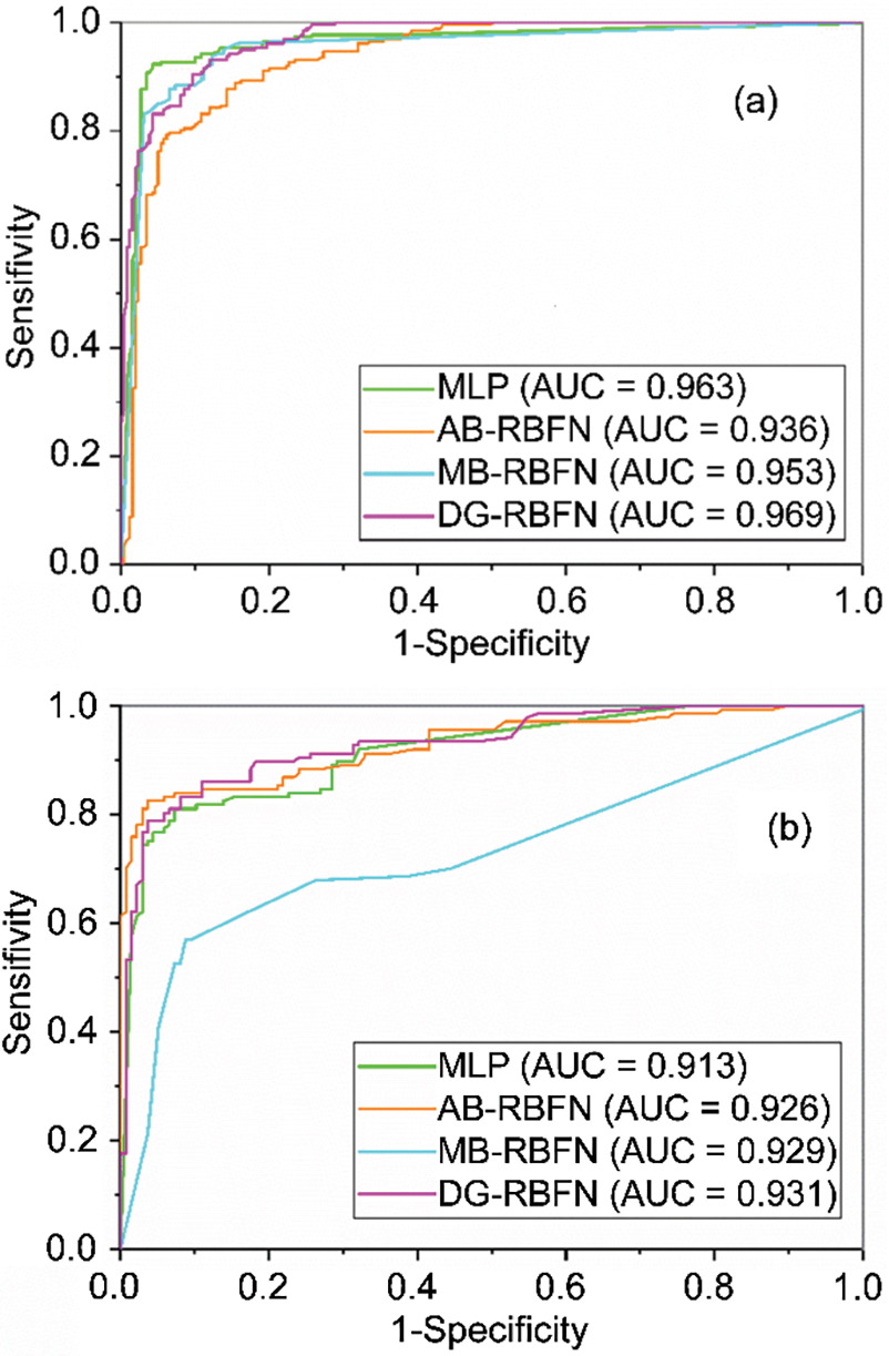
Figure 8: AUC values of the models during the (a) training phase and (b) validation phase presented at a 95% confidence interval of the classification

Based on the above analysis of the validation results of the models, it can be stated that all models used in this study are good for prediction of landslide susceptibility, but the DG-RBFN is better than other models (MLP, AB-RBFN, and MB-RBFN). It is reasonable as the DG-RBFN received the supports from the DG optimization for improving the performance of the landslide modeling. More specifically, the advantages of the DG include [70–72]: (i) Improved prediction accuracy: it often outperforms individual classifiers by reducing overfitting and improving generalization. The combination of diverse classifiers can capture a broader range of patterns and increase overall prediction accuracy, (ii) Reducing overfitting: By using multiple classifiers that are trained on different subsets of the data, it can reduce the likelihood of overfitting. Each classifier focuses on different aspects of the data, and their combination helps to smooth out the noise and capture the underlying patterns, (iii) Enhanced robustness: it can improve the robustness of the predictions. By combining multiple classifiers, the ensemble becomes more resilient to outliers, noise, or errors in individual classifiers. The ensemble’s decision is based on a consensus among its members, reducing the impact of individual errors, (iv) Handling class imbalance: it can be particularly effective when dealing with imbalanced datasets. By using different subsets of data for training each classifier, it provides an opportunity to balance the representation of minority classes and improve their classification performance. In addition, it’s important to note that the effectiveness of DG ensembles depends on the diversity and quality of the individual classifiers. In this study, the RBFN is proved as a great classifier for combining with the DG in the ensemble model (DG-RBFN) for prediction of landslide susceptibility. Compared with other optimization techniques like AB and MB, the DG is superior in reducing correlation between classifiers in the ensemble framework. As a result, it can improve and enhance the performance of the ensemble model [71]. In addition, the performance of the novel hybrid model DG-RBFN is better than single RBFN, Logistic Regression (LR), Linear Discriminant Analysis (LDA) and Alternating Decision Tree (ADT), Naïve Bayes (NB) [73] when applied in the similar areas.

3.3 Susceptibility Map Construction

The process of generating landslide susceptibility maps involved training the machine learning models using a training dataset, followed by calculating Landslide Susceptibility Indices (LSI) for all pixels within the study area using the trained models. To facilitate interpretation, the geometrical intervals (GI) classification method was employed to categorize the LSI values into five distinct classes (Fig. 9).

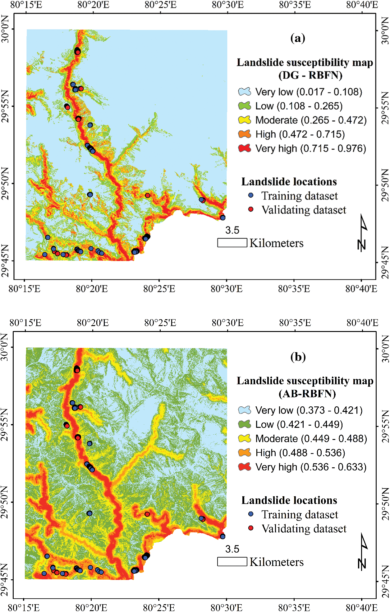
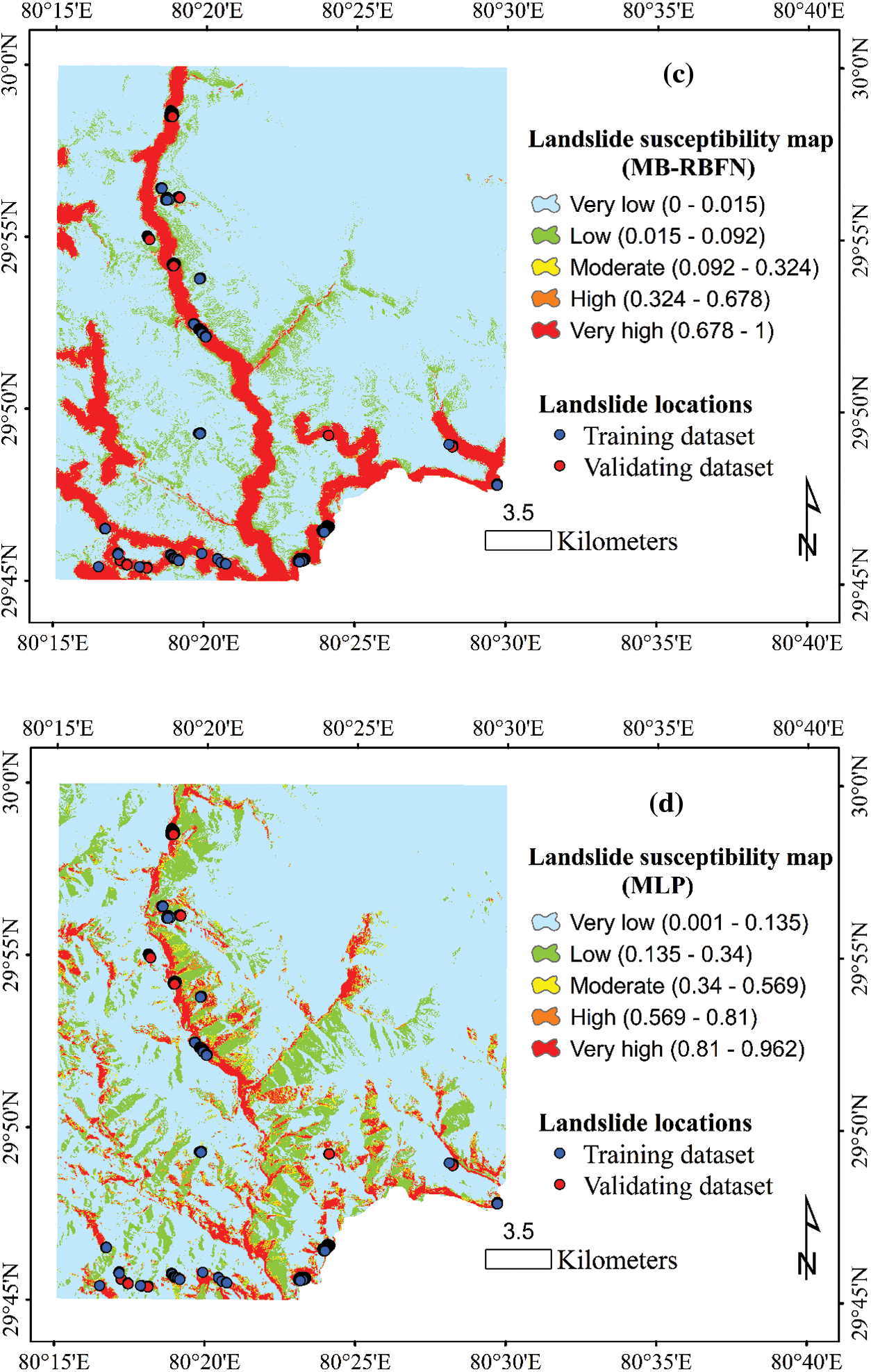
Figure 9: Landslide susceptibility maps produced using the (a) DG-RBFN, (b) AB-RBFN, (c) MB-RBFN, and (d) MLP models

Validating the accuracy of the susceptibility maps generated by the models was accomplished by computing the frequency ratio (FR) of landslide pixels within each susceptibility class (Fig. 10). The results of the analysis revealed that the very high susceptibility class in all the susceptibility maps generated by the models exhibits the highest FR values compared to the other classes (very low, low, moderate, high). This finding suggests that the majority of historical landslides are located within the very high susceptibility class of the maps, indicating the reliability of the models for practical applications. Furthermore, the FR value for the very high susceptibility class of the map generated by the DG-RBFN model (12.041) is notably higher than those of the other models (MLP, AB-RBFN, MB-RBFN). This observation leads to the conclusion that the map produced by the DG-RBFN model is superior to the maps generated by the other models in terms of accurately predicting landslide susceptibility.

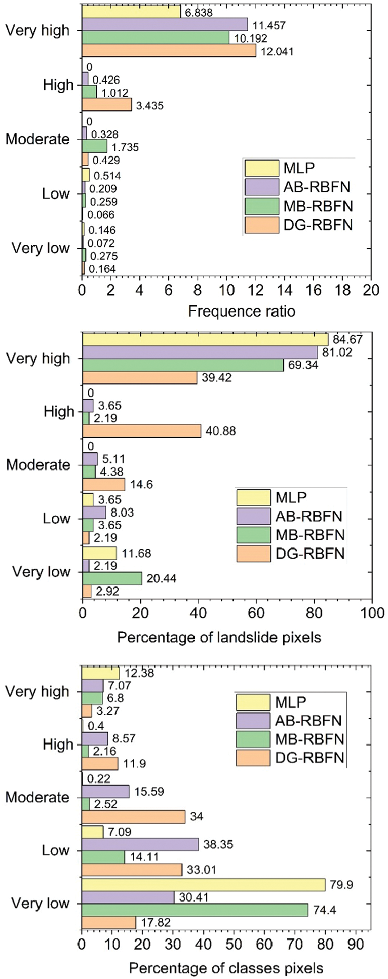
Figure 10: Analysis of FR on the susceptibility maps using the models

3.4 Implications, Limitations, and Recommendations

The novel ensemble models developed in this study, particularly the DG-RBFN, have demonstrated exceptional performance in predicting landslide susceptibility in the Pithoragarh region of Uttarakhand, India. However, the true versatility and potential impact of these models lie in their ability to be adapted and applied to other regions with varying geological conditions. By incorporating different sets of landslide conditioning factors relevant to the target area, these models can be easily trained and validated to produce accurate susceptibility maps for diverse landscapes. One of the key advantages of the DG-RBFN model is its ability to handle complex, non-linear relationships between landslide occurrence and conditioning factors. This makes it particularly suitable for regions with heterogeneous geological settings, where the factors influencing landslides may vary significantly. For instance, in areas with a predominance of sedimentary rocks, factors such as bedding plane orientation and rock strength may play a crucial role, while in volcanic regions, factors like fracture density and weathering intensity may be more important [74]. The DG-RBFN’s flexibility allows it to capture these nuances and produce reliable susceptibility assessments.

However, it is important to note that while the proposed models have shown promising results, they are not without limitations. As “black box” models, they do not provide direct insights into the underlying mechanisms driving landslides. To address this, future research should focus on integrating the DG-RBFN with techniques like SHAP (Shapley Additive Explanations) to enhance the interpretability of the models and gain a better understanding of the relative importance of each conditioning factor in different geological settings. Moreover, the performance of these models is heavily dependent on the quality and quantity of the input data. The limited availability of data may have led to issues such as overfitting, which can be mitigated by using larger datasets or employing techniques like cross-validation [11]. Future work should prioritize collecting comprehensive datasets, including detailed surface and subsurface geological information, long-term meteorological records, and high-resolution remote sensing data, to improve the reliability and robustness of the models. Despite these limitations, the DG-RBFN and other ensemble models developed in this study hold immense potential for revolutionizing landslide susceptibility assessment worldwide. By adapting these models to local conditions and incorporating cutting-edge techniques for data collection and analysis, researchers and practitioners can contribute to more effective disaster risk reduction strategies, ultimately saving lives and minimizing economic losses.

4  Conclusion

We have developed and validated the performance of novel ensemble models, namely DG-RBFN, MB-RBFN, and AB-RBFN, alongside the single MLP ML model. These models were applied to a dataset (261 historical landslide occurrences and ten conditioning factors) sourced from a landslide-prone region in Pithoragarh, Uttarakhand, India. Utilizing standard evaluation metrics, we analyzed the models’ training and performances. Our findings indicated that all models demonstrated strong predictive capabilities for landslide susceptibility. Notably, the DG-RBFN model excelled, achieving an AUC of 0.931, surpassing the performance of the other models. Consequently, we conclude that the DG-RBFN model is a robust and effective tool for assessing landslide susceptibility, with the potential for application in other vulnerable regions globally.

The landslide susceptibility map produced by the DG-RBFN ensemble model serves as a vital resource for a diverse range of stakeholders, including planners, engineers, policymakers, and the general public. By identifying regions that are particularly vulnerable to landslides, this map can significantly inform decision-making processes related to land use planning, infrastructure development, disaster mitigation strategies, and emergency response planning. Understanding the areas most at risk can help authorities implement proactive measures to minimize hazards. For instance, they can establish zoning regulations to restrict construction in high-risk zones, construct retaining walls to stabilize slopes and engage in other engineering practices designed to mitigate potential landslide impacts. While the ensemble models developed in this study have been effectively trained and validated, it is crucial to acknowledge their inherent limitations as black box models. This means that their decision-making processes are not easily interpretable, particularly when it comes to evaluating landslide susceptibility. To enhance our understanding of these models, it is recommended that the SHAP technique be employed. This approach can provide insights into the contributions of various features to the model’s predictions, thereby improving transparency and trust in the results. Moreover, the performance of models can be influenced by uncertainties stemming from the complex nature of geological and geo-environmental processes that contribute to landslides. To mitigate these uncertainties, comprehensive surface and subsurface geological investigations are essential. Additionally, the availability of reliable time series meteorological data and extensive remote sensing data, including DEMs and satellite imagery, can enhance model accuracy. Additionally, combining multiple models and relying on confidence intervals can further enhance model robustness. Many of these strategies have been implemented in this study; however, it would be advantageous to select a study area with a larger dataset for ensemble modeling. Doing so would reduce the risk of overfitting and diminish the necessity for compensatory techniques, ultimately leading to more reliable and generalizable results in landslide susceptibility assessments.

Acknowledgement: We are grateful to the anonymous reviewers whose comments significantly improved this manuscript.

Funding Statement: This research is funded by the University of Transport Technology under the project entitled “Application of Machine Learning Algorithms in Landslide Susceptibility Mapping in Mountainous Areas” with grant number DTTD2022-16.

Author Contributions: The authors confirm contribution to the paper as follows: study conception and design: Duc-Dam Nguyen, Nguyen Viet Tiep, Binh Thai Pham; data collection: Duc-Dam Nguyen, Binh Thai Pham, Hiep Van Le; analysis and interpretation of results: Duc-Dam Nguyen, Nguyen Viet Tiep, Binh Thai Pham, Indra Prakash; draft manuscript preparation: all authors. All authors reviewed the results and approved the final version of the manuscript.

Availability of Data and Materials: The data that support the findings of this study are available from the corresponding author, Nguyen Viet Tiep, upon reasonable request.

Ethics Approval: Not applicable.

Conflicts of Interest: The authors declare no conflicts of interest to report regarding the present study.

References

1. Teknős L. Analysis and assessment of the growing tendencies of natural disasters and events in Hungary from the perspective of disaster management. Secur Dimens. 2022;43(43):53–75. doi:10.5604/01.3001.0054.1483. [Google Scholar] [CrossRef]

2. Alimonti G, Mariani L. Is the number of global natural disasters increasing? Environ Haz. 2024;23(2):186–202. doi:10.1080/17477891.2023.2239807. [Google Scholar] [CrossRef]

3. Bukhari MH, da Silva PF, Pilz J, Istanbulluoglu E, Görüm T, Lee J, et al. Community perceptions of landslide risk and susceptibility: a multi-country study. Landslides. 2023;20(6):1321–34. doi:10.1007/s10346-023-02027-5. [Google Scholar] [CrossRef]

4. Pham QB, Achour Y, Ali SA, Parvin F, Vojtek M, Vojteková J, et al. A comparison among fuzzy multi-criteria decision making, bivariate, multivariate and machine learning models in landslide susceptibility mapping. Geomatics, Nat Hazards Risk. 2021;12(1):1741–77. doi:10.1080/19475705.2021.1944330. [Google Scholar] [CrossRef]

5. Chowdhury MS, Rahaman MN, Sheikh MS, Sayeid MA, Mahmud KH, Hafsa B. GIS-based landslide susceptibility mapping using logistic regression, random forest and decision and regression tree models in Chattogram District, Bangladesh. Heliyon. 2024;10(1):e23424. doi:10.1016/j.heliyon.2023.e23424. [Google Scholar] [PubMed] [CrossRef]

6. Huang Y, Zhao L. Review on landslide susceptibility mapping using support vector machines. Catena. 2018;165:520–9. doi:10.1016/j.catena.2018.03.003. [Google Scholar] [CrossRef]

7. Jaafari A. Landslide susceptibility assessment using novel hybridized methods based on the support vector regression. Ecol Eng. 2024;208:107372. doi:10.1016/j.ecoleng.2024.107372. [Google Scholar] [CrossRef]

8. Kalantar B, Pradhan B, Naghibi SA, Motevalli A, Mansor S. Assessment of the effects of training data selection on the landslide susceptibility mapping: a comparison between support vector machine (SVMlogistic regression (LR) and artificial neural networks (ANN). Geomat Nat Hazards Risk. 2018;9(1):49–69. doi:10.1080/19475705.2017.1407368. [Google Scholar] [CrossRef]

9. Teke A, Kavzoglu T. Exploring the decision-making process of ensemble learning algorithms in landslide susceptibility mapping: insights from local and global explainable AI analyses. Adv Space Res. 2024;74(8):3765–85. doi:10.1016/j.asr.2024.06.082. [Google Scholar] [CrossRef]

10. Jaafari A, Panahi M, Pham BT, Shahabi H, Bui DT, Rezaie F, et al. Meta optimization of an adaptive neuro-fuzzy inference system with grey wolf optimizer and biogeography-based optimization algorithms for spatial prediction of landslide susceptibility. Catena. 2019;175:430–45. doi:10.1016/j.catena.2018.12.033. [Google Scholar] [CrossRef]

11. Jaafari A, Panahi M, Mafi-Gholami D, Rahmati O, Shahabi H, Shirzadi A, et al. Swarm intelligence optimization of the group method of data handling using the cuckoo search and whale optimization algorithms to model and predict landslides. Appl Soft Comput. 2022;116(10):108254. doi:10.1016/j.asoc.2021.108254. [Google Scholar] [CrossRef]

12. Ren T, Gao L, Gong W. An ensemble of dynamic rainfall index and machine learning method for spatiotemporal landslide susceptibility modeling. Landslides. 2024;21(2):257–73. doi:10.1007/s10346-023-02152-1. [Google Scholar] [CrossRef]

13. Di Napoli M, Carotenuto F, Cevasco A, Confuorto P, Di Martire D, Firpo M, et al. Machine learning ensemble modelling as a tool to improve landslide susceptibility mapping reliability. Landslides. 2020;17(8):1897–914. doi:10.1007/s10346-020-01392-9. [Google Scholar] [CrossRef]

14. Hong H, Liu J, Zhu A-X. Modeling landslide susceptibility using LogitBoost alternating decision trees and forest by penalizing attributes with the bagging ensemble. Sci Tot Environ. 2020;718(18):137231. doi:10.1016/j.scitotenv.2020.137231. [Google Scholar] [PubMed] [CrossRef]

15. Pham BT, Jaafari A, Nguyen-Thoi T, Van Phong T, Nguyen HD, Satyam N, et al. Ensemble machine learning models based on Reduced Error Pruning Tree for prediction of rainfall-induced landslides. Int J Digit Earth. 2020;14(5):575–96. doi:10.1080/17538947.2020.1860145. [Google Scholar] [CrossRef]

16. Lv L, Chen T, Dou J, Plaza A. A hybrid ensemble-based deep-learning framework for landslide susceptibility mapping. Int J Appl Earth Obser Geoinform. 2022;108:102713. doi:10.1016/j.jag.2022.102713. [Google Scholar] [CrossRef]

17. Bien TX, Truyen PT, Phong TV, Nguyen DD, Amiri M, Costache R, et al. Landslide susceptibility mapping at sin Ho, Lai Chau province, Vietnam using ensemble models based on fuzzy unordered rules induction algorithm. Geo Int. 2022;37(27):17777–98. [Google Scholar]

18. Saha S, Roy J, Pradhan B, Hembram TK. Hybrid ensemble machine learning approaches for landslide susceptibility mapping using different sampling ratios at East Sikkim Himalayan, India. Adv Space Res. 2021;68(7):2819–40. doi:10.1016/j.asr.2021.05.018. [Google Scholar] [CrossRef]

19. Tran QC, Minh DD, Jaafari A, Al-Ansari N, Minh DD, Van DT, et al. Novel ensemble landslide predictive models based on the Hyperpipes Algorithm: a case study in the Nam Dam Commune, Vietnam. Appl Sci. 2020;10(11):3710. doi:10.3390/app10113710. [Google Scholar] [CrossRef]

20. Pham BT, Jaafari A, Nguyen DD, Bayat M, Nguyen HBT. Development of multiclass alternating decision trees based models for landslide susceptibility mapping. Phys Chem Earth. 2022;128:103235. doi:10.1016/j.pce.2022.103235. [Google Scholar] [CrossRef]

21. Hong H. Assessing landslide susceptibility based on hybrid Best-first decision tree with ensemble learning model. Ecol Ind. 2023;147:109968. doi:10.1016/j.ecolind.2023.109968. [Google Scholar] [CrossRef]

22. Le Minh N, Truyen PT, Van Phong T, Jaafari A, Amiri M, Van Duong N, et al. Ensemble models based on radial basis function network for landslide susceptibility mapping. Environ Sci Pollut Res. 2023;30(44):99380–98. doi:10.1007/s11356-023-29378-9. [Google Scholar] [PubMed] [CrossRef]

23. Adnan MSG, Rahman MS, Ahmed N, Ahmed B, Rabbi MF, Rahman RM. Improving spatial agreement in machine learning-based landslide susceptibility mapping. Rem Sens. 2020;12(20):3347. doi:10.3390/rs12203347. [Google Scholar] [CrossRef]

24. Rossi M, Guzzetti F, Reichenbach P, Mondini AC, Peruccacci S. Optimal landslide susceptibility zonation based on multiple forecasts. Geomorphology. 2010;114(3):129–42. doi:10.1016/j.geomorph.2009.06.020. [Google Scholar] [CrossRef]

25. Sterlacchini S, Ballabio C, Blahut J, Masetti M, Sorichetta A. Spatial agreement of predicted patterns in landslide susceptibility maps. Geomorphology. 2011;125(1):51–61. doi:10.1016/j.geomorph.2010.09.004. [Google Scholar] [CrossRef]

26. Guzzetti F, Reichenbach P, Ardizzone F, Cardinali M, Galli M. Estimating the quality of landslide susceptibility models. Geomorphology. 2006;81(1–2):166–84. doi:10.1016/j.geomorph.2006.04.007. [Google Scholar] [CrossRef]

27. Gu X, Li Y, Zuo X, Bu J, Yang F, Yang X, et al. Image compression-based DS-InSAR method for landslide identification and monitoring of alpine canyon region: a case study of Ahai Reservoir area in Jinsha River Basin. Landslides. 2024;21(10):1–17. doi:10.1007/s10346-024-02299-5. [Google Scholar] [CrossRef]

28. Pham BT, Jaafari A, Van Phong T, Mafi-Gholami D, Amiri M, Van Tao N, et al. Naïve Bayes ensemble models for groundwater potential mapping. Ecolo Inf. 2021;64:101389. doi:10.1016/j.ecoinf.2021.101389. [Google Scholar] [CrossRef]

29. Ngo TQ, Dam ND, Al-Ansari N, Amiri M, Phong TV, Prakash I, et al. Landslide susceptibility mapping using single machine learning models: a case study from Pithoragarh District, India. Adv Civ Eng. 2021;2021(1):9934732. doi:10.1155/2021/9934732. [Google Scholar] [CrossRef]

30. Du W, Wang G. Fully probabilistic seismic displacement analysis of spatially distributed slopes using spatially correlated vector intensity measures. Earthquake Eng Struct Dyn. 2014;43(5):661–79. doi:10.1002/eqe.2365. [Google Scholar] [CrossRef]

31. Liu G, Meng H, Song G, Bo W, Zhao P, Ning B, et al. Numerical simulation of wedge failure of rock slopes using three-dimensional discontinuous deformation analysis. Environ Earth Sci. 2024;83(10):310. doi:10.1007/s12665-024-11619-w. [Google Scholar] [CrossRef]

32. Zhou G, Xu J, Hu H, Liu Z, Zhang H, Xu C, et al. Off-axis four-reflection optical structure for lightweight single-band bathymetric LiDAR. IEEE Trans Geosci Rem Sens. 2023;61:1000917. doi:10.1109/TGRS.2023.3298531. [Google Scholar] [CrossRef]

33. Zhou G, Lin G, Liu Z, Zhou X, Li W, Li X, et al. An optical system for suppression of laser echo energy from the water surface on single-band bathymetric LiDAR. Opt Lasers Eng. 2023;163(8):107468. doi:10.1016/j.optlaseng.2022.107468. [Google Scholar] [CrossRef]

34. Burnett BN, Meyer GA, McFadden LD. Aspect-related microclimatic influences on slope forms and processes, Northeastern Arizona. J Geophys Res: Earth Surf. 2008;113(F3):29. doi:10.1029/2007JF000789. [Google Scholar] [CrossRef]

35. Chen W, Li Y. GIS-based evaluation of landslide susceptibility using hybrid computational intelligence models. Catena. 2020;195:104777. doi:10.1016/j.catena.2020.104777. [Google Scholar] [CrossRef]

36. Zhao Y, Li J, Tian Y, Li J. Distinguish extreme precipitation mechanisms associated with atmospheric river and non-atmospheric river in the Lower Yangtze River Basin. J Climate. 2024;37(15):3995–4010. doi:10.1175/JCLI-D-23-0400.1. [Google Scholar] [CrossRef]

37. Zhang J, Wang S, Huang J, He Y, Ren Y. The precipitation-recycling process enhanced extreme precipitation in Xinjiang, China. Geophys Res Lett. 2023;50(15):e2023GL104324. doi:10.1029/2023GL104324. [Google Scholar] [CrossRef]

38. Zhou G, Tang Y, Zhang W, Liu W, Jiang Y, Gao E, et al. Shadow detection on high-resolution digital orthophoto map (DOM) using semantic matching. IEEE Trans Geosci Rem Sens. 2023;61:1–20. doi:10.1109/TGRS.2023.3336053. [Google Scholar] [CrossRef]

39. Nhu V-H, Mohammadi A, Shahabi H, Shirzadi A, Al-Ansari N, Ahmad BB, et al. Monitoring and assessment of water level fluctuations of the lake urmia and its environmental consequences using multitemporal landsat 7 ETM+ images. Int J Environ Res Public Health. 2020;17(12):4210. doi:10.3390/ijerph17124210. [Google Scholar] [PubMed] [CrossRef]

40. Ye X, Zhu H-H, Chang F-N, Xie T-C, Tian F, Zhang W, et al. Revisiting spatiotemporal evolution process and mechanism of a giant reservoir landslide during weather extremes. Eng Geol. 2024;332(3):107480. doi:10.1016/j.enggeo.2024.107480. [Google Scholar] [CrossRef]

41. Ye B, Qiu H, Tang B, Liu Y, Liu Z, Jiang X, et al. Creep deformation monitoring of landslides in a reservoir area. J Hydrol. 2024;632(16):130905. doi:10.1016/j.jhydrol.2024.130905. [Google Scholar] [CrossRef]

42. Wu L, He B, Peng J. Analysis of rainfall-caused seepage into underlying bedrock slope based on seepage deformation coupling. Int J Geomech. 2024;24(5):04024076. doi:10.1061/IJGNAI.GMENG-9175. [Google Scholar] [CrossRef]

43. Qiu H, Su L, Tang B, Yang D, Ullah M, Zhu Y, et al. The effect of location and geometric properties of landslides caused by rainstorms and earthquakes. Earth Surf Process Landf. 2024;49(7):2067–79. doi:10.1002/esp.5816. [Google Scholar] [CrossRef]

44. Liu C, Shan Y, He L, Li F, Liu X, Nepf H. Plant morphology impacts bedload sediment transport. Geophys Res Lett. 2024;51(12):e2024GL108800. doi:10.1029/2024GL108800. [Google Scholar] [CrossRef]

45. Gallardo-Salazar JL, Rosas-Chavoya M, Pompa-García M, López-Serrano PM, García-Montiel E, Meléndez-Soto A, et al. Multi-temporal NDVI analysis using UAV images of tree crowns in a northern Mexican pine-oak forest. J For Res. 2023;34(6):1855–67. doi:10.1007/s11676-023-01639-w. [Google Scholar] [CrossRef]

46. Ma K, Peng Y, Liao Z, Wang Z. Dynamic responses and failure characteristics of the tunnel caused by rockburst: an entire process modelling from incubation to occurrence phases. Comput Geotech. 2024;171:106340. doi:10.1016/j.compgeo.2024.106340. [Google Scholar] [CrossRef]

47. Jahandar O, Abdi E, Jaafari A. Assessment of slope failure susceptibility along road networks in a forested region, Northern Iran. Phys Chem Earth. 2022;128:103272. doi:10.1016/j.pce.2022.103272. [Google Scholar] [CrossRef]

48. Yin L, Wang L, Keim BD, Konsoer K, Yin Z, Liu M, et al. Spatial and wavelet analysis of precipitation and river discharge during operation of the Three Gorges Dam, China. Ecol Ind. 2023;154:110837. doi:10.1016/j.ecolind.2023.110837. [Google Scholar] [CrossRef]

49. Yin L, Wang L, Keim BD, Konsoer K, Zheng W. Wavelet analysis of dam injection and discharge in three gorges dam and reservoir with precipitation and river discharge. Water. 2022;14(4):567. doi:10.3390/w14040567. [Google Scholar] [CrossRef]

50. Van Dao D, Jaafari A, Bayat M, Mafi-Gholami D, Qi C, Moayedi H, et al. A spatially explicit deep learning neural network model for the prediction of landslide susceptibility. Catena. 2020;188:104451. doi:10.1016/j.catena.2019.104451. [Google Scholar] [CrossRef]

51. Jaafari A, Janizadeh S, Abdo HG, Mafi-Gholami D, Adeli B. Understanding land degradation induced by gully erosion from the perspective of different geoenvironmental factors. J Environ Manag. 2022;315:115181. doi:10.1016/j.jenvman.2022.115181. [Google Scholar] [PubMed] [CrossRef]

52. Sarkar S, Kanungo D, Ptra A, Kumar P. Disaster mitigation of debris flow, slope failure, and landslides. In: GIS-based landslide susceptibility case study in Indian Himalaya. Tokyo, Japan: Universal Acadamy Press; 2006. [Google Scholar]

53. Kanungo D, Arora M, Sarkar S, Gupta R. Landslide susceptibility zonation (LSZ) mapping–a review. J South Asia Disaster Studies. 2012;2(1). doi:10.1142/98127016050038_0038. [Google Scholar] [CrossRef]

54. Wubalem A, Meten M. Landslide susceptibility mapping using information value and logistic regression models in Goncha Siso Eneses area, Northwestern Ethiopia. SN Appl Sci. 2020;2:1–19. [Google Scholar]

55. Bayat M, Ghorbanpour M, Zare R, Jaafari A, Pham B. Application of artificial neural networks for predicting tree survival and mortality in the Hyrcanian forest of Iran. Comput Electron Agric. 2019;164:104929. doi:10.1016/j.compag.2019.104929. [Google Scholar] [CrossRef]

56. Du K-L, Swamy MNS. Radial basis function networks. In: Neural networks and statistical learning. London: Springer London; 2014. p. 299–335. [Google Scholar]

57. Ting KM, Witten IH. Stacking bagged and dagged models. Hamilton, New Zealand: University of Waikato; 1997. [Google Scholar]

58. Adnan RM, Jaafari A, Mohanavelu A, Kisi O, Elbeltagi A. Novel ensemble forecasting of streamflow using locally weighted learning algorithm. Sustainability. 2021;13(11):5877. doi:10.3390/su13115877. [Google Scholar] [CrossRef]

59. Moayedi H, Xu M, Naderian P, Dehrashid AA, Thi QT. Validation of four optimization evolutionary algorithms combined with artificial neural network (ANN) for landslide susceptibility mapping: a case study of Gilan, Iran. Ecol Eng. 2024;201:107214. doi:10.1007/s11069-005-5182-6. [Google Scholar] [CrossRef]

60. Beguería S. Validation and evaluation of predictive models in hazard assessment and risk management. Nat Haz. 2006;37(3):315–29. doi:10.1016/j.ecoleng.2024.107214. [Google Scholar] [CrossRef]

61. Chen W, Xie X, Peng J, Wang J, Duan Z, Hong H. GIS-based landslide susceptibility modelling: a comparative assessment of kernel logistic regression, Naïve-Bayes tree, and alternating decision tree models. Geomat Nat Hazards Risk. 2017;8(2):950–73. doi:10.1080/19475705.2017.1289250. [Google Scholar] [CrossRef]

62. Bui DT, Ho T-C, Pradhan B, Pham B-T, Nhu V-H, Revhaug I. GIS-based modeling of rainfall-induced landslides using data mining-based functional trees classifier with AdaBoost, Bagging, and MultiBoost ensemble frameworks. Environ Earth Sci. 2016;75(14):1–22. [Google Scholar]

63. Liu H, Dong X, Meng Y, Gao T, Mao L, Gao R. A novel model to evaluate spatial structure in thinned conifer-broadleaved mixed natural forests. J For Res. 2023;34(6):1881–98. doi:10.1007/s11676-023-01647-w. [Google Scholar] [CrossRef]

64. Yariyan P, Janizadeh S, Van Phong T, Nguyen HD, Costache R, Van Le H, et al. Improvement of best first decision trees using bagging and dagging ensembles for flood probability mapping. Water Resour Manag. 2020;34(9):3037–53. doi:10.1007/s11269-020-02603-7. [Google Scholar] [CrossRef]

65. Chen G, Zhang K, Wang S, Xia Y, Chao L. iHydroSlide3D v1. 0: an advanced hydrological-geotechnical model for hydrological simulation and three-dimensional landslide prediction. Geosci Model Dev. 2023;16(10):2915–37. doi:10.5194/gmd-16-2915-2023. [Google Scholar] [CrossRef]

66. Di D, Li T, Fang H, Xiao L, Du X, Sun B, et al. A CFD-DEM investigation into hydraulic transport and retardation response characteristics of drainage pipeline siltation using intelligent model. Tunn. Underground Space Technol. 2024;152:105964. doi:10.1016/j.tust.2024.105964. [Google Scholar] [CrossRef]

67. Qiu S, Gao P, Pan L, Zhou L, Liang R, Sun Y, et al. Developing nonlinear additive tree crown width models based on decomposed competition index and tree variables. J For Res. 2023;34(5):1407–22. doi:10.1007/s11676-022-01576-0. [Google Scholar] [CrossRef]

68. Ghasemian B, Shahabi H, Shirzadi A, Al-Ansari N, Jaafari A, Kress VR, et al. A robust deep-learning model for landslide susceptibility mapping: a case study of Kurdistan Province, Iran. Sensors. 2022;22(4):1573. doi:10.3390/s22041573. [Google Scholar] [PubMed] [CrossRef]

69. Rabby YW, Li Y, Abedin J, Sabrina S. Impact of land use/land cover change on landslide susceptibility in Rangamati Municipality of Rangamati District, Bangladesh. ISPRS Int J Geo-Inf. 2022;11(2):89. doi:10.3390/ijgi11020089. [Google Scholar] [CrossRef]

70. Zounemat-Kermani M, Batelaan O, Fadaee M, Hinkelmann R. Ensemble machine learning paradigms in hydrology: a review. J Hydrol. 2021;598:126266. doi:10.1016/j.jhydrol.2021.126266. [Google Scholar] [CrossRef]

71. Kotsiantis S. Combining bagging, boosting, rotation forest and random subspace methods. Artif Intell Rev. 2011;35:223–40. doi:10.1007/s10462-010-9192-8. [Google Scholar] [CrossRef]

72. Sun L, Wang Q, Chen Y, Zheng Y, Wu Z, Fu L, et al. CRNet: channel-enhanced remodeling-based network for salient object detection in optical remote sensing images. IEEE Trans Geosci Rem Sens. 2023;61:5618314. doi:10.1109/TGRS.2023.3305021. [Google Scholar] [CrossRef]

73. Tran T-H, Dam ND, Jalal FE, Al-Ansari N, Ho LS, Phong TV, et al. GIS-based soft computing models for landslide susceptibility mapping: a case study of pithoragarh district, uttarakhand state. India Math Probl Eng. 2021;2021:1–19. [Google Scholar]

74. Deng L-C, Zhang W, Deng L, Shi Y-H, Zi J-J, He X, et al. Forecasting and early warning of shield tunnelling-induced ground collapse in rock-soil interface mixed ground using multivariate data fusion and Catastrophe Theory. Eng Geol. 2024;335:107548. doi:10.1016/j.enggeo.2024.107548. [Google Scholar] [CrossRef]