
 Submit a Paper
 Propose a Special lssue
 Open Access
ARTICLE

Transforming Education with Photogrammetry: Creating Realistic 3D Objects for Augmented Reality Applications
Department of Computational Intelligence, School of Computing, SRM Institute of Science and Technology, Kattankulathur, 603203, India
* Corresponding Authors: Kaviyaraj Ravichandran. Email: ; Uma Mohan. Email:
Computer Modeling in Engineering & Sciences 2025, 142(1), 185-208. https://doi.org/10.32604/cmes.2024.056387
Received 22 July 2024; Accepted 14 October 2024; Issue published 17 December 2024
 View Full Text
 Download PDF
Abstract
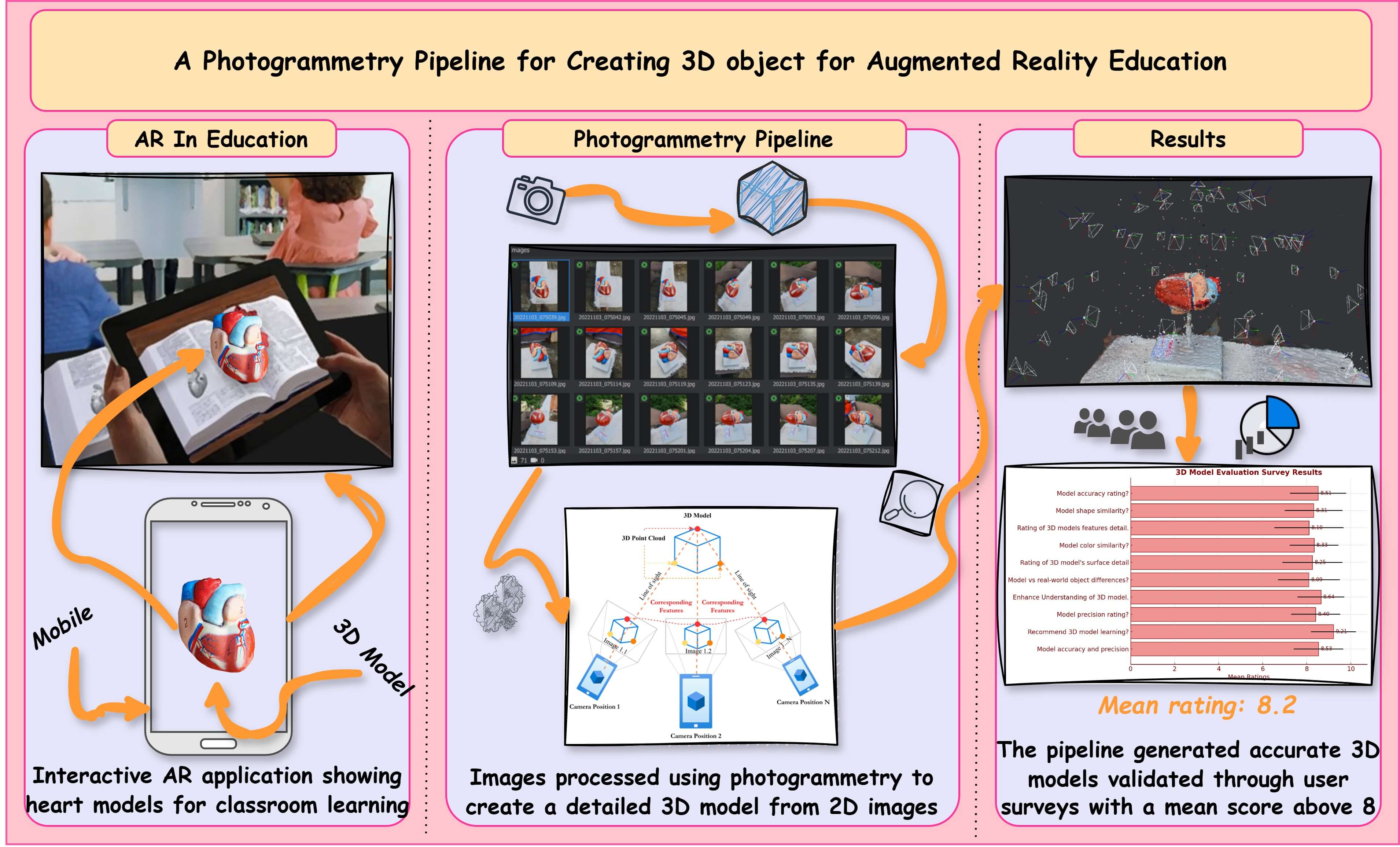
Augmented reality (AR) is an emerging dynamic technology that effectively supports education across different levels. The increased use of mobile devices has an even greater impact. As the demand for AR applications in education continues to increase, educators actively seek innovative and immersive methods to engage students in learning. However, exploring these possibilities also entails identifying and overcoming existing barriers to optimal educational integration. Concurrently, this surge in demand has prompted the identification of specific barriers, one of which is three-dimensional (3D) modeling. Creating 3D objects for augmented reality education applications can be challenging and time-consuming for the educators. To address this, we have developed a pipeline that creates realistic 3D objects from the two-dimensional (2D) photograph. Applications for augmented and virtual reality can then utilize these created 3D objects. We evaluated the proposed pipeline based on the usability of the 3D object and performance metrics. Quantitatively, with 117 respondents, the co-creation team was surveyed with open-ended questions to evaluate the precision of the 3D object created by the proposed photogrammetry pipeline. We analyzed the survey data using descriptive-analytical methods and found that the proposed pipeline produces 3D models that are positively accurate when compared to real-world objects, with an average mean score above 8. This study adds new knowledge in creating 3D objects for augmented reality applications by using the photogrammetry technique; finally, it discusses potential problems and future research directions for 3D objects in the education sector.Graphic Abstract
Keywords
In recent years, advancements in photogrammetry have revolutionized various fields by enabling the precise reconstruction of 3D objects from 2D images. This technique, rooted in computational geometry and computer vision, facilitates the creation of digital replicas of physical objects for different sectors and applications [1,2]. Photogrammetry holds tremendous promise for enhancing educational practices and methods across various disciplines in the scholastic environment. By leveraging digital imagery and sophisticated algorithms like scale-invariant feature transform (SIFT) and bundle adjustment, photogrammetry offers educators opportunities to transform traditional learning experiences into new immersive and interactive engagements. Unlike conventional teaching tools, which often rely on content in static representation, photogrammetric 3D models provide dynamic visualizations with augmented reality [3,4]. Augmented reality enhances the physical environment seamlessly, integrating with photogrammetric 3D models, which allows students to explore spatial relationships, analyze complex structures, and interact with virtual reconstructions of real-world objects in their environment [5]. Many studies state that augmented reality enhances understanding levels and promotes deeper engagement and retention of educational content.
Despite the transformative potential adaptation of photogrammetry in education, it is not without challenges. Issues such as image quality, computational requirements, and the need for specialized expertise are significant hurdles that must be addressed to equip its benefits. This research explores these challenges, evaluates current methodologies, and proposes practical solutions to enhance the integration of photogrammetry 3D models with augmented reality. This research aims to develop and validate the photogrammetric pipeline and optimize the quality of the created 3D model. The objectives encompass designing and developing an advanced photogrammetry-based pipeline to create high-quality, realistic 3D objects from 2D images captured by smartphone cameras. The primary contributions of this study concluded as follows:
• We present the optimized photogrammetry pipeline in the context of laboratory human heart reconstruction in 3D and considerations for IV-grade educational applications.
• We conduct a precision analysis and correction of the 3D models generated from the laboratory human heart images with respect to their point clouds, mesh, and textures.
• We conduct a pilot study to verify the performance and accuracy of the created 3D model.
To achieve this goal, we planned to address the following two research questions:
RQ1. How can photogrammetry pipelines improve the precision and realism of 3D models for augmented reality?
RQ2. What are the complex challenges associated with the proposed pipeline, and how can they be addressed to increase the efficiency and accuracy of the created 3D assets using photogrammetry-based pipelines?
The remaining paper is structured as follows: Section 2 discusses the previous technological workflow for reconstructing 3D models for augmented reality with photogrammetry. Section 3 describes the proposed methodology used to develop the 3D object. Sections 4 and 5 present the proposed photogrammetry pipeline. Section 6 evaluates the experimental setup, results, and discussion. Finally, Section 7 concludes the paper with future work and a summary of the key contributions.
Photogrammetry has been one of the salient methods for creating 3D objects from 2D images. This paper investigates the recent improvements in photogrammetry and its multiple uses within different areas. By examining how photogrammetry integrates with other technologies like Augmented Reality and Virtual Reality, this section provides the transformative potential of this approach for enhancing learning, visualization, and scientific research.
2.1 Integrating Photogrammetry with Augmented Reality
Andersen et al. [6] enhanced the user experience for photogrammetric 3D reconstruction by predicting covering views for efficient image capture, aiding in creating detailed 3D objects for augmented reality applications. The authors found that AR Head Mounted Display guidance improved reconstructions without unsuccessful attempts and generated views that helped capture images suitable for 3D reconstruction.
Chen et al. [7] explored the feasibility of photogrammetric techniques for creating detailed 3D meshes using Unmanned Aerial Vehicle (UAV), which enables segmentation and object extraction for virtual environments and simulations. The authors created detailed 3D meshes for augmented reality by segmenting point clouds and extracting object information crucial for virtual environments and simulations. They find the point cloud segmentation and information extraction framework proposed for part of the One World Terrain project for creating virtual environments.
Portalés et al. [8] identified that photogrammetry creates high-accuracy 3D models integrated into augmented reality, enhancing visualization and interaction in physical and virtual city environments. The authors concluded the synergy of AR and photogrammetry for 3D data visualization with low-cost outdoor 3D photo-models mobile AR applications for urban spaces. Apollonio et al. [9] analyzed the result of a photogrammetry-based workflow for accurate 3D construction of museum assets, supporting non-experts with easy-to-use methods for study, preservation, and restoration, aligning with augmented reality applications. They found this methodology combines acquisition with mobile devices and real-time rendering, and the workflow supports non-experts in museums with easy-to-use techniques.
2.2 Photogrammetry for Diverse Applications
Zhang et al. [10] outlined the steps involved in utilizing photogrammetry from UAVs to create 3D models for augmented reality mapping of rock mass discontinuities, enhancing on-site visualization, and rockfall susceptibility assessment. The authors proposed the Pro-SP template model improves edge tracking performance for AR mapping rockfall hazard visualization on actual slopes.
Rao et al. [11] proposed object-level 3D reconstruction for in-vehicle applications and monocular 3D shaping for cost-efficient 3D object creation in augmented reality and using a single-frame monocular camera setup for enhancing the in-vehicle AR applications. Titmus et al. [12] provided a description of how photogrammetry was utilized in the study to create photorealistic 3D cadaveric models, showcasing its effectiveness for generating detailed anatomical representations from actual specimens. They identified that the developed workflow for creating photorealistic 3D cadaveric models digitized eight human specimens with unique anatomical characteristics. Leménager et al. [13] reported on the findings of a study investigating the use of photogrammetry for rapid and accurate 3D reconstruction of flowers from 2D images, offering a cost-effective alternative to microCT and enabling the study of flower morphology in 3D.
2.3 Advancements in Emerging Photogrammetry Techniques
Rong et al. [14] proposed a novel framework for efficient semantic segmentation of 3D urban scenes based on orthographic images, enhancing the segmentation of Red Green Blue (RGB) images by utilizing elevation information and mining categorical features to improve local features at each pixel. Guo et al. [15] unsolved the issues in reconstructing high-fall scenes in urban environments using UAV tilt photogrammetry. It highlights the accurate reflection of topographic features in the area through DSM models constructed based on maximum prominence values, addressing issues like acquisition mismatch occlusion in high dropout scenes.
Dowajy et al. [16] proposed a comprehensive approach for automatic road segmentation in non-urban areas using shallow neural networks. By converting raw point cloud data into a regular grid, the method employs neural networks to extract road cells, refine them, and segment road points based on intensity and geometric features. The approach demonstrates high accuracy and performance, confirming its adaptability to different road environments and supporting autonomous driving applications. Li et al. [17] evaluated the precision and completeness of 3D models generated from optimized views photogrammetry in complex urban scenes. It demonstrates the potential of this method for high-quality 3D reconstruction and model updating, especially in urban areas with occlusions, showcasing improved image orientation accuracy and model quality.
Gil-Docampo et al. [18] introduced a novel method for creating 3D scale models of hard-to-reach objects using a low-cost unmanned aerial system (UAS) and Structure from Motion-Multi-View Stereo (SfM-MVS) photogrammetry. By designing a scaling tool carried by the aircraft to determine the object’s actual size, the procedure achieves good dimensional accuracy in the 3D model. The results demonstrate an error of less than 1 mm in almost 90% of the point cloud, validating the effectiveness of the new approach. Kubišta et al. [19] discussed creating animated digital replicas of historical clothing by analyzing conserved ring armor and building models composed of individual rings. Advances in textile simulation algorithms are highlighted, focusing on rich texture details in digital models. The quality of UV unwrapping for mapping 3D model surfaces onto 2D images is emphasized, with methods involving geometric projection of seams marked on clothing photographs onto 3D models. The study showcases innovative techniques for creating detailed digital replicas of historical clothing.
The reviewed literature demonstrates how photogrammetry can be used in diverse applications, from creating detailed 3D models for AR displays [6,8] to making precise anatomical models to teach [12]. Advancements in photogrammetry techniques address challenges like efficient image capture and reconstructing tall structures [15]. However, there is a gap in the research on optimizing photogrammetry for teaching in an augmented reality environment. This study aims to fill this gap by examining how to make 3D models with photogrammetry to use in AR applications for educational purposes. We will focus on creating high-quality 3D models using image analysis techniques to improve visual details; additionally, we will employ advanced reconstruction methods to ensure accurate 3D reconstruction to use in our future research for elementary school science textbooks.
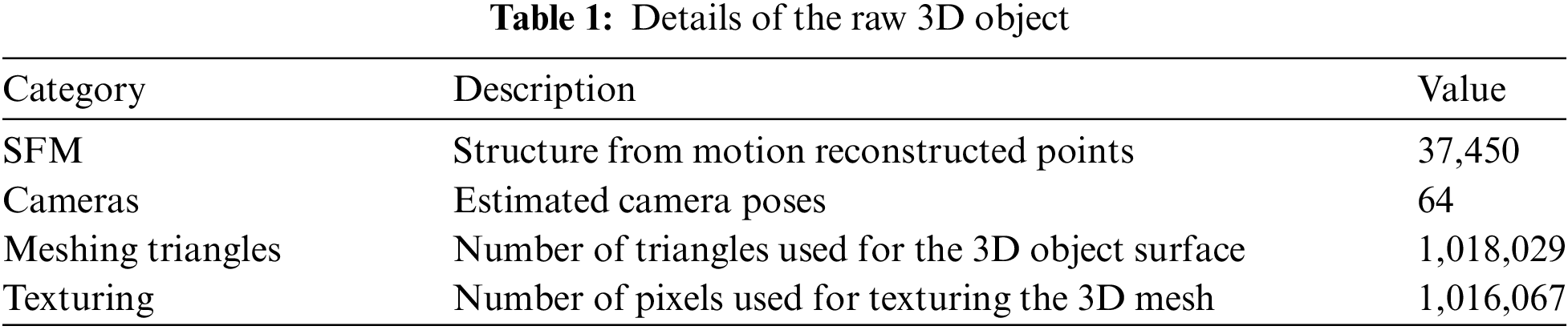
Following the background from the previous section, this research presents an innovative approach to creating 3D objects using the photogrammetry pipeline illustrated in Fig. 1. The proposed methodology comprises several fundamental phases, starting with data collection through the utilization of a mobile camera for photographing a laboratory human heart. Techniques such as feature detection, motion structuring, depth mapping, meshing, and texturing are incorporated into the proposed pipeline. The proposed system enables the conversion of physical objects into 3D models, thereby transforming them into valuable assets for various applications. Two major components of this research are data acquisition and 3D reconstruction using photogrammetry.
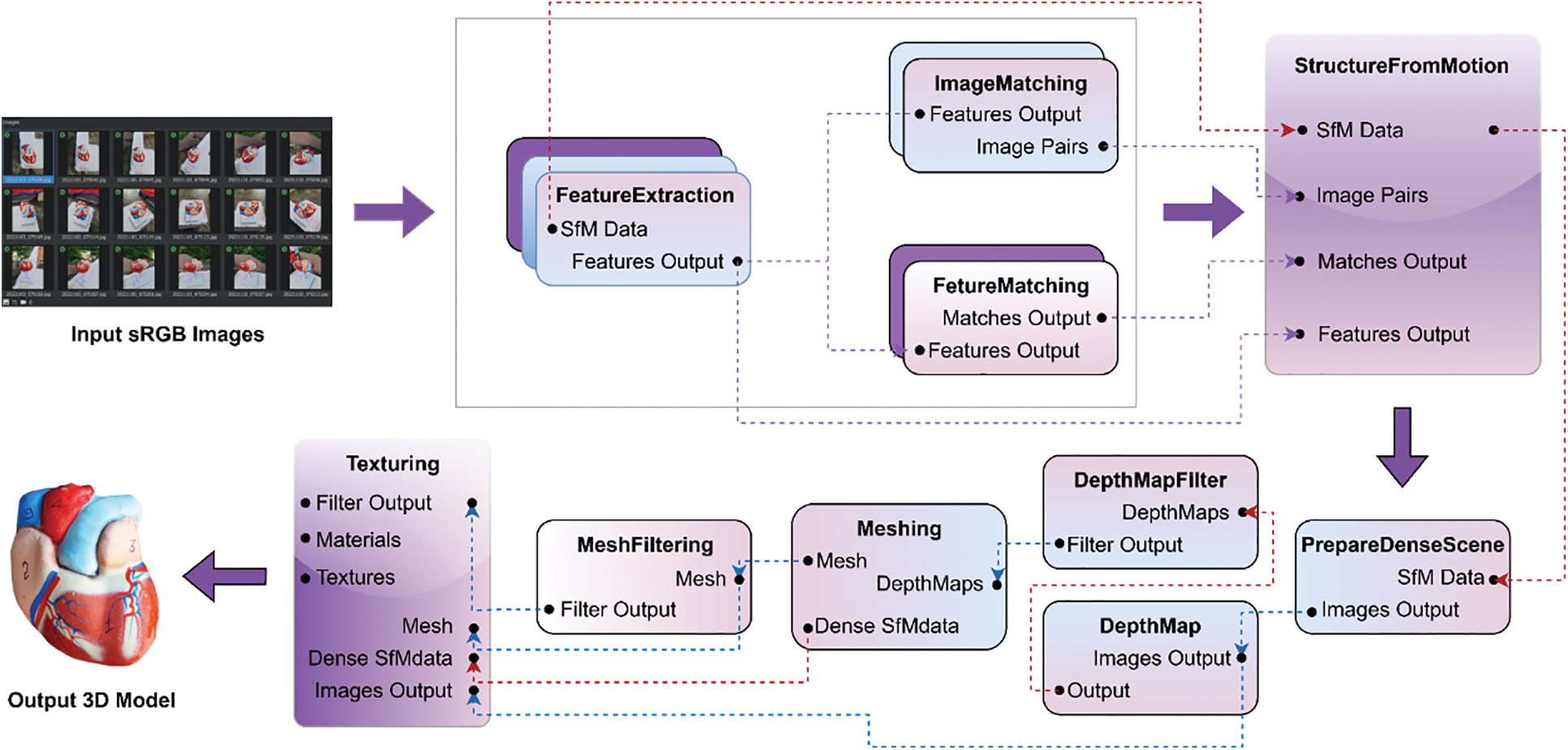
Figure 1: Proposed photogrammetry pipeline for 3D object reconstruction
There are various camera setups available when taking photographs of real objects. Single-camera [20], multiple-camera [21], and handheld-camera [22] setups are the most popular. Single cameras can move and adjust to collect photographs from different angles. Furthermore, having a single camera avoids time-consuming and synchronizing difficulties between other cameras used in multiple camera setups. Photographic data for the 20 cm × 10 cm human heart will be captured using a mobile camera. To achieve the best possible image quality, we take the data in daylight with natural lighting and set the ISO, aperture, and shutter speed to a fixed value. It is important to capture several pictures of an object from various angles to guarantee the total inclusion of its surface. This is a crucial stage in creating a realistic 3D model of the same object, as it provides the foundation for the subsequent steps. Once the photographs of the object have been obtained, they are incorporated into the framework and processed through the pipeline illustrated in Fig. 1.
As the framework was being loaded with each captured image shown in Fig. 2, Reconstruction [23] requires a series of sequential phases. The first three phases, feature extraction, feature matching, and image matching, are computationally less intensive. However, the remaining phases, such as structure from motion to texturing, require significant computational power to process the data. To optimize the performance, we divide the process into two stages: Image Analysis Techniques and Advanced Techniques for 3D Model Reconstruction. The Image Analysis Techniques identify features in the images, and the Advanced Techniques for the 3D Model Reconstruction stage create the 3D model using the identified features.
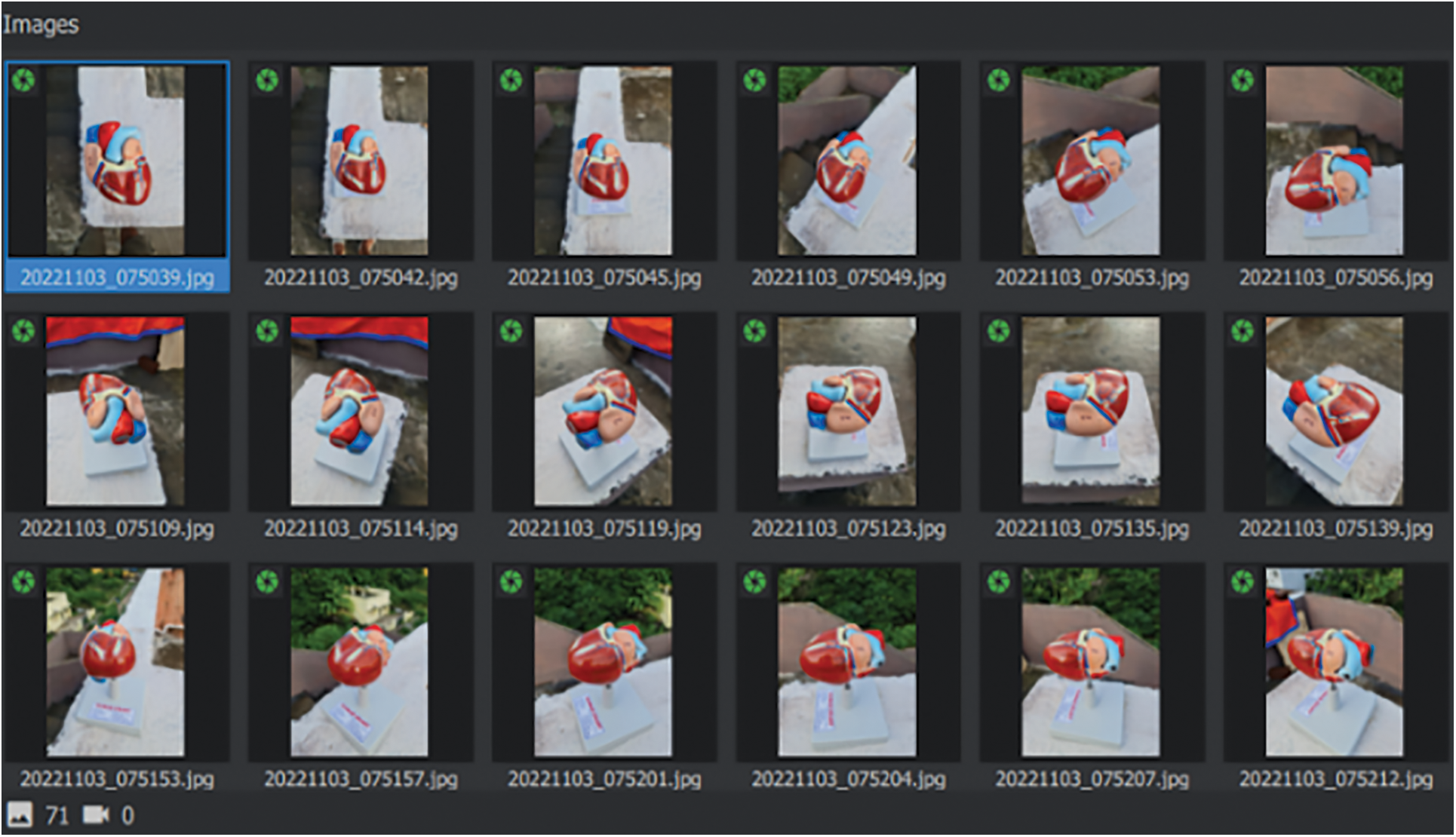
Figure 2: Images loaded into the framework
Feature extraction [24] dentifies distinctive and stable features in each input image, such as corners or edges shown in Fig. 3. This is used to match corresponding features in other images. These features were identified using the SIFT feature detection algorithm. The left panel in Fig. 3 shows the initial step of feature extraction, where key points are identified from a single image using the SIFT algorithm. These key points are visually represented by yellow markers scattered across the image, denoting areas of high distinctiveness and repeatability. The SIFT algorithm identifies these keypoints by convolving the image with a Gaussian function (1) filter at different scales to create a scale space. Then keypoints are detected by finding local extrema in the difference-of-Gaussian (2) scale space.
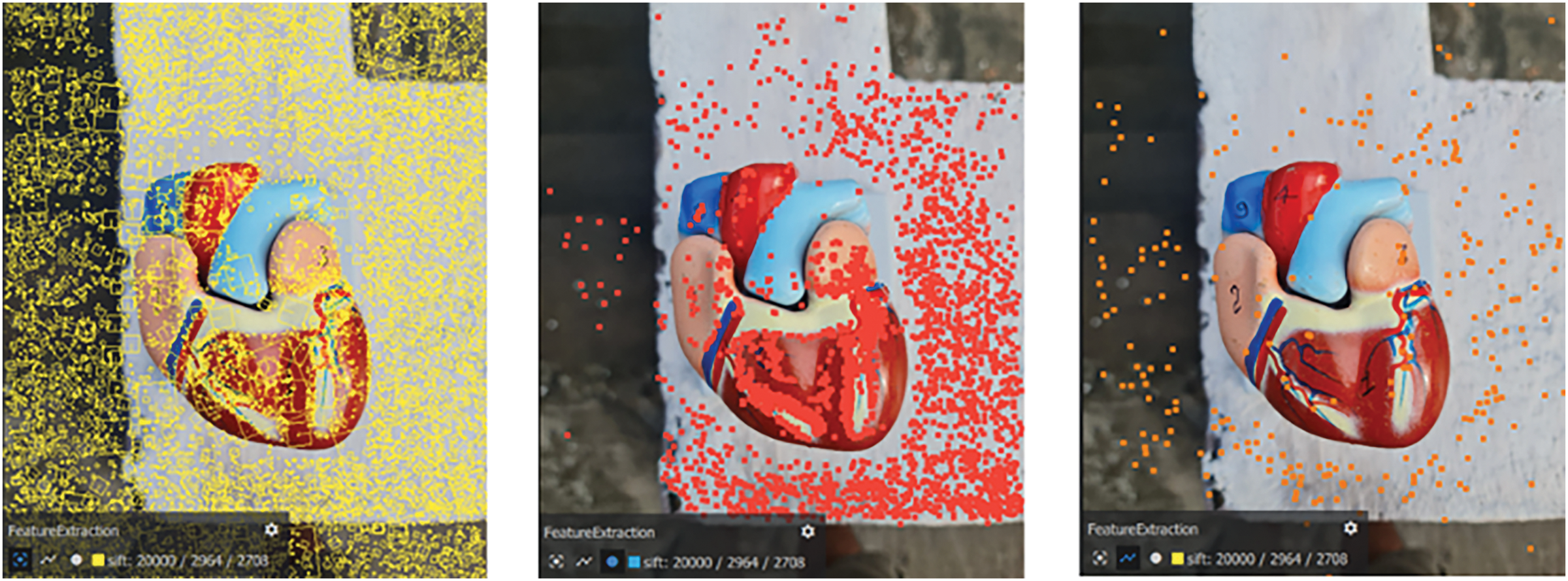
Figure 3: On the left, is the feature key points extracted from an image, represented by yellow markers (Feature extraction). The landmarks extracted from the same photo, represented by a red marker (Feature matching) in the center. On the right, the 3D point cloud created by matching the feature key points from multiple images, represented by orange markers (Image matching)
where
where
Feature matching [25] is the process of identifying corresponding features between pairs of images. In the center panel from Fig. 3, the extracted key points are refined into landmarks, represented by red markers. This refinement is achieved through a feature matching process, where only the most relevant and accurately matched keypoints with associated feature descriptors (3). We use these feature descriptors to compare features between images, capturing the local appearance and geometry of the features. SIFT can identify features invariant to changes in scale, rotation, and lighting, making it suitable for matching features between images taken from different viewpoints and under different lighting conditions. Once the feature matching is complete, we use the correspondence between keypoints in various images to estimate the relative camera positions and orientations that capture the same object or scene from different viewpoints. This forms the basis for the next step in the proposed photogrammetry pipeline, which is image matching. We compute the Euclidean distance between feature descriptors to match features between pairs of images. Let us say we have two feature descriptors represented as vectors. The formula provides the Euclidean distance between these vectors.
where
Image matching [26] is adjusting different images of a scene or item by assessing their overall camera positions and directions. The right panel visualizes the creation of a 3D point cloud, represented by orange markers. This point cloud is generated by matching the feature key points across multiple images, effectively reconstructing the 3D structure of the object from various perspectives. The orange markers indicate the spatial distribution of these points in a 3D space, demonstrating how the combined data from multiple images coalesce into a coherent 3D model. This is done by utilizing the correspondences between the matched features (keypoints) recognized in the feature-matching step. The thought behind image matching is to track down the change (rotation and interpretation) that maps one picture onto another. Image matching (4) includes assessing the change matrix T between sets of pictures utilizing correspondence between matched features.
The transformation matrix
where the rotation matrix’s elements are
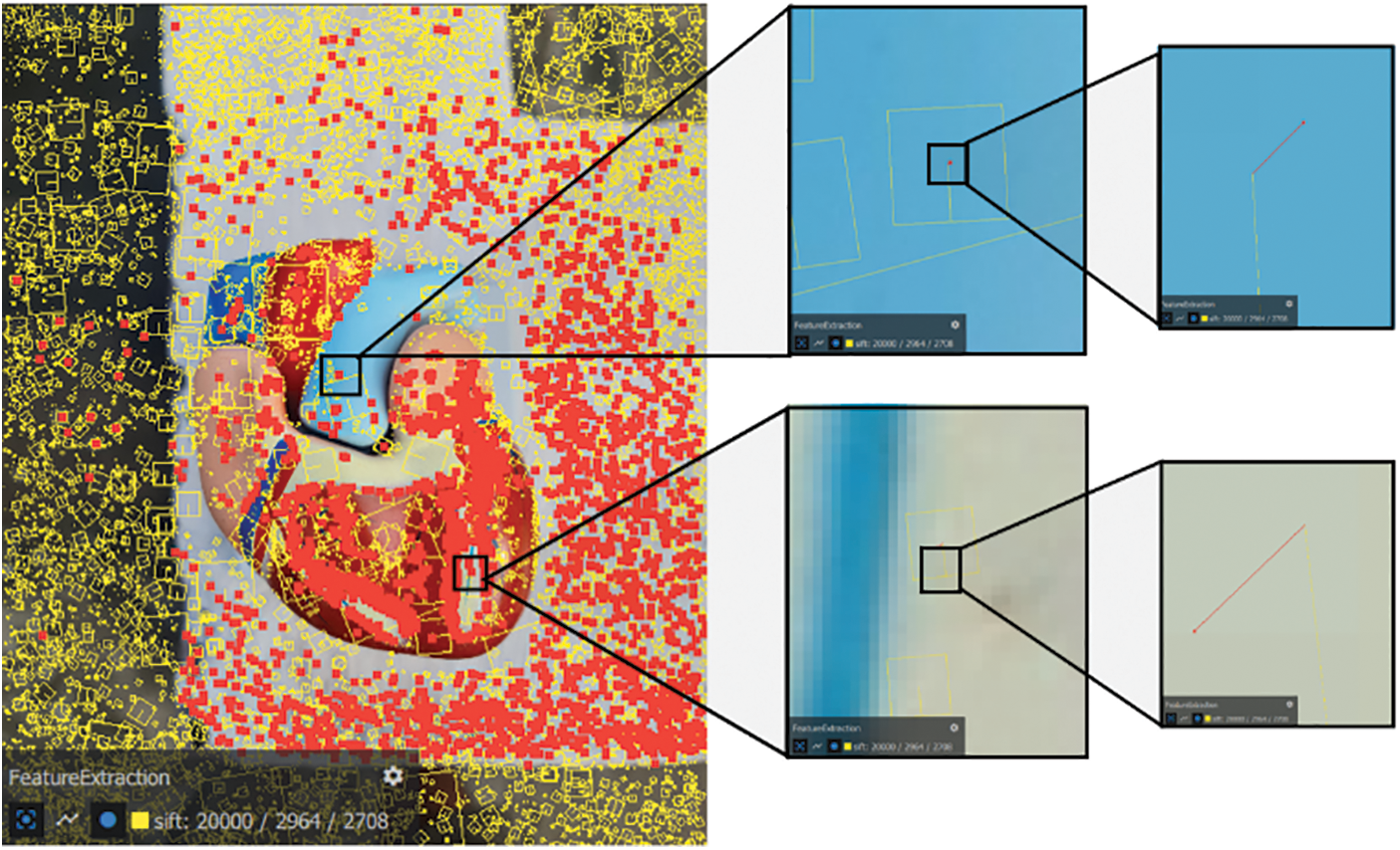
Figure 4: Position of the 2D feature (yellow box), corresponding projection of the 3D landmark (red point), and the line segment (red) in between is the reprojection error
Fig. 4 illustrates the process of feature extraction from a 3D model, highlighting how distinct features are identified and their relationships to the surrounding structures. This figure is composed of a primary image on the left, showing the entire model with numerous feature points overlaid, and three zoomed-in views on the right, each magnifying specific areas of interest on the model. The main image displays a 3D model with a multitude of feature points highlighted in red and yellow. These points represent key areas detected by feature extraction algorithms (such as SIFT, as indicated in the bottom-left corner). The overlay of these features on the model provides a comprehensive view of how the algorithm identifies significant points across the entire object. The color coding (yellow and red) may indicate different categories or thresholds of feature significance, allowing for differentiation between highly prominent and less prominent features. The dense clustering of feature points in certain regions corresponds to areas with greater texture or detail, which are critical for accurate 3D reconstruction and representation. The top zoomed-in view focuses on a specific section of the model, likely corresponding to a distinct color or surface feature. This magnification reveals how the feature points are distributed within this local area, showcasing the precision of the extraction process in identifying minute details. The view provides an in-depth look at the alignment and spacing of the points, which are crucial for maintaining the fidelity of the 3D structure when viewed or interacted with in an immersive environment. The bottom zoom-in captures another area of the model, providing a close-up of a boundary region between two different surface textures or colors. This view highlights the feature extraction’s ability to discern between contrasting surfaces, which is important for accurately representing boundaries and transitions in the 3D model.
5 Advanced Techniques for 3D Reconstruction
Structure from Motion (SfM) [27] is a method used to estimate the 3D design of a scene or object from a bunch of 2D pictures. The objective of SfM is to estimate the camera positions and directions for each picture and the 3D directions of the places in the scene that compare to features in the images. Fig. 5 represents the semantic view of SfM. The process of SfM includes a few stages:
• Key features are extracted from each image by SIFT, depicted by the descriptors.
• The corresponding features of two images are used to match features that are similar to one another.
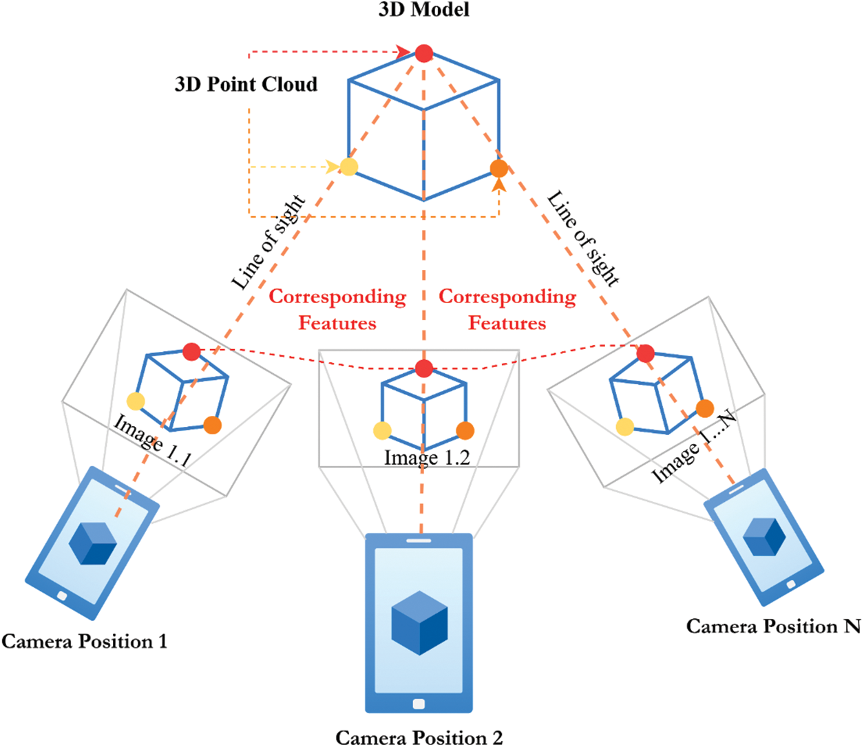
Figure 5: Structure from motion schematic diagram
The general positions and directions of the cameras for each picture are evaluated considering the correspondence between the features in each picture. The 3D coordinates of the features are estimated based on the camera poses and the correspondence between the features in each image. Bundle adjustment is a crucial step in SfM, improving the accuracy of the estimated camera poses and 3D point cloud. The process involves optimizing a cost function that balances the reprojection error and the regularization term, which penalizes deviations from the initial estimates. In a RANSAC framework [28], Resectioning is based on a perspective-n-point algorithm (PnP) [29], which finds the camera pose most accurately and validates the feature associations. To enhance the camera’s positional accuracy, a non-linear adjustment technique is applied to each individual camera. This results in new camera positions and causes some points to be visible in multiple images, allowing for their 3D position to be determined through triangulation. After all extrinsic and intrinsic camera parameters, all 3D point positions are refined by bundle adjustment. Eq. (5) shows the mathematical model for bundle adjustment.
where
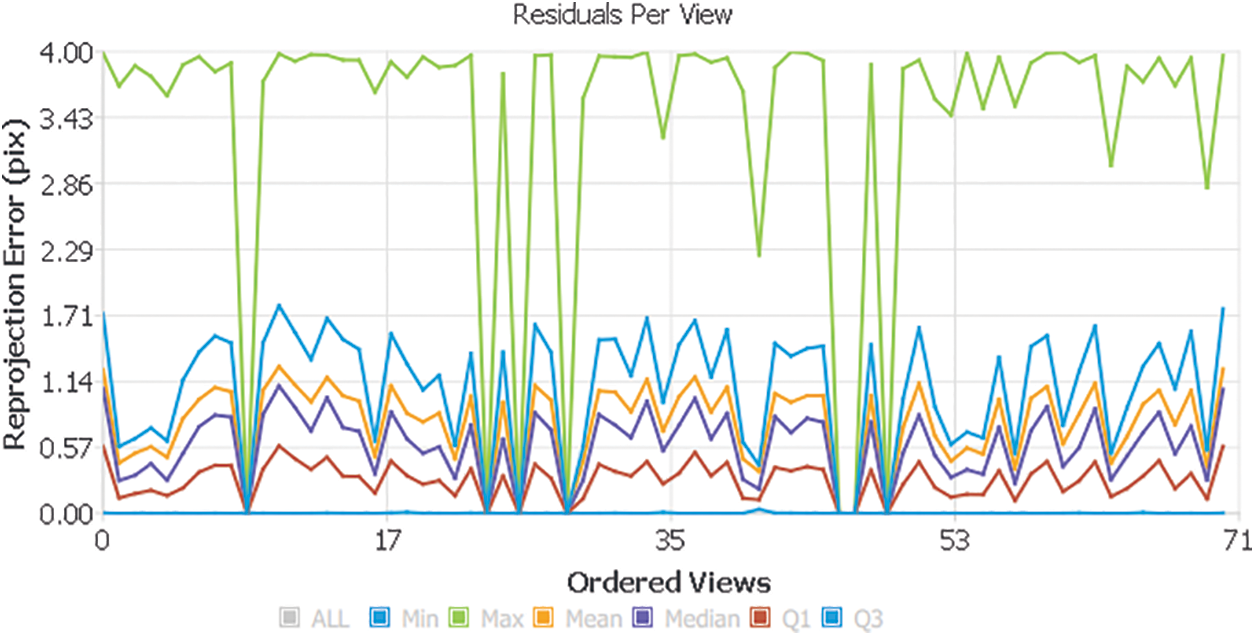
Figure 6: Reprojection error
A higher “observation length per view” shown in Fig. 7 indicates that the corresponding image contained more features useful for constructing the 3D object.
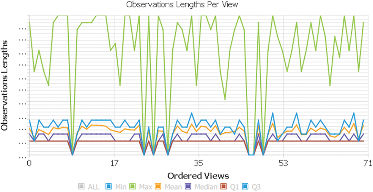
Figure 7: Observation length
We analyzed the “Landmarks Per View” visualization in Fig. 8 to determine the number of feature points identified in each of the 71 images used for reconstruction. Landmarks are keypoints that track across images to build the 3D model. A higher number of landmarks in an image generally indicates more potential features for building the 3D model. By finding new points through triangulation, more potential viewpoints are obtained for further analysis. The process continues in this manner, adding cameras and triangulating new 2D features into 3D Cloud points with landmarks while removing invalidated 3D Cloud points and repeating until it can no longer localize new views.

Figure 8: Number of landmarks
Once the camera poses and 3D point have been estimated, the 3D structure of the scene or object can be visualized (shown in Fig. 9) or used for further analysis.
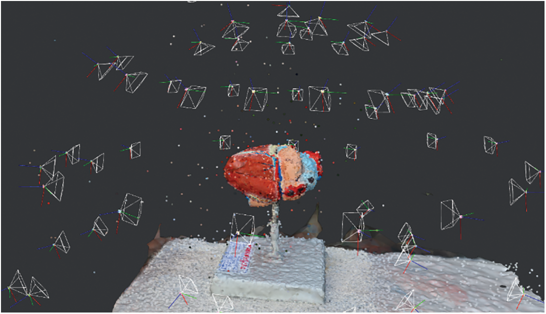
Figure 9: Output from structure from motion
To increase the density of the point cloud generated in the previous steps, it is necessary to calculate depth estimates for each pixel in every image using SfM techniques, which involve triangulating correspondences between features in the images to estimate the depth of each pixel. Afterwards, we can compute the depth of each pixel by projecting the 3D points onto the image plane, as illustrated in (6):
where
Following the preparation of a dense scene [31] in 3D reconstruction, depth maps for each input image are generated to indicate the distance from the camera to each point in the scene. Depth maps generated from input photos are critical in 3D reconstruction because they allow for accurately positioning 3D points. The reconstructed 3D model can be built with great precision by estimating the distance to each point in the picture. To construct depth maps, computer vision algorithms assess each input image and estimate the distance between the camera and each point in the scene. To calculate the depth maps for each input image, an optimization process is performed using the following (7):
where
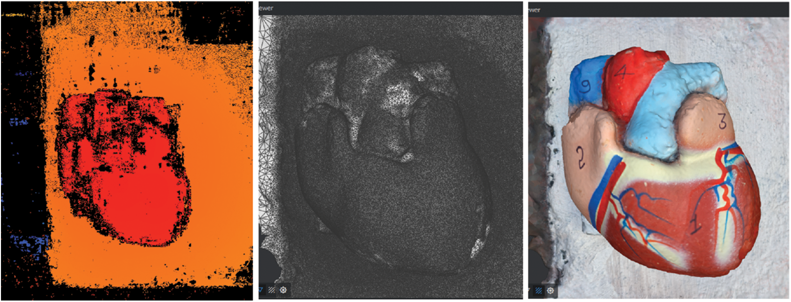
Figure 10: Left image represents the DepthMap, center image represents the mesh, and right image represents the textures
After building a dense scene in 3D reproduction, depth maps used for portraying the distance from the camera position to each point in the scene are created for each image. These depth maps may contain noise and artifacts, bringing about botches in the last 3D remaking. To resolve this issue, depth map filtering (8) is used in the next step. One standard strategy is to utilize a filtering noise that substitutes every pixel’s depth value with a weighted normal of the depth value of its neighbors.
where
Creating a 3D mesh from a dense point cloud and filtered depth maps involves two main steps: surface reconstruction and mesh generation [32]. Let
where
where g is a function that takes the surface
where
The strategy of 3D recreation includes adding realistic colors and textures to an object’s surface. Making a 3D object look more real involves projecting a 2D image or texture onto its surface [33,34]. There are different cycles associated with the texture mapping process. Let O be a 3D object represented as a mesh section M comprising of vertices, edges, and faces. And T to be a 2D surface picture addressed as a matrix of pixels with width W and level H. The process of texture mapping involves the following steps:
i. Unwrapping: The 3D mesh
ii. Applying the texture: The 2D texture (13)
The texture coordinates for each pixel in the face can then be obtained by interpolating the values at the vertices (17) and (18):
where
The color of the pixel can then be obtained by evaluating the texture (19) function
iv. Displaying the textured object: The colored faces are displayed on the surface of the 3D object, creating the appearance of a realistic, textured surface shown in Fig. 10 right image.
In Fig. 10, a range of illustrations are shown that detail the processes involved in turning imaging data into a 3D model to offer better instructional materials for primary school students within immersive learning settings. It contains three images that represent the depth map, mesh, and textured model of a biological structure. On the left side of this figure is shown a depth map that encodes 3D objects’ depth information using shading or color intensity in 2D only. Depending on how far or near they are from the scanning source, surfaces close to the depth scanner will appear warm, while those located farther away will appear cool. Even though this 2D feature captures essential depth information, it is not meant to convey a complete 3D view. Instead, it serves as a preliminary step towards building the subsequent 3D models. In our learning context, this representation, therefore, helps students understand depth perception in simplified terms appropriate for learners. The central picture brings forth the mesh, which is one of the key intermediate geometries of 3D maps that are restructured into its vertices, edges, and faces formed by the depth map. This mesh comprises the object’s skeleton in a geometric sense; its spatial relationships and shape are represented more adequately than 2D images. The mesh serves as an important source of understanding for complex structures because it provides a concrete 3D form that captures their overall shape and construction. In this representation, students can investigate and manipulate 3-dimensional figures to better comprehend them in space and improve their engagement with the contents. The image on the right shows the Textured Model applied to a 3D mesh where detailed textures are added onto it, giving rise to an object that can be described as duly realistic as well as visually complex. At this final phase, surface details such as colors, labels, or patterns come into play, resulting in a 3D model.
As part of this experimental work is shown in Table 2, we used Samsung Galaxy Note 20 Ultra (SM-N986B) smartphones to capture physical objects. To ensure all the images are in the same lighting, as we said earlier in Section 3, we used the pro (manual) mode in the camera application to set up the fixed aperture size, shutter speed, and ISO to capture multiple photos. The following are the camera specifications: 108 Mega Pixel (it uses 3 × 3 pixel binning to produce a final image of 12 Mega Pixel). Samsung ISOCELL Bright HM1 Sensor, 1/1.33” image sensor size, aperture f/1.8, a focal length of 26 mm with 79° field of view, laser and phase detection autofocus, and optical image stabilization (OIS) were used to capture the sRGB images. Photos taken with a 12 Mega Pixel camera have a resolution of 3000 × 4000 pixels (0.8 m pixel size), an ISO of 50, and shutter speeds ranging from 1/368 to 1/908 s at f1.8 stationary objects with 7.0 mm. By this, we can avoid the lighting issues, and all captured images are in the same exposure level with geotagging and stored in 4:3:0 subsampling of.jpeg format and an Asus ROG Strix G531GT laptop with an Intel(R) Core (TM) i5-9300 CPU @ 4 GHz, 16 GB DDR4 RAM, and a 4 GB Nvidia GeForce GTX 1650 Graphics Card to process the captured data. We utilized Meshroom and Blender open-source software for the 3D object creation with our tweaked version of computer vision algorithms. The first stage is for identifying features in an image; it takes 20 min and uses the full computational power of the CPU at 3.42 GHz, bringing about a temperature of 74°C and a fan speed of 4800 RPM. The subsequent stage is making the 3D model, which executes for 57 min and uses 98% of the GPU, 4 GB Nvidia GTX, bringing about a temperature of 67°C and a fan speed of 5100 RPM. This stage is known to be computationally serious, and the outcomes show that our experimental setup handled the computational demands. The results show that our proposed pipeline is fit for handling the computational requests of the photogrammetry framework and can be successfully utilized to make excellent 3D models for education in our future work as well as other 3D objects.
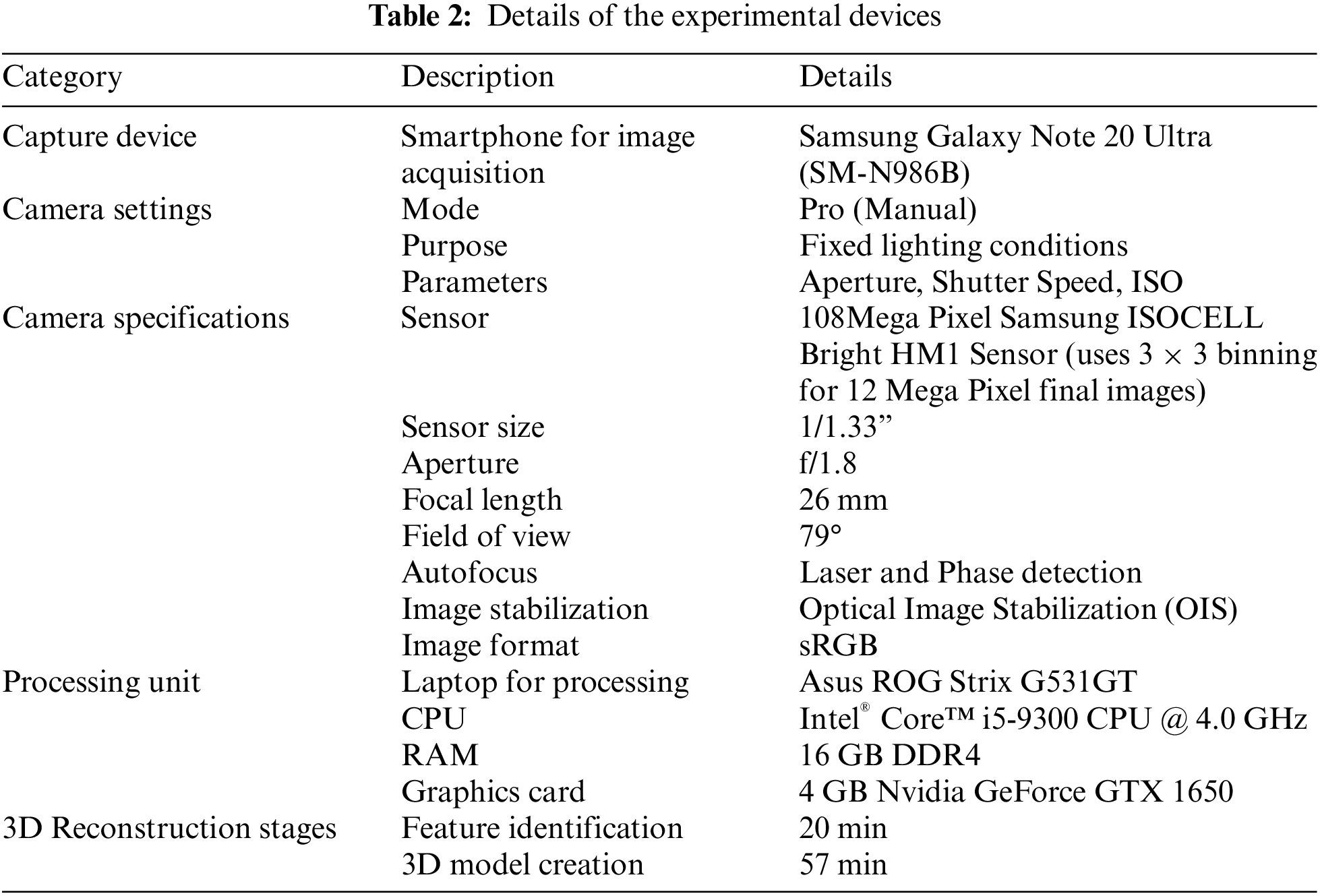
The implementation of this proposed pipeline addresses the potential barriers of time and cost in creating detailed 3D models. This is demonstrated by the fact that our method not only maintains model quality but also significantly cuts down on the associated expenses and time requirements shown in Table 2, we provide a viable solution for those seeking cost-effective alternatives to traditional methods.
The photogrammetry framework produces a model in the .obj file format, and the meshes are exported with one million triangles. These triangles do not add meaningful details but instead generate unnecessary or unwanted scan surfaces and noise from the entire data set. Even though numerous frameworks can handle high-density 3D models effectively, the handling time for the 3D model might fluctuate based on the system configuration with respect to the triangles. It is important to remove noise or undesirable output surfaces as a basic move toward the optimizing process, as it can essentially work on the final 3D object’s visual quality and performance. As per our needs, only the heart portion from the reconstructed 3D model is required, but the output 3D model, which includes the entire structure, including the base, stand, holder, and heart, is depicted in the left image of Fig. 11. Table 3 shows that the created 3D model is the final type of .obj with a file size of 70.6 megabytes in the output folder. We import the created 3D model into Blender to remove the undesirable surfaces and noise.
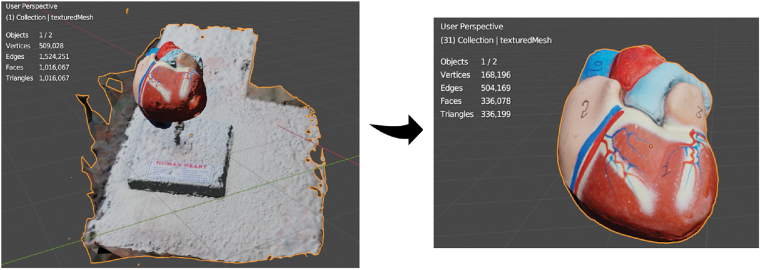
Figure 11: Final 3D model from the original 3D object
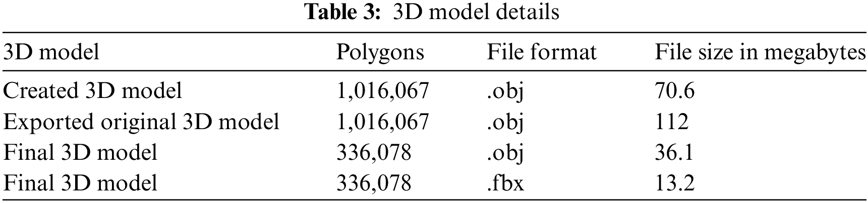
The imported 3D model has 509,028 vertices, 1,524,251 edges, 1,016,067 faces, 1,016,067 triangles, and a file size of 112 megabytes, which requires more processing time and power to compute. After removing the unnecessary scanned surface from the original 3D model, we did additional sculpting and modeling to the remaining scanned area to get a realistic 3D object (Fig. 11 right image). We obtained the final required “3D Asset” heart part from the original whole 3D object in .obj and .fbx file formats. The final 3D heart asset contains 168,196 vertices, 504,169 edges, 336,078 faces, 336,199 triangles, and a file size of 36.1 megabytes. Education, medical research, visualization, and animation can all benefit from the highly accurate and detailed representation of a heart in the final 3D heart asset shown in Fig. 11. Furthermore, it can be used in real-time rendering, virtual reality, augmented reality, and mixed reality educational applications.
6.3 Discussion on Research Questions
RQ1. How might photogrammetry-based AR pipelines work on the precision and realism of 3D models?
By investigating and implementing different strategies, like Feature Extraction, Image Matching, Feature Matching, Structure from Motion, Prepare Dense Scene, Depth Map, Depth Map Filter, Meshing, Mesh Filtering, and Texturing.
RQ2. What are the complex difficulties related to the proposed pipeline, and how might they be addressed to build the effectiveness and accuracy of 3D assets utilizing photogrammetry-based pipelines?
We found a few complex issues with the proposed pipeline for delivering 3D objects utilizing photogrammetry-based pipelines. Some of the challenges include meshing, feature extraction, image matching, and camera calibration. Camera calibration, necessary for accurate 3D modeling, is quite possibly one of the most difficult challenges. Measurement inaccuracies and model distortions can result from inaccurate calibration. To resolve this issue, we utilized manual camera calibration techniques like fixed aperture, shutter speed, and ISO, which worked on precision and efficiency. Feature extraction and matching are also critical pipeline components. To produce a 3D model, these techniques entail finding and matching typical features in many photos. However, feature extraction might be harrowing in photos with poor contrast, noise, or occlusion. We captured the photographs using a manual camera arrangement to avoid noise or occlusions to overcome this issue. Another critical phase in the pipeline is meshing, which includes creating a 3D mesh from the point cloud generated by the photogrammetry workflow. This procedure is time-consuming and computationally demanding. We optimize the meshing process to increase the efficiency of this operation by minimizing the number of triangles necessary to represent the 3D object.
In addition to the challenges of 3D modeling, successful integration of augmented reality in education also depends on factors such as hardware availability and cost. To address hardware concerns, the 3D models developed through our photogrammetry pipeline are optimized for compatibility with a range of modern smartphones, making the technology accessible to a wider audience. This reduces the reliance on high-end equipment and helps alleviate cost-related barriers.
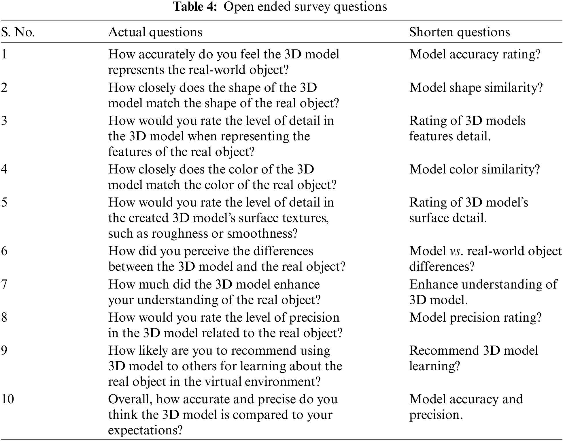
The accuracy and precision of a 3D model created from 2D photos using the proposed photogrammetry pipeline were explored. The study included a sample size of 117 respondents, comprising 7 (male) professional 3D designers and 110 (50 female, 60 male) students. While this sample size was deemed appropriate for the initial phase of this research. Future studies will involve a larger and more diverse participant pool, including educators from various educational levels and a broader range of students. By expanding the sample size and demographic diversity, we aim to ensure that our findings are more reflective of the broader population, thus increasing the reliability and applicability of the results to different educational contexts. To compare the real-world physical object and the created 3D model, 117 respondents were asked to score open-ended questions (Table 4) using the Likert scale method.
The data was analyzed using descriptive statistics, and the results show that most respondents assessed the 3D model’s correctness and precision as positive and good. Furthermore, the level of detail and color depiction were rated as satisfactory. These findings positively imply from the respondents that the proposed pipeline can be a beneficial and practical approach for producing 3D models with high accuracy and precision from 2D photos. Descriptive analysis was used to analyze the data, and the results are shown (Table 5) in Fig. 12. The statistical analysis of the 3D model evaluation reveals various insights into the consistency and reliability of the models. The model accuracy rating received a mean score of 8.51 with a standard deviation of 1.277 and a variance of 1.631, indicating a generally high level of agreement among respondents, though with some variability. Similarly, the rating for model shape similarity averaged 8.31, with a standard deviation of 1.310 and a variance of 1.715, reflecting a generally favorable view but with noticeable variation in responses. The assessment of 3D model feature detail had a mean score of 8.10, accompanied by a higher standard deviation of 1.572 and a variance of 2.472, suggesting a broader range of opinions on the detail provided by the models. For model color similarity, the mean rating was 8.33, with a standard deviation of 1.106 and a variance of 1.224, indicating a consistent but slightly varied perception of color accuracy.
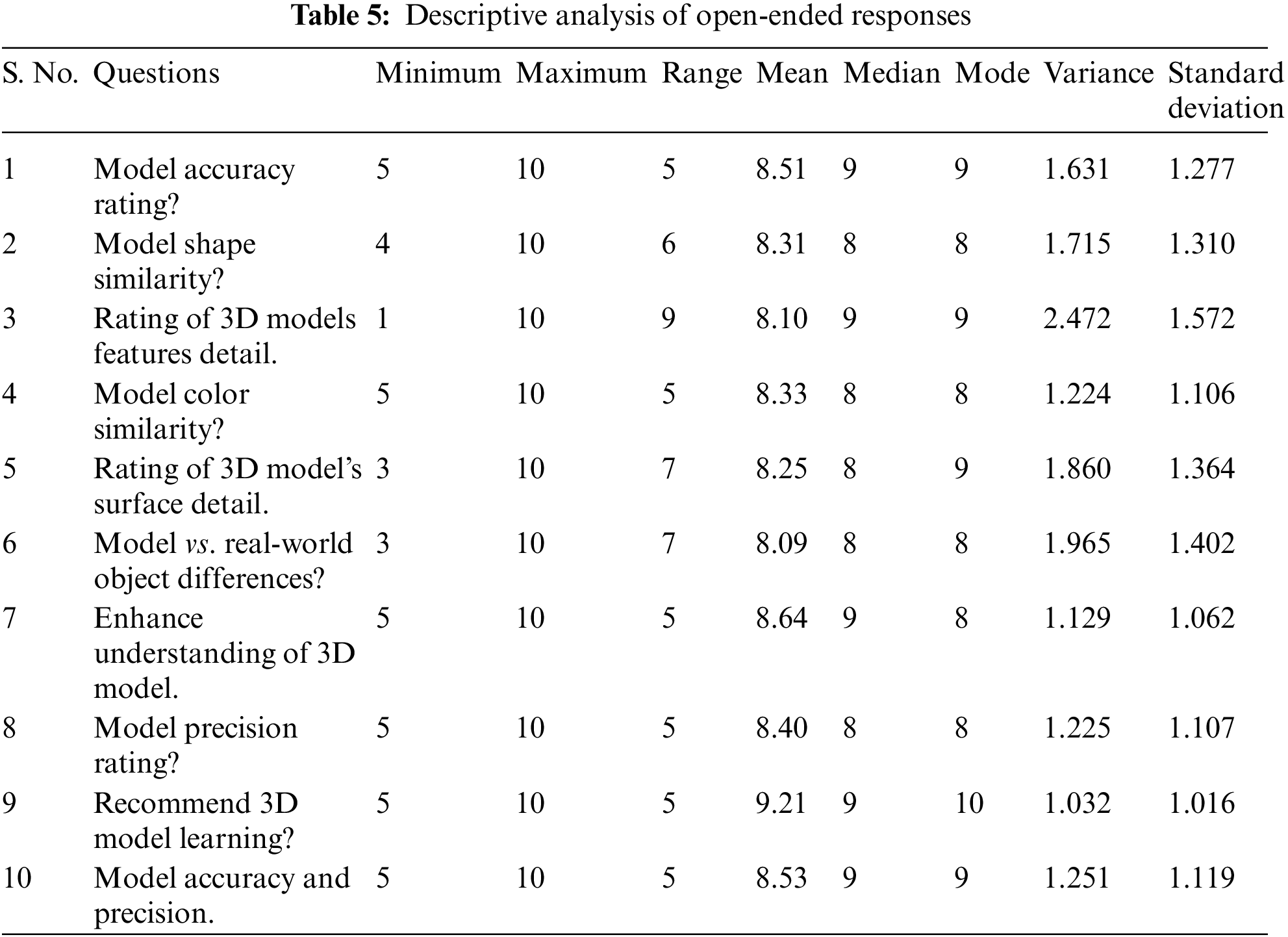

Figure 12: Overview of the survey analysis
The rating of the 3D model’s surface detail averaged 8.25, with a standard deviation of 1.364 and a variance of 1.860, showing moderate variability in how surface details were perceived. Differences between the model and real-world objects were rated with a mean of 8.09, a standard deviation of 1.402, and a variance of 1.965, pointing to a wider range of opinions regarding the model’s fidelity to real-world objects.
The enhancement of understanding provided by the 3D model received the highest mean score of 8.64, with a relatively low standard deviation of 1.062 and a variance of 1.129, indicating strong agreement on the model’s educational value with minimal variability. The precision of the model was rated with a mean of 8.40, a standard deviation of 1.107, and a variance of 1.225, suggesting general agreement on the model’s precision but with moderate variability.
The recommendation of the 3D model for learning purposes achieved the highest mean score of 9.21, supported by a standard deviation of 1.016 and a variance of 1.032, reflecting a high level of agreement with minimal variability. Lastly, the combined assessment of model accuracy and precision had a mean score of 8.53, with a standard deviation of 1.119 and a variance of 1.251, showing overall positive feedback but with some variation in responses. While no significant outliers were observed, responses with extreme values in questions regarding model feature detail and real-world object differences were noted, although they did not substantially affect the overall findings.
The discoveries shown in Fig. 12 show that the proposed photogrammetry pipeline was highly effective in creating a 3D model that precisely and definitively depicted this real-world object. Furthermore, the members strongly suggested using 3D models in school to learn concepts in virtual environments by incorporating them into the AR mobile application.
This study has successfully established a photogrammetry-based pipeline for reconstructing realistic 3D objects from 2D photographs, which can be utilized to revolutionize the field of augmented, virtual, and mixed-reality applications. This study significantly contributes to educators’ ability to create their own 3D content without extensive 3D modeling expertise. The survey evaluation confirmed the pipeline’s effectiveness. The user study (n = 177) shows that the 3D models developed with this pipeline were exact and got a positive appreciation for their precision, detail, and overall quality of the pipeline and the positive user perception of the resulting 3D object. In addition to this, the cocreation team’s feedback indicates the high degree of accuracy in the created 3D object with an average mean score exceeding 8 (on a 10-point scale).
Though the findings of this research are encouraging, it is important to recognize several significant limitations. First, the effectiveness of a photogrammetric pipeline depends upon capturing pictures at optimal lighting conditions, which may be difficult in poor regions. Also, the current framework is meant to create static 3D models with little interactivity. Nevertheless, there is a wide range of future applications of these 3D objects in education. In the future, we will add machine learning and computer vision, as well as interactive features such as animations and physics simulations, into this technology so that it becomes a more engaging and immersive augmented reality experience. This would allow students to understand better the topics from a real-world perspective; therefore, future studies will focus on assessing how much these photogrammetry-inspired 3D models impact student learning outcomes. While we intend to include these interactive features in our future work, this study does not explore the challenges of their integration. Educators can construct high-quality, immersive instructional experiences from the photographs of an object that were previously difficult and time-consuming, even for skilled people. The result of this study reveals that this can be achieved by using the capabilities of photogrammetry-based pipelines. Moving to the future, upgrading the asset’s capabilities to improve its responsiveness in real-time circumstances with seamless integration of the pipeline and its outputs with existing education platforms by incorporating machine learning and computer vision approaches with animations and physics simulations. In the current study, we primarily utilized open-ended questions to gather qualitative feedback on the precision and usability of the 3D models. While this approach provided valuable insights, future research will incorporate quantitative evaluation methods, such as precision, recall, and F-score metrics, alongside automated error measurement techniques. These methods will provide a more objective and comprehensive evaluation of the 3D models’ accuracy, allowing us to better validate the efficacy of the proposed photogrammetry pipeline.
Acknowledgement: None.
Funding Statement: The authors received no specific funding for this study.
Author Contributions: The authors confirm contribution to the paper as follows: study conception and design: Uma Mohan; data collection, analysis and interpretation of results, draft manuscript preparation: Kaviyaraj Ravichandran. All authors reviewed the results and approved the final version of the manuscript.
Availability of Data and Materials: The created 3D objects and the dataset used to generate them will be made available upon request to the corresponding authors.
Ethics Approval: This study was conducted using an anonymous online survey, collecting only basic demographic information such as age and gender, no personally identifiable information including participants’ names, was collected to ensure full anonymity. This study did not involve any medical or psychological research on human subjects and was therefore exempt from ethical review.
Conflicts of Interest: The authors declare no conflicts of interest to report regarding the present study.
References
1. Wang X, Xiang H, Niu W, Mao Z, Huang X, Zhang F. Oblique photogrammetry supporting procedural tree modeling in urban areas. ISPRS J Photogramm Remote Sens. 2023 Jun 1;200:120–37. doi:10.1016/j.isprsjprs.2023.05.008. [Google Scholar] [CrossRef]
2. Marelli D, Morelli L, Farella EM, Bianco S, Ciocca G, Remondino F. ENRICH: multi-purposE dataset for beNchmaRking In Computer vision and pHotogrammetry. ISPRS J Photogramm Remote Sens. 2023 Apr 1;198:84–98. doi:10.1016/j.isprsjprs.2023.03.002. [Google Scholar] [CrossRef]
3. Kaviyaraj R, Uma M. A survey on future of augmented reality with AI in education. In: 2021 International Conference on Artificial Intelligence and Smart Systems, ICAIS 2021, 2021 Mar 25; Coimbatore, India. p. 47–52. [Google Scholar]
4. Ponmalar A, Uma M, Kaviyaraj R, Vijay Priya V. Augmented reality in education: an interactive way to learn. In: 2022 1st International Conference on Computational Science and Technology, ICCST 2022, 2022; Chennai, India. p. 872–7. [Google Scholar]
5. Kaviyaraj R, Uma M. Augmented reality application in classroom: an immersive taxonomy. In: 4th International Conference on Smart Systems and Inventive Technology, ICSSIT 2022, 2022; Tirunelveli, India. p. 1221–6. [Google Scholar]
6. Andersen D, Villano P, Popescu V. AR HMD guidance for controlled hand-held 3D acquisition. IEEE Trans Vis Comput Grap. 2019;25(11):3073–82. doi:10.1109/TVCG.2019.2932172. [Google Scholar] [PubMed] [CrossRef]
7. Chen M, Feng A, McAlinden R, Soibelman L. Photogrammetric point cloud segmentation and object information extraction for creating virtual environments and simulations. J Manage Eng. 2020 Mar;36(2):1–17. doi:10.1016/j.isprsjprs.2023.03.002. [Google Scholar] [CrossRef]
8. Portalés C, Lerma J, Navarro S. Augmented reality and photogrammetry: a synergy to visualize physical and virtual city environments. ISPRS J Photogramm Remote Sens. Jan 2010;65(1):134–42. doi:10.1016/j.isprsjprs.2009.10.001. [Google Scholar] [CrossRef]
9. Apollonio FI, Fantini F, Garagnani S, Gaiani M. A photogrammetry-based workflow for the accurate 3D construction and visualization of museums assets. Remote Sens. 2021;13(3):486. doi:10.3390/rs13030486. [Google Scholar] [CrossRef]
10. Zhang Y, Yue P, Zhang G, Guan T, Lv M, Sensing DZR, et al. Augmented reality mapping of rock mass discontinuities and rockfall susceptibility based on unmanned aerial vehicle photogrammetry. Remote Sens. 2019;11(11):1311. doi:10.3390/rs11111311. [Google Scholar] [CrossRef]
11. Rao Q, Chakraborty S. In-vehicle object-level 3D reconstruction of traffic scenes. IEEE Trans Intell Transp Syst. 2021;22(12):7747–59. doi:10.1109/TITS.2020.3008080. [Google Scholar] [CrossRef]
12. Titmus M, Whittaker G, Radunski M, Ellery P, de Oliveira BIR, Radley H, et al. A workflow for the creation of photorealistic 3D cadaveric models using photogrammetry. J Anat. 2023;243(2):319–33. doi:10.1111/joa.13872. [Google Scholar] [PubMed] [CrossRef]
13. Leménager M, Burkiewicz J, Schoen DJ, Joly S. Studying flowers in 3D using photogrammetry. New Phytol. 2023 Mar;237(5):1922–33. doi:10.1111/nph.18553. [Google Scholar] [PubMed] [CrossRef]
14. Rong M, Shen S. 3D semantic segmentation of aerial photogrammetry models based on orthographic projection. IEEE Trans Circ Syst Video Technol. 2023;33:7425–37. doi:10.1109/TCSVT.2023.3273224. [Google Scholar] [CrossRef]
15. Guo M, Wang HX, Gao MX. A high-fall scene reconstruction method based on prominence calculation. IEEE Access. 2024. doi: 10.1109/ACCESS.2024.3362985. [Google Scholar] [CrossRef]
16. Dowajy M, Somogyi ÁJ, Barsi Á, Lovas T. An automatic road surface segmentation in non-urban environments: a 3D point cloud approach with grid structure and shallow neural networks. IEEE Access. 2024;12(3):33035–44. doi:10.1109/ACCESS.2024.3372431. [Google Scholar] [CrossRef]
17. Li Q, Huang H, Yu W, Jiang S. Optimized views photogrammetry: precision analysis and a large-scale case study in Qingdao. IEEE J Selected Topics Appl Earth Obs Remote Sens. 2023;16:1144–59. doi:10.1109/JSTARS.2022.3233359. [Google Scholar] [CrossRef]
18. Gil-Docampo ML, Peraleda-Vázquez S, Sanz JO, Cabanas MF. 3D scanning of hard-to-reach objects using SfM-MVS photogrammetry and a low-cost UAS. IEEE Access. 2024;12:70405–19. doi:10.1109/ACCESS.2024.3397458. [Google Scholar] [CrossRef]
19. Kubišta J, Linhart O, Sedláček D, Sven U. Workflow for creating animated digital replicas of historical clothing. IEEE Access. 2024;12:83707–18. doi:10.1109/ACCESS.2024.3413674. [Google Scholar] [CrossRef]
20. Luvizon D, Habermann M, Golyanik V, Kortylewski A, Theobalt C. Scene-aware 3D multi-human motion capture from a single camera. Comput Graph Forum. 2023 Jan 12;42(2):371–83. doi:10.1111/cgf.14768. [Google Scholar] [CrossRef]
21. Kromanis R, Kripakaran P. A multiple camera position approach for accurate displacement measurement using computer vision. J Civ Struct Health Monit. 2021 Jul 1;11(3):661–78. doi:10.1007/s13349-021-00473-0. [Google Scholar] [CrossRef]
22. Han J, Shi L, Yang Q, Huang K, Zha Y, Yu J. Real-time detection of rice phenology through convolutional neural network using handheld camera images. Precis Agric. 2021 Feb 1;22(1):154–78. doi:10.1007/s11119-020-09734-2. [Google Scholar] [CrossRef]
23. Ham H, Wesley J, Hendra. Computer vision based 3D reconstruction: a review. Int J Elect Comput Eng. 2019 Aug 1;9(4):2394–402. doi:10.11591/ijece.v9i4.pp2394-24022. [Google Scholar] [CrossRef]
24. Chiu LC, Chang TS, Chen JY, Chang NYC. Fast SIFT design for real-time visual feature extraction. IEEE Trans Image Process. 2013;22(8):3158–67. doi:10.1109/TIP.2013.2259841. [Google Scholar] [PubMed] [CrossRef]
25. Sarlin PE, Detone D, Malisiewicz T, Rabinovich A, Zurich E. SuperGlue: learning feature matching with graph neural networks. In: 2020 IEEE/CVF Conference on Computer Vision and Pattern Recognition (CVPR), 2020; Seattle, WA, USA. p. 4937–46. [Google Scholar]
26. Hossein-Nejad Z, Agahi H, Mahmoodzadeh A. Image matching based on the adaptive redundant keypoint elimination method in the SIFT algorithm. Pattern Anal Appl. 2021 May 1;24(2):669–83. doi:10.1007/s10044-020-00938-w. [Google Scholar] [CrossRef]
27. Marelli D, Bianco S, Ciocca G. SfM Flow: a comprehensive toolset for the evaluation of 3D reconstruction pipelines. SoftwareX. 2022 Jan 1;17:1–5 doi:10.1016/j.softx.2021.100931. [Google Scholar] [CrossRef]
28. Li Z, Shan J. RANSAC-based multi primitive building reconstruction from 3D point clouds. ISPRS J Photogramm Remote Sens. 2022 Mar 1;185:247–60. doi:10.1016/j.isprsjprs.2021.12.012. [Google Scholar] [CrossRef]
29. Hadfield S, Lebeda K, Bowden R. HARD-PnP: PnP optimization using a hybrid approximate representation. IEEE Trans Pattern Anal Mach Intell. 2019 Mar 1;41(3):768–74. doi:10.1109/TPAMI.2018.2806446. [Google Scholar] [PubMed] [CrossRef]
30. Wang K, Ma S, Ren F, Lu J. SBAS: Salient bundle adjustment for visual SLAM. IEEE Trans Instrum Meas. 2021;70:1–9. [Google Scholar]
31. Tian F, Gao Y, Fang Z, Gu J, Yang S. 3D reconstruction with auto-selected keyframes based on depth completion correction and pose fusion. J Vis Commun Image Rep. 2021 Aug 1;79:103199. doi:10.1016/j.jvcir.2021.103199. [Google Scholar] [CrossRef]
32. Liu B, Li B, Cao J, Wang W, Liu X. Adaptive and propagated mesh filtering. Comput-Aided Design. 2023 Jan 1;154:103422. doi:10.1016/j.cad.2022.103422. [Google Scholar] [CrossRef]
33. Li X, Wang W, Feng X, Qi T. Cartoon-texture decomposition with patch-wise decorrelation. J Vis Commun Image Rep. 2023 Feb 1;90:103726. doi:10.1016/j.jvcir.2022.103726. [Google Scholar] [CrossRef]
34. Huang B, Zhang T, Wang Y. Pose2UV: single-shot multiperson mesh recovery with deep UV prior. IEEE Trans Image Process. 2022;31:4679–92. doi:10.1109/TIP.2022.3187294. [Google Scholar] [PubMed] [CrossRef]
Cite This Article
 Copyright © 2025 The Author(s). Published by Tech Science Press.
This work is licensed under a Creative Commons Attribution 4.0 International License , which permits unrestricted use, distribution, and reproduction in any medium, provided the original work is properly cited.
 Downloads
 Citation Tools