A Novel Model for Describing Rail Weld Irregularities and Predicting Wheel-Rail Forces Using a Machine Learning Approach

1  Introduction

To eliminate the influence of wheel/rail interactions on the vehicle-track coupled dynamic system owing to joint gaps, a continuous welded rail (CWR) has been widely adopted in Chinese high-speed railways [1–3]. However, due to the quality defects of rail welds, limitations of track maintenance, and the repeated contact load from the train wheels, short-wavelength irregularities emerge at the rail surfaces in the vicinity of rail weld zones [4]. These irregularities can cause severe impact force on the wheel-rail interaction system despite their small amplitude [5,6]. They may further damage the track and train components, such as the rail, fastening systems, and wheels, therefore presenting a significant risk and impacting the operational safety and riding comfort of high-speed trains in China [7,8].

Several researchers have focused extensively on this matter and conducted pertinent investigations. Lyon and Jenkins et al. first defined two special types of impact forces between the wheel and rail (P1 and P2 at high and low frequencies, respectively) by establishing a dynamic analysis model of a dipped rail joint [9,10]. Steenbergen et al. [11–13] proposed an evaluation method for rail welds by developing a theoretical model validated by simulating the dynamic forces between the wheel and rail owing to irregularities at rail welds. Gao et al. [14] analyzed how the amplitude and wavelength of rail concave irregularities influence the dynamic responses of a vehicle-track interaction system using the Train/Track Interaction Simulation software and vehicle-track interaction dynamics theory. Based on the irregularities at rail welds obtained from the field measurements of a Chinese high-speed railway, Xiao et al. [15] investigated the effects of wheel/rail impact forces on the fatigue damage of clips in the rail weld zones by using the vehicle-track interaction dynamics model.

In the past, sinusoidal or composite concave waveform based on measurements or researcher’s experiences was used to model the rail weld irregularity in previous literature, which reflected the influence of the longitudinal rail weld irregularity amplitude on the dynamic impact forces between the wheel and rail. However, the geometrical characters and wave pattern of the longitudinal irregularities at rail weld were not investigated, particularly for high-speed railway lines in China [16]. Gao et al. [1] discovered that the geometric characteristics and wave pattern of the longitudinal rail weld irregularity significantly influenced the dynamic responses of the vehicle-track interaction system. They established typical theoretical models (referred to as Gao’s model in this study) based on extensive measurements conducted on the high-speed railway from Beijing to Shanghai in China. Hence, research on the geometrical features and wave patterns of the longitudinal irregularities at rail welds should be focused on, which may become a research priority in the future.

Typical vehicle-track coupled dynamics models involve a train model, a track model, and a mechanical model of the vehicle-track interaction, which contains many covariates and is widely used to study the wheel-rail coupling dynamics and the influence of track irregularities on the wheel-rail dynamic response [17]. Using traditional analytical methods to parameterize each variable individually makes it difficult to analyze the complex relationships that exist and requires the use of significant computational resources. In recent years, machine learning (ML) methods have been increasingly used in mechanical, civil, and hydraulic engineering [18]. Zhu et al. [19] adopted the time domain identification methods and machine learning methods to identify the wheel-rail forces to evaluate the operational safety of rail vehicles. Luo et al. [20] introduced a convolutional neural network-powered, data-centric approach for wheel-rail force recognition, distinguishing and contrasting these forces under straight and curved track configurations with conventional data-driven techniques. Gadhave et al. [21], on the other hand, leveraged feedforward neural networks to estimate both vertical and lateral wheel-rail forces, as well as track irregularities, utilizing simulated axle box and frame acceleration data as their basis. Guo [22] utilized a multi-node neural network algorithm to accurately identify the wheel-rail forces, offering an alternative to the methodologies as mentioned above.

Machine learning is a data-driven, intelligent analytics-based technique with powerful non-linear mapping capabilities, which can be used to achieve predictions of target values using known cases of variables in a dataset that take on other values and can also be used to characterize the data and identify valuable, interpretable data patterns in the dataset. Common machine learning models are Artificial Neural Networks [23], Random Forests [24], Support Vector Machines [25], XGBoost [26] and Deep Learning [27]. Dong et al. [28] evaluated the vibration fatigue behavior of W1-type railway fastener clips under high-frequency vibration using a new approach based on continuum damage mechanics and a machine learning model, and the results showed that the artificial neural network model they developed could accurately predict the vibration fatigue life of clips. Jiang et al. [29] proposed a neural network prediction model for Fiber Reinforced Polymer (FRP)-constrained concrete ultimate working conditions and stress-strain principal relationships and verified the validity and accuracy of the model. Naeej et al. [30] used a model tree approach to predict the lateral confinement factor of reinforced concrete columns and derived a new theoretical formulation using dimensionless parameters. Zhan et al. [31] proposed a machine learning framework based on continuum damage mechanics (CDM) for fatigue life prediction of additive manufacturing titanium alloys. By optimizing the parameters of the random forest model, the results showed that all predicted data of the optimized CDM-RF model were within a triple error band. Yang et al. [32] used a machine learning model embedded with biomechanical data to differentiate forme fruste keratoconus (FFKC) from normal corneas and showed that an integrated classifier consisting of Naïve Bayes (NB) and random forest models can effectively differentiate between the two types of corneas. Luo et al. [33] proposed a trunk curve model integrating a multi-output least squares support vector machine for fast prediction of these curves for bending and shear critical columns. Li et al. [34] used a radial basis function neural network to react to the nonlinear relationship of wheel-rail force at different measurement positions to predict the track wheel-rail force continuously. Zhu et al. [35] conducted a study on vertical wheel-track force identification of rail vehicles based on machine learning correction based on the time domain method, and the results indicated that the method can effectively improve the time domain identification accuracy. Zeng et al. [36] and others proposed a joint physical data-driven load recognition model with Kalman filter and neural network correction model serial composition tire load recognition, the results show that the method can improve the load recognition accuracy, with strong generalization performance. Mei et al. [37] proposed a deep learning model based on conditional Generative Adversarial Networks (cGANs) to improve the quality of non-uniform shear modulus reconstruction in elastography, and the results showed that the model can significantly improve the reconstruction quality. Huang et al. [38] proposed a problem-independent machine learning (PIML) technique to reduce the computational time of finite element analysis during topology optimization solution, which can reduce the computational time of finite element analysis by about two orders of magnitude.

In this study, a modified Gao’s model was developed to analyze the vertical dynamic responses of a vehicle-track coupled system owing to the rail weld irregularities, wherein the description function for the main wave was changed from a cosine function to a parabolic function. The effectiveness of the proposed model was verified by comparing the vertical dynamic forces in the time and frequency domains. These forces were simulated using rail weld irregularities measured and modeled with three different theoretical models: the single cosine wave model, Gao’s model, and the proposed model in this study. After that, based on the simulation numerical study, the impact force due to rail weld irrregularity is modeled using an artificial neural network to find out the optimal parameter combinations to predict the wheel-rail impact force generated under different parameters while saving computational resources, which will provide a reference for track repair.

2  Geometric Characteristics of Rail Weld Irregularities

2.1 Measured Results

The most direct method to study the geometric characters of irregularities at rail welds is to take measurements on operating lines. From previously published literature, Gao et al. obtained the most detailed data on rail weld irregularities [1]. Approximately 74 valid samples of the surface geometries at rail welds on the high-speed railway from Beijing to Shanghai in China were obtained every two months for each measurement. Upon analyzing the measured irregularity data, the irregularities at rail welds were classified into convex and concave types, which include three distinct patterns, as illustrated in Fig. 1 [1].

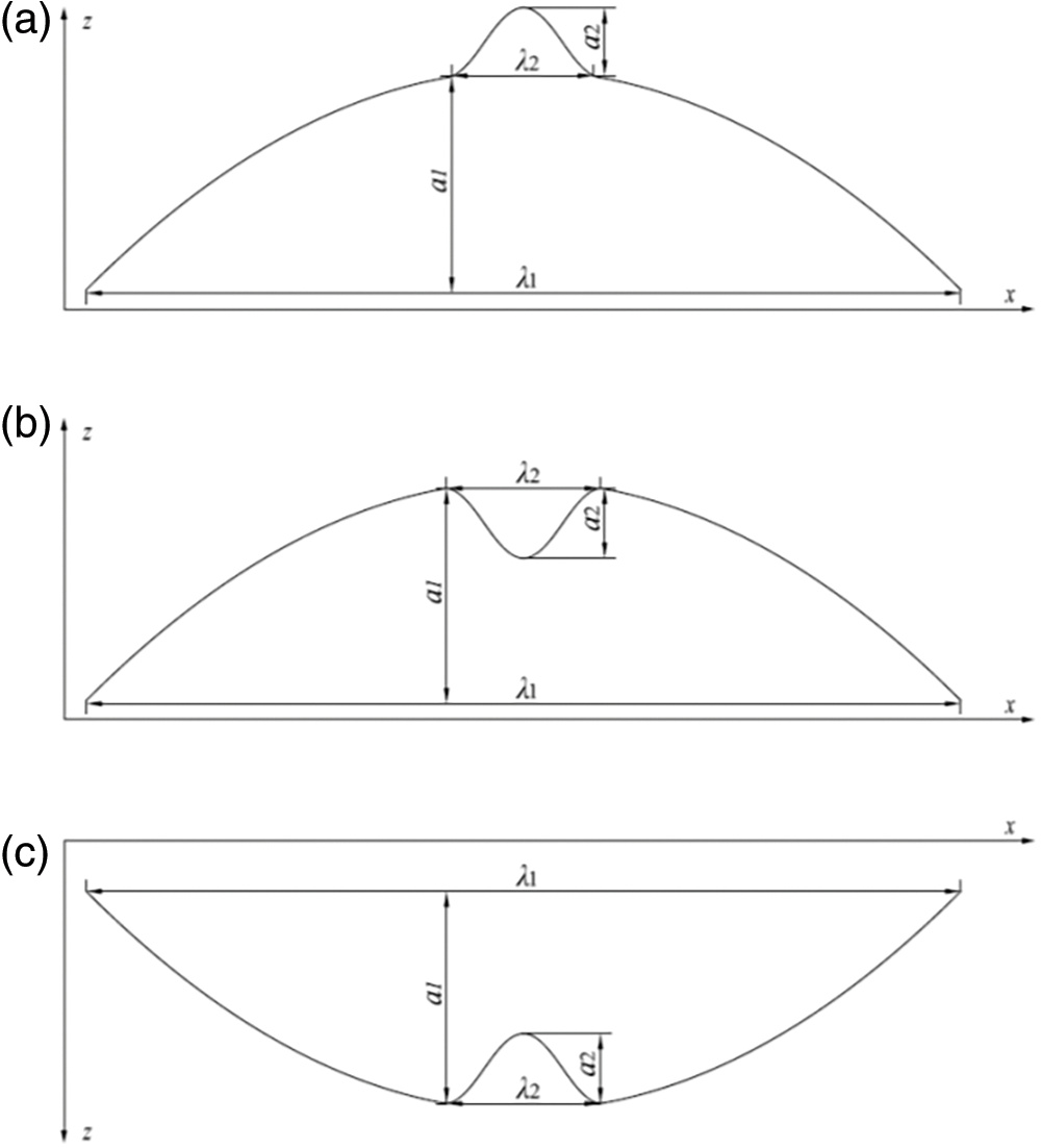
Figure 1: Wave pattern of (a) convex-A, (b) convex-B, and (c) concave rail weld irregularities

Fig. 1 clearly illustrates that the fundamental characteristic of the rail weld irregularities is a primary long-wavelength wave overlaid with a secondary short-wavelength wave. Based on field measurements, the classification of rail weld irregularity wave patterns included all types observed on the high-speed railway from Beijing to Shanghai. This classification was utilized in the present study.

2.2 Theoretical Models

In this study, three different models for rail weld irregularities are presented: the single cosine wave model [4], Gao’s model [1], and that developed in this study by modifying Gao’s model.

(1) Single-cosine wave model

For simplicity, a single cosine wave model is typically used to model the rail weld irregularity, which is expressed by Eq. (1):

z0(t)=a2[1−cos⁡(2πvt/λ)],(1)

where z0(t) represents the vertical displacement induced by irregularities at rail welds, a and λ are the amplitude and half-wavelength of the irregularities, respectively, t is time, and v is the train speed.

(2) Gao’s model

Gao et al. proposed a more precise model to simulate the geometric features of rail weld irregularities, utilizing extensive rail surface measurements on the high-speed railway from Beijing to Shanghai. It comprises three wave patterns, that is, convex-A, convex-B, and concave (see Fig. 1), and is expressed in Eqs. (2)–(4), respectively [1].

z0(t)={12a1(1−cos⁡2πvtλ1)(0≤t≤λ1−λ22v)a1+12a2[1−cos⁡2πvλ2(t−λ1−λ22v)](λ1−λ22v<t≤λ1+λ22v)12a1(1−cos⁡2πvtλ1)(λ1+λ22v<t≤λ1v),(2)

z0(t)={−12a1(1−cos⁡2πvtλ1)(0≤t≤λ1−λ22v)−a1+12a2[1−cos⁡2πvλ2(t−λ1−λ22v)](λ1−λ22v<t≤λ1+λ22v)−12a1(1−cos⁡2πvtλ1)(λ1+λ22v<t≤λ1v),(3)

z0(t)={12a1(1−cos⁡2πvtλ1)(0≤t≤λ1−λ22v)a1−12a2[1−cos⁡2πvλ2(t−λ1−λ22v)](λ1−λ22v<t≤λ1+λ22v)12a1(1−cos⁡2πvtλ1)(λ1+λ22v<t≤λ1v),(4)

where z0(t), v, and t have similar physical meanings as those in Eq. (1). a1 and a2 are the amplitudes of the primary and secondary waves, respectively. λ1 and λ2 are the half-wavelengths of the primary and secondary waves, respectively. It is worth noting that the half-wavelength of the main wave was 1 m in this study because the measurements were performed on a 1-m-long base.

(3) Proposed modified Gao’s model

In this study, a novel model was developed using a parabolic function instead of the cosine function used in Gao’s model to simulate the primary wave of rail weld irregularities. The three wave patterns of rail weld irregularities are expressed by Eqs. (5)–(7), respectively.

z0(t)={4a1t(λ1v)(1−t(λ1v))(0≤t≤λ1−λ22v)a1+12a2[1−cos⁡2πvλ2(t−λ1−λ22v)](λ1−λ22v<t≤λ1+λ22v)4a1t(λ1v)(1−t(λ1v))(λ1+λ22v<t≤λ1v),(5)

z0(t)={−4a1t(λ1v)(1−t(λ1v))(0≤t≤λ1−λ22v)−a1+12a2[1−cos⁡2πvλ2(t−λ1−λ22v)](λ1−λ22v<t≤λ1+λ22v)−4a1t(λ1v)(1−t(λ1v))(λ1+λ22v<t≤λ1v),(6)

z0(t)={4a1t(λ1v)(1−t(λ1v))(0≤t≤λ1−λ22v)a1−12a2[1−cos⁡2πvλ2(t−λ1−λ22v)](λ1−λ22v<t≤λ1+λ22v)4a1t(λ1v)(1−t(λ1v))(λ1+λ22v<t≤λ1v),(7)

where all the symbols from Eqs. (5)–(7) have similar physical meanings as those from Eqs. (2)–(4).

2.3 Comparison of Model Geometry Characteristics

A comparison of the geometric characteristics that were measured and simulated using convex-A, convex-B, and concave irregularities is illustrated in Fig. 2. It should be noted that the measured geometry characteristics of the irregularities can be referred to in the Literature [1].

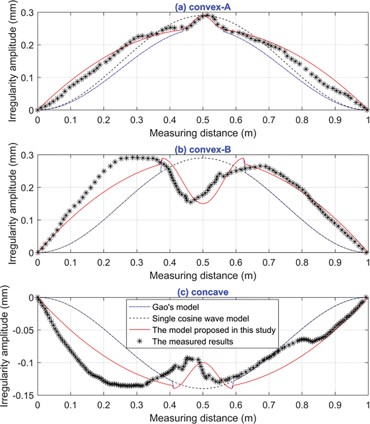
Figure 2: Comparison of geometric characteristics that were measured and modeled based on (a) convex-A, (b) convex-B, and (c) concave irregularities

As observed in Fig. 2, the single cosine wave model mainly concerns the maximum value of the irregularities at rail welds on the one hand, which could not describe the geometric shapes accurately, especially that of the secondary wave. On the other hand, Gao’s model, and that proposed in this study focused on the maximum value and the geometric shapes of the irregularities, which described the main and secondary waves precisely. As illustrated in Fig. 2, among the three theoretical models, the proposed model best matches the geometric characteristics of the measured irregularities.

The fitting accuracy of the three models is described by root mean square error (RMSE) that is expressed in Eq. (8).

RMSE=1n∑i=1n(yi−y^i)2,(8)

where yi is the amplitude of the measured irregularity, y^i is the simulated amplitude of the irregularity and n is the number of measurement data along the measuring distance.

The RMSE of the simulated amplitudes of the irregularity corresponding to the measured irregularity amplitude are listed in Table 1. It is clearly shown that the proposed model has the smallest RMSE value, which means the proposed model has better fitting accuracy than the other two simulating models.

3  Wheel-Rail Vertical Dynamic Force Induced by Irregularities at Rail Welds

To show the effectiveness of the proposed rail weld irregularity model, the three theoretical models and measured data for the rail weld irregularities (see Fig. 2) illustrated in the previous section were implanted into the vehicle-track coupled dynamic model to simulate the wheel/rail vertical dynamic responses. Further, the calculated results at different train speeds of 300, 350, and 400 km/h were analyzed and compared in the time and frequency domains.

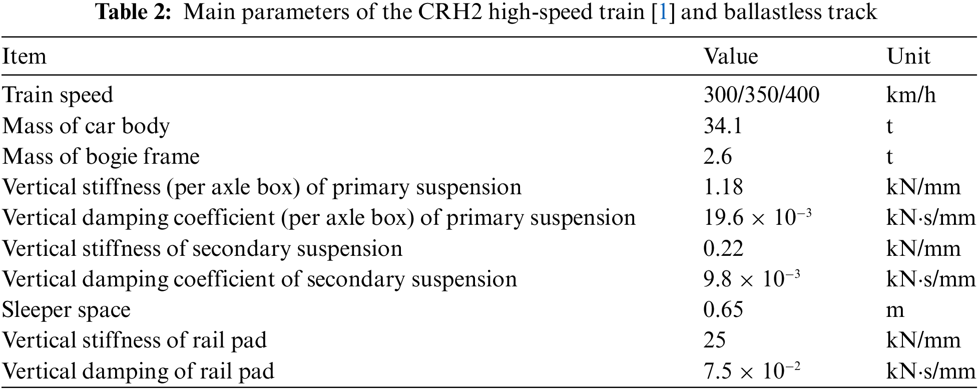
The dynamic model was developed in NUCARS® which is commercial multi-body dynamics software consisting of 7 rigid bodies and 42 degrees of freedom. The car body, wheelsets, and bogie frame are simulated as rigid bodies, and the rail is simplified as a Timoshenko beam. The parameters of the CRH2 high-speed train in China [1] and the ballastless track adopted in this study are listed in Table 2.

According to the measured geometric characteristics of various types of rail weld irregularities, the parameters for the three modeled irregularities were determined. a1 is 0.25, 0.29, and 0.14 mm, a2 is 0.04, 0.14, and 0.04 mm, λ1 is 1.0, 1.0, and 1.0 m, and λ2 is 0.12, 0.25, and 0.18 mm for convex-A, convex-B, and concave irregularities, respectively, which can be referred to those in the literature [1].

3.1 Comparison of Time Domain Response

The results of wheel-rail vertical dynamic force induced by the three types of rail weld irregularities both modeled and measured, are shown in Figs. 3–5, respectively. They have been compared and discussed to verify the effectiveness of the proposed model.

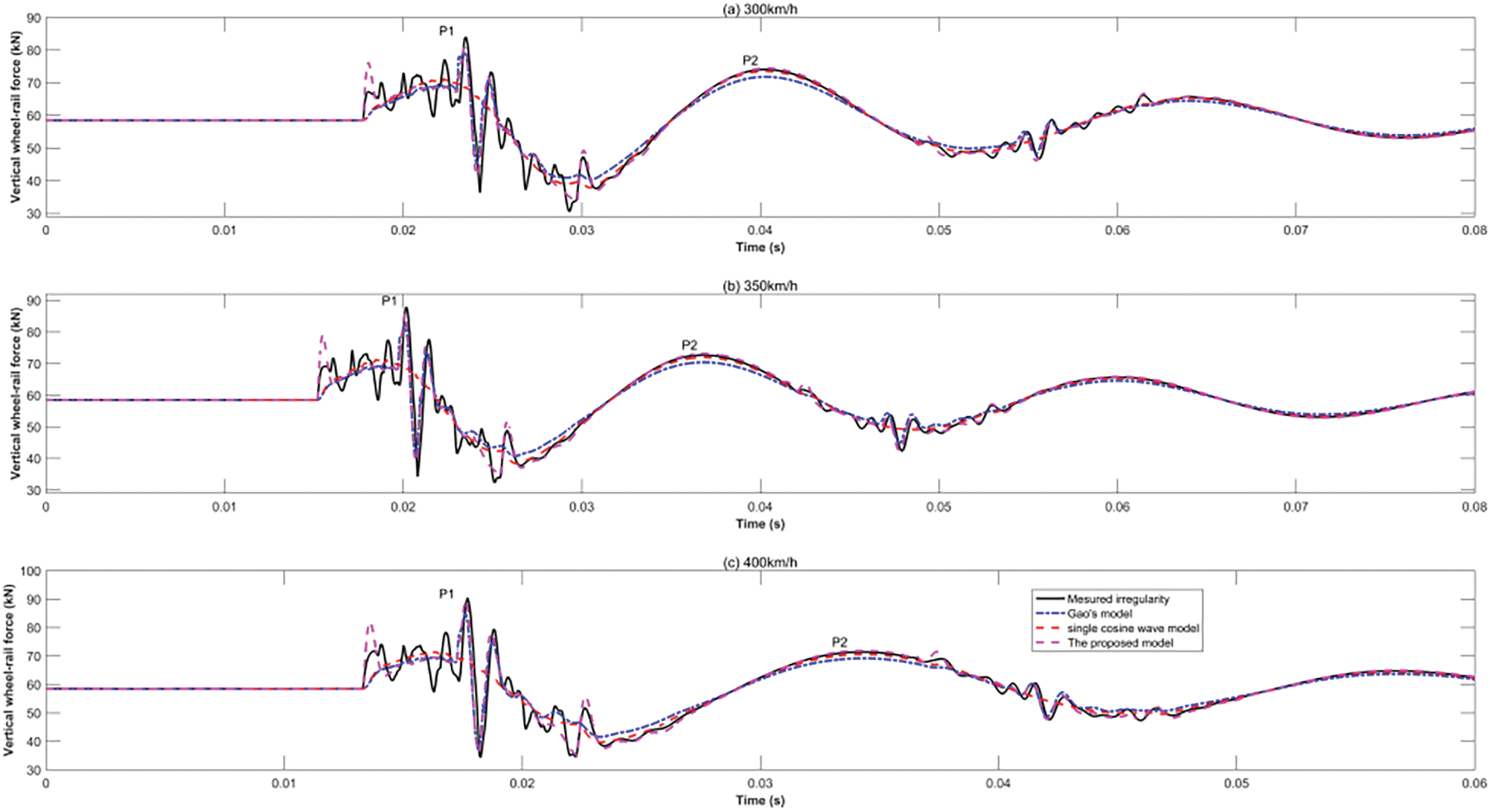
Figure 3: Comparison of vertical force induced by convex-A irregularities at train speeds of (a) 300, (b) 350, and (c) 400 km/h

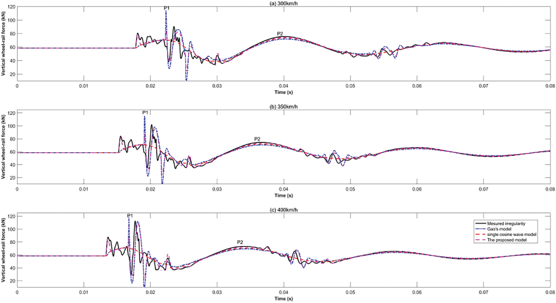
Figure 4: Comparison of vertical force induced by convex-B irregularities at train speeds of (a) 300, (b) 350, and (c) 400 km/h

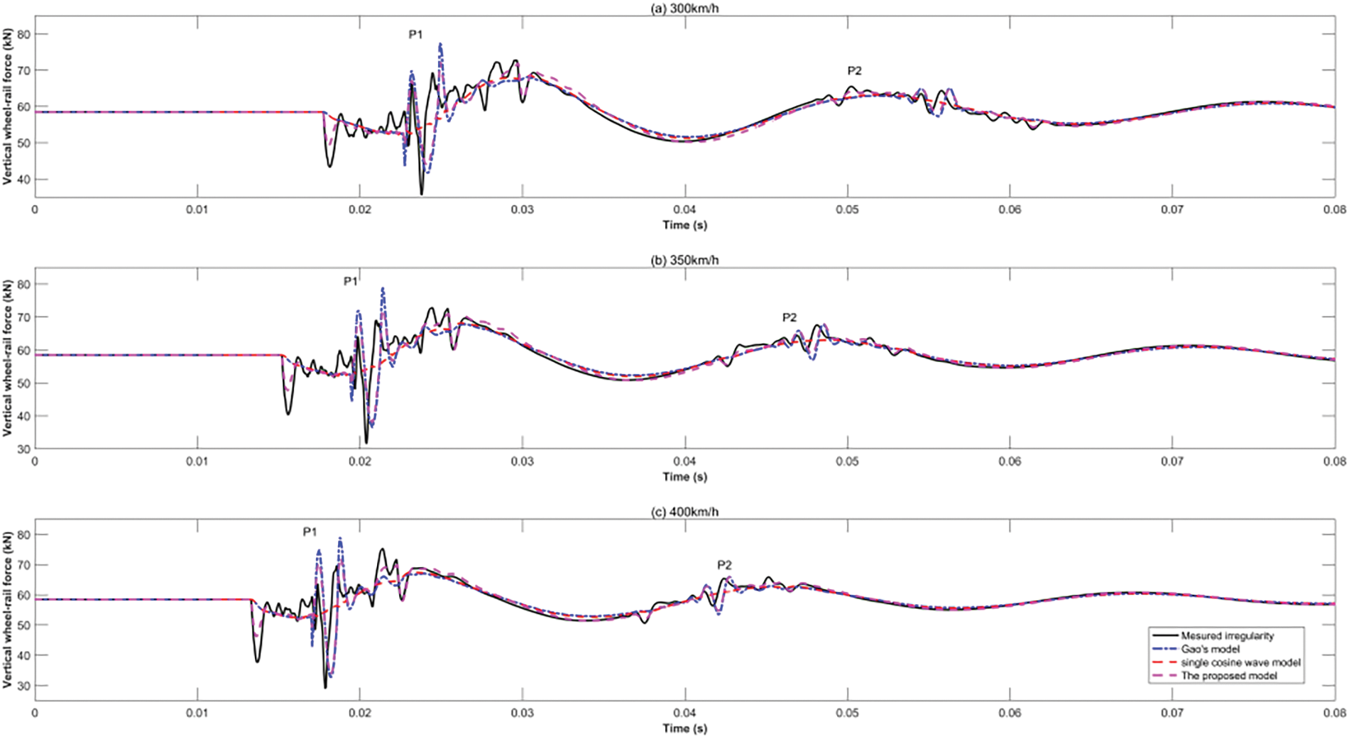
Figure 5: Comparison of vertical force induced by concave irregularities at train speeds of (a) 300, (b) 350, and (c) 400 km/h

As illustrated in Figs. 3–5, the low-frequency P2 impact force in the time domain was simulated excellently for both the vibration waveform and maximum value using all three theoretical models. For the high-frequency P1 impact force in the time domain, the single cosine wave model captured neither the maximum values nor the vibration waveforms for all three types of rail weld irregularities, which may have been due to a disregard of the secondary wave for the measured irregularities. Gao’s model obtained good results for convex-A irregularities but was not good for convex-B and concave irregularities, which may be owing to the large gap in the amplitude value between the primary and secondary waves (see Fig. 2). The proposed model achieved good results for all three patterns of rail weld irregularities, whether in terms of waveform or maximum value.

The error band between the amplitudes of the impact forces P1 and P2 induced by irregularities that were measured and modeled was analyzed, as illustrated in Fig. 6. It is worth noting that the legends for convex-A, convex-B, and concave irregularities are represented by the black, blue and red symbols, respectively.

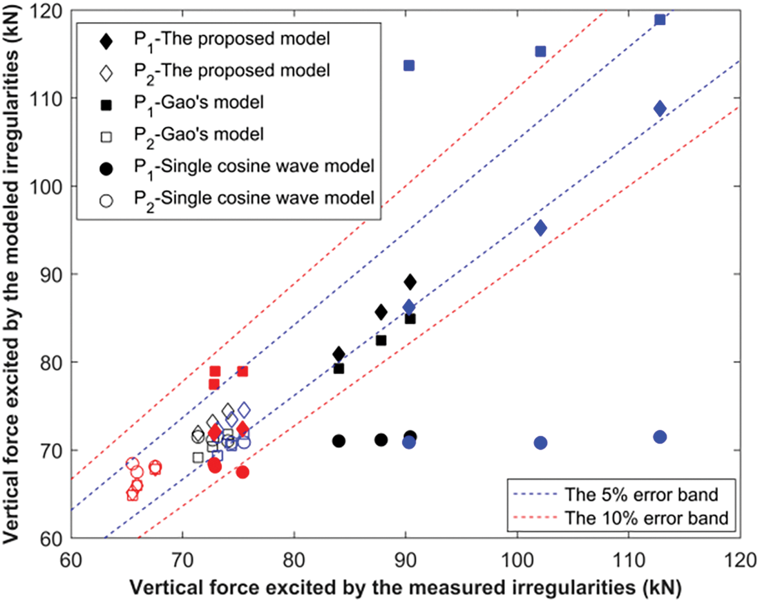
Figure 6: The error band between the results that were induced by the measured and modeled irregularities

Fig. 6 shows that the low-frequency P2 impact forces in the time domain simulated by all three theoretical models were almost all located within the 5% error band. For the high-frequency P1 impact force in the time domain, the simulated results of the proposed model for the three types of rail weld irregularities were almost all located within the 5% error band. The results simulated by Gao’s model were almost all located within the 10% error band, except for the convex-B irregularities. The results simulated by the single cosine wave model were all located outside the 10% error band.

Hence, from Figs. 3–6, it can be concluded that the proposed model was more appropriate for describing the vertical dynamic force than the single cosine wave model and Gao’s model, whether in the vibration waveform or amplitudes of the impact forces P1 and P2 in the time domain.

3.2 Comparison of Frequency Domain Response

To further verify the effectiveness of the proposed model used in describing rail weld irregularities, the vertical dynamic forces caused by the measured and modeled irregularities in the frequency domain were analyzed and compared. The vertical dynamic forces in the frequency domain were obtained and compared using the fast Fourier transform (FFT) of the forces in the time domain shown in Figs. 3–5, which are illustrated in Figs. 7–9.

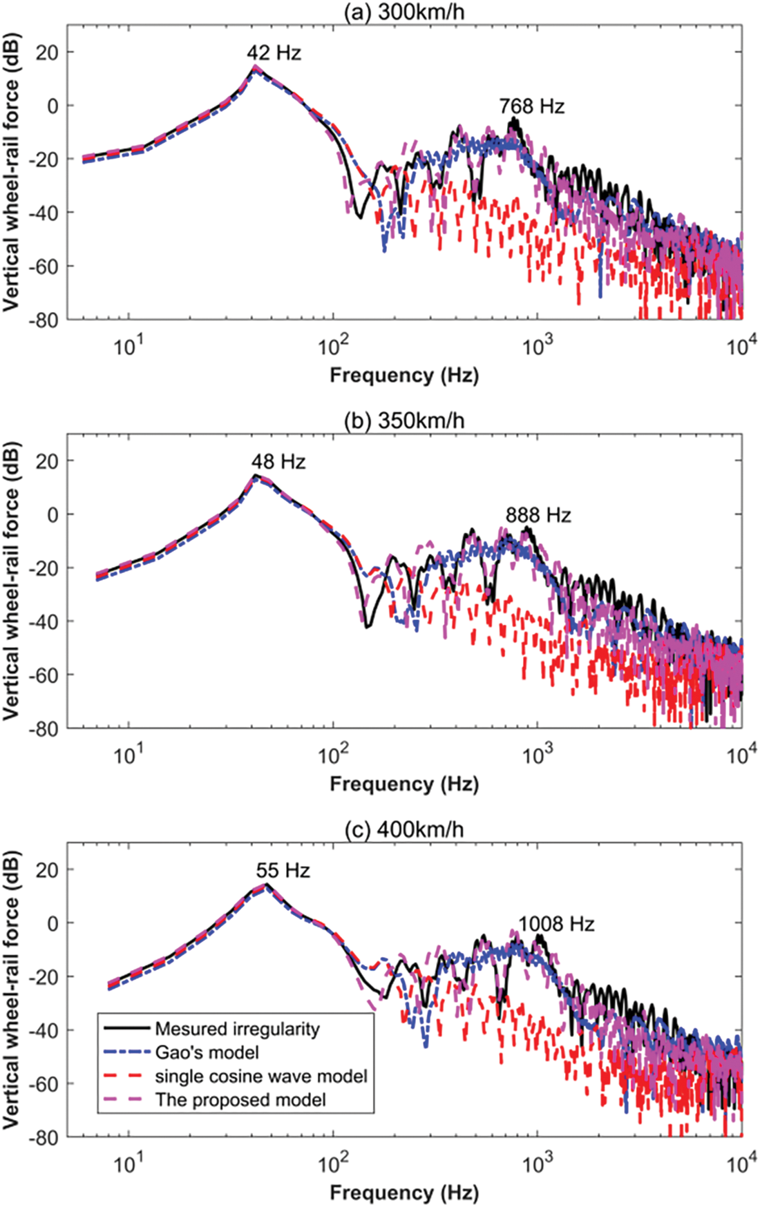
Figure 7: Comparison of vertical forces in the frequency domain induced by convex-A irregularities at train speeds of (a) 300, (b) 350, and (c) 400 km/h

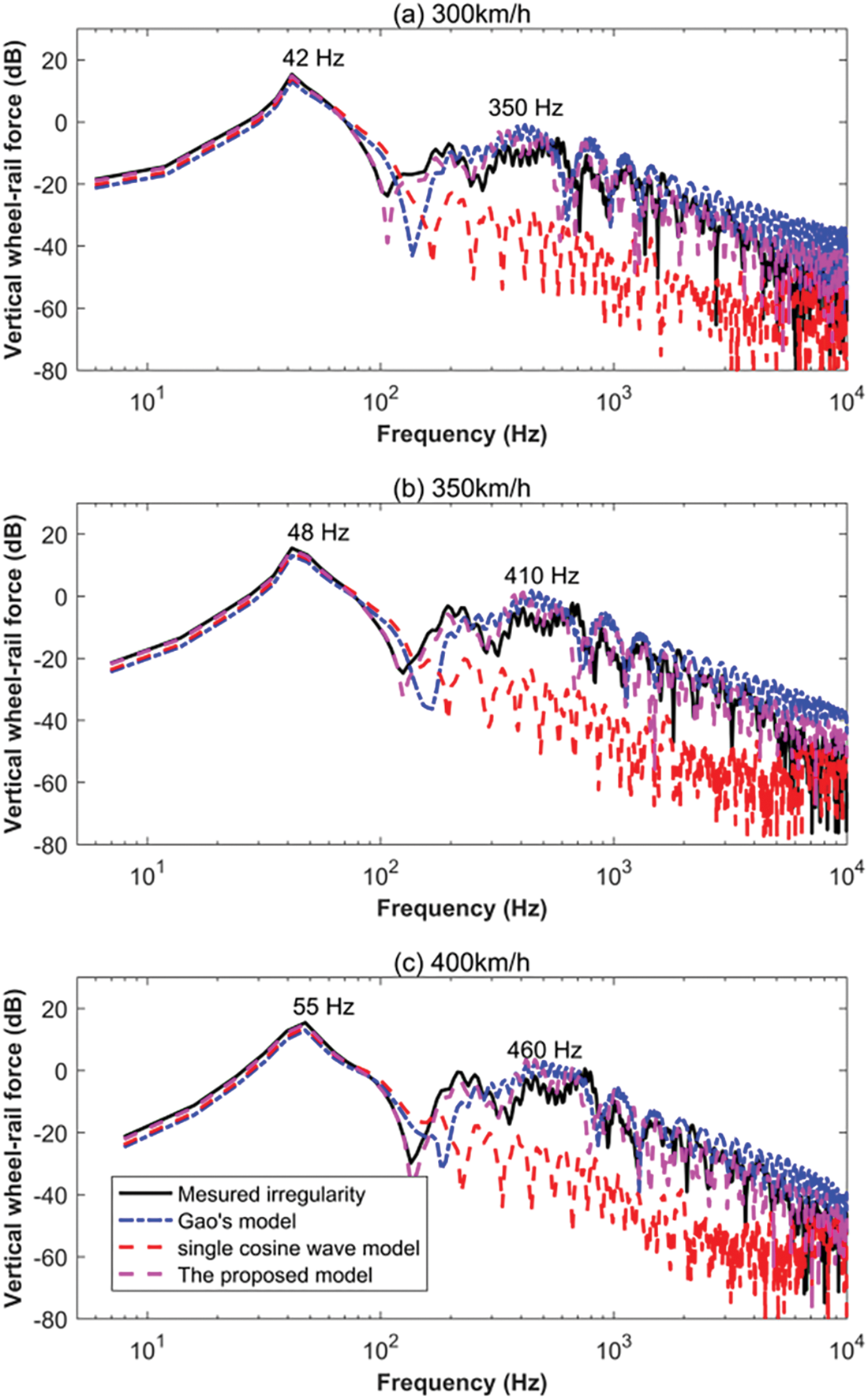
Figure 8: Comparison of vertical force in the frequency domain induced by convex-B irregularities at train speeds of (a) 300, (b) 350, and (c) 400 km/h

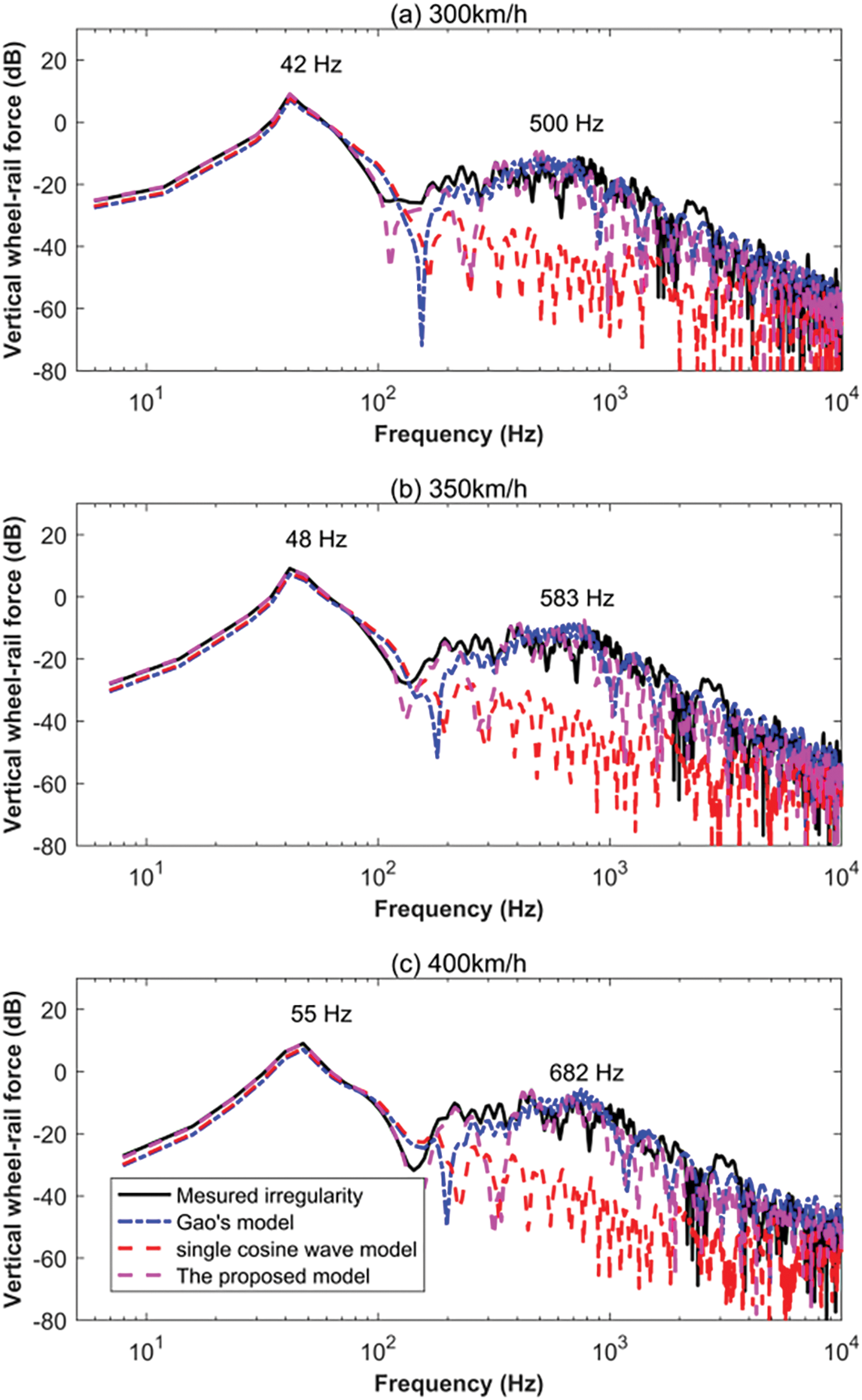
Figure 9: Comparison of vertical force in the frequency domain induced by concave irregularities at train speeds of (a) 300, (b) 350, and (c) 400 km/h

From Figs. 7–9, it was observed that the frequency of the vertical dynamic force was divided into two distinct bands by the frequency value of 100 Hz, which corresponds to the results obtained in the Literature [1]. One was in the low-frequency region, which reflected the impact force P2 caused by the primary long-wavelength irregularity. The other was situated in the high-frequency region, representing the impact force P1 excited by the secondary short-wavelength irregularity.

For the low-frequency impact force P2, the vibration frequencies induced by the measured irregularities were like those of the irregularities modeled by all three theoretical models. This showed good simulation results for the low-frequency impact force P2 in the frequency domain by all three theoretical models. The vibration frequencies associated with the low-frequency impact force P2 were consistent across all three types of irregularities, indicating a shared characteristic among them in exciting similar vibration frequencies. The frequency range of P2 force is concentrated between 42 to 55 Hz.

For the high-frequency impact force P1, the vibration frequencies varied from 400 to 1000 Hz for the three types of rail weld irregularities. The vertical forces in the frequency domain caused by the proposed rail weld irregularity models corresponded closely to those induced by the measured irregularity, outperforming those induced by Gao’s model and the single cosine wave model. The vibration frequencies for the high-frequency impact force P1 under different train running speeds of 300, 350, and 400 km/h satisfied Eq. (9), which means that the vibration frequency was proportional to the speed and inversely proportional to the irregularity wavelength. Hence, the vibration frequencies of the impact force P1 induced by the convex-A rail weld irregularities were the highest, followed by those caused by concave irregularities. The results caused by the convex-B rail weld irregularities were the lowest, owing to the longest wavelength of the secondary wave for the convex-B rail weld irregularities adopted in this study.

f=vλ.(9)

4  Machine Learning Models Based on Coupled Vehicle-Track Dynamics Models

In this section, an Artificial Neural Network (ANN) machine learning model is presented, which is combined with a coupled vehicle-rail dynamics model for predicting the impact force P1 and P2 due to rail weld irregularities. The dataset used for the training of the ML model is created by numerical simulation. Subsequently, prediction of the impact forces due to rail weld irrregularities and parameter tuning were performed. It is impractical to rely solely on experimental or numerical simulations to obtain the impact force due to weld upset for each complex operating condition. To address this limitation, we have developed an ML model based on a coupled vehicle-rail dynamics model designed to quickly and adaptively acquire the properties of the structure. The model combines the advantages of the coupled vehicle-rail dynamics approach and the ML model to acquire the properties of the structure in a more efficient way to predict the vertical forces on the wheel-rail due to rail weld irrregularity.

4.1 Artificial Neural Network models

ANN is a computational model that mimics the structure and function of biological neural networks for processing and analyzing complex data. It mimics the workings of the human brain through a large number of simple nodes (called neurons or units) and their interconnections. ANN has powerful learning capabilities and has several advantages over other machine learning models (Support Vector Machines (SVM) and Random Forests (RF), etc.): (1) Handling complex nonlinear relationships. ANN can capture complex nonlinear relationships in data through multiple hidden layers and nonlinear transfer functions (e.g., ReLU, Sigmoid, Tanh, etc.). Compared to linear models, ANN can fit complex data more accurately. (2) Adaptive learning capability. ANN can minimize the loss function by continuously adjusting the model parameters (weights and biases). This process is adaptive and can automatically optimize the model according to the characteristics of the data and gradually improve the prediction performance. (3) Efficient parallel computing. The computational process of ANN involves a large number of matrix operations, which can be efficiently parallelized and executed on modern computing devices (e.g., GPU, TPU). This makes ANN have high computational efficiency when dealing with large-scale data.

ANN performs well in many applications, but they also have some limitations and challenges: ANN are often regarded as “black-box” models, and their internal structure and decision-making process are difficult to explain; ANN usually require a large amount of data for training, and may not perform well for tasks with a small amount of data; the training of ANN involves the tuning of many hyperparameters (e.g., learning rate, number of neurons, number of network layers, etc.), and finding the optimal combination of hyperparameters usually requires a lot of experimentation and debugging.

As shown in Fig. 10 below, the basic structure of ANN consists of three parts. (1) Input layer: receives raw data input. (2) Hidden layer: located between the input layer and the output layer and consists of a set of neurons. A neural network can have one or more hidden layers, and the number of layers and the number of neurons in each layer depends on the specific application. (3) Output layer: generates the final model output.

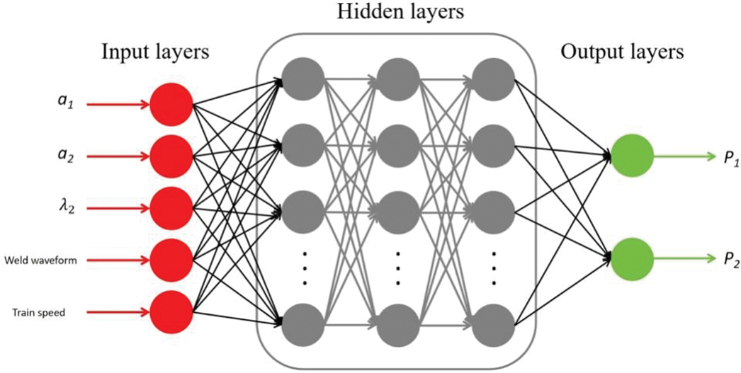
Figure 10: The basic structure of ANN

The input data is passed through the input layer to the hidden layer and then through the hidden layer to the output layer. After processing the input information vector X, the neuron uses the transfer function f to produce the output Y:

Y=f(w⋅X+b),(10)

where w and b represent the weights and biases of the neurons, respectively. The transfer function f can have various forms, including linear function, sigmoid function, and ReLU function. The training of the AI network relies on the Adam optimization algorithm. Adam is an adaptive learning rate optimization algorithm that combines the advantages of the Momentum and Root Mean Square Propagation (RMSprop) algorithms, aiming to efficiently deal with sparse and noisy gradients to speed up model convergence and improve performance.

The main steps of Adam’s optimization algorithm are to initialize the values of the parameters first-order moment estimation (momentum variable) and second-order moment estimation (squared gradient variable), followed by iterations to update the parameters, and in each iteration to compute the current gradient, gt:

gt=∇θft(θt−1),(11)

where ∇θ represents the gradient of the parameter θ and ft(θt−1) is the objective function being optimized. Followed by first-order moment estimation, mt, and second-order moment estimation, vt:

mt=β1⋅mt−1+(1−β1)⋅gt,(12)

vt=β2⋅vt−1+(1−β2)⋅gt2,(13)

The default values of the momentum parameters β1 and β2 are 0.9 and 0.999, respectively.

Since the values of mt and vt are biased towards 0 in the initial phase, a bias correction is also required:

m^t=mt1−β1t,(14)

v^t=vt1−β2t,(15)

Finally, the update of the parameter θt is performed:

θt=θt−1−αv^t+∋⋅m^t,(16)

where the learning rate α has a default value of 0.001 and ∋ is a very small number, usually 10−8, used to prevent division by zero errors. The training process is completed when the change in the objective function (e.g., loss function) defined in the machine learning model is less than a certain threshold after many iterations by stopping the iterations.

4.2 Establishment of the Database

This study involves the construction, training, and validation of an ANN model using the Python programming language. The model will include the important variables related to the generation of impact forces, i.e., the parameters associated with the weld upset modeled in this paper (a1, a2, and λ2), the different types of welds (convex-A, convex-B, and concave), and the speed at which the train is running. The outputs include impact forces P1 and P2. Firstly, the individual features in the database were analyzed for correlation, the correlation coefficient is defined as the covariance of two features divided by the product of their standard deviations:

r(X,Y)=Cov(X,Y)Var[X]Var[Y],(17)

where Cov(X,Y) is the covariance between two features X and Y, Var[X] is the variance of X, and is the variance of Y. If the correlation coefficient is greater than 0.5, the two features are considered to be related to each other. As shown in Fig. 11 below, the correlation coefficients are shown in the form of a heat map. From the figure, it can be seen that the correlation coefficients between the five input features are very small and they are considered to be uncorrelated, but there is considered to be a weak positive correlation between the correlation parameter a1 of the weld unevenness model and the low-frequency impact force P2, and a positive correlation between the correlation parameter a2 of the weld unevenness model and the high-frequency impact force P1. The results show that this model can be trained using an artificial neural network model.

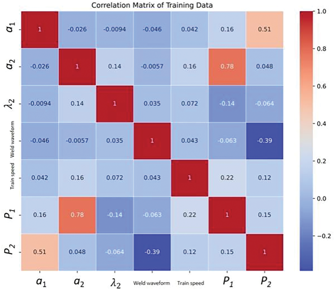
Figure 11: Heat map of correlation between different features

A total of 252 sets of data on the impact force P1 and P2 due to weld unevenness under various conditions were collected using the coupled vehicle-rail dynamics method, where the models used included both the directly measured model and the modified Gao’s model proposed in this paper. These data are randomly disrupted and divided in a ratio of 7:3, where 176 groups are used for training and the remaining 76 groups are used for testing. To reduce significant differences between the input data, the data is normalized before it enters the hidden layer. This normalization process helps to mitigate the potential impact of individual data points on network training.

4.3 Parameter Optimization and Prediction of Impact Forces

The prediction results of a model are significantly affected by the internal structure and hyperparameters of the model. For ANN models, several hyperparameters must be determined, such as the selection of an appropriate activation function, the number of hidden layers, and the number of neurons within each hidden layer. The quality of the model parameters is assessed based on metrics such as RMSE and regression coefficient (R2). These metrics are benchmarks for evaluating the accuracy and goodness of fit of the model. The smaller the RMSE value or the closer the R2 value is to 1, the higher the quality of the model. The equation for RESM is shown in Eq. (8) and R2 is calculated as follows:

R2=∑i=1n(y^i−y¯)2∑i=1n(yi−y¯)2,(18)

where yi is the expected value, y^i is the predicted value, y¯ is the mean of the expected value, and n is the number of samples.

The commonly used transfer functions in ANN include ReLU, Sigmoid, and Tanh. Among them, ReLU function is simple to compute and efficient, which can alleviate the problem of gradient vanishing and make the deep network training more efficient; the Sigmoid function can reduce the influence of extreme values and make the model more stable; Tanh has a wider dynamic range, which can allow the gradient descent algorithm to converge faster and can capture nonlinear patterns well. In this study, we adopt the ReLU function as the transfer function.

The training process of the ANN model in this paper uses an early stopping mechanism, i.e., when the loss function in the model (which is defined as the root mean spuare error RMSE in this model) no longer improves within a specified number of iterations, the training stops to avoid overfitting. In this paper, training is stopped if the loss function of the validation set does not improve within 100 iterations. As an example, the hidden layer is 3 layers, and the iterative process of the model is shown in Fig. 12.

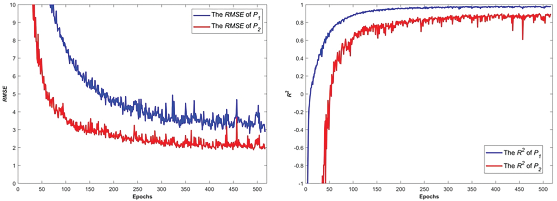
Figure 12: Variation process of RMSE and R2 with the number of iterations

The choice of the number of hidden layers and the allocation of neurons within each hidden layer need to be discussed in detail when exploring the optimal values of the ANN model parameters.

There are three commonly used numbers of hidden layers in AI network architectures: 2, 3, and 4. Increasing the number of hidden layers enhances the ability of the network to be able to learn more complex and abstract representations of features, thus helping to capture nuances and complex patterns in the data. However, this increase can lead to an increase in training time, and deeper networks are more likely to suffer from the problem of vanishing or exploding gradients, which may overfit the training data and lead to training difficulties. The effect of different numbers of hidden layers (2, 3, and 4) on the prediction accuracy of the neural network was comparatively evaluated in predicting the impact force due to rail weld irrregularity. The error band plots shown in Fig. 13 show that the neural network reaches its best performance when 3 hidden layers are used. Most of the data points are very close to the diagonal (y = x) and only a small fraction of the points deviates from the 5% relative error band.

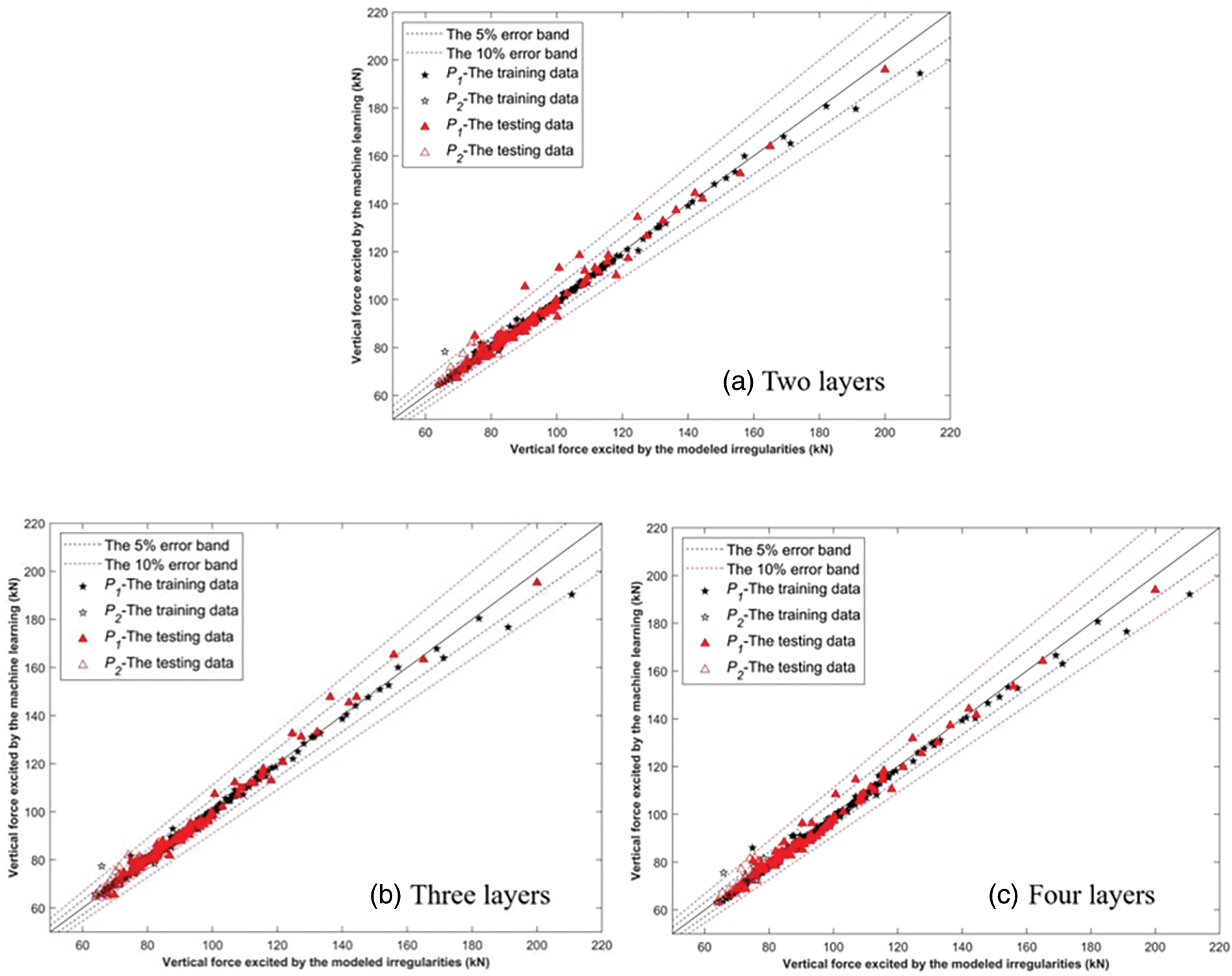
Figure 13: ANN prediction results for different number of hidden layers: (a) two layers; (b) three layers; (c) four layers

In terms of the number of neurons, the number of neurons in the first layer plays a crucial role in determining the predictive performance of the ANN. We investigated the range of 20 to 100 neurons in the first layer. As shown in Fig. 14, the best performance was obtained when the first layer consisted of 34 neurons, and the sum of the root mean square errors of the two target values was 4.49. Similarly, the number of neurons in the other two layers was investigated using the same methodology. The optimal structural parameters for predicting the impact force model due to rail weld irrregularity in this study were most obtained, as shown in Table 3.

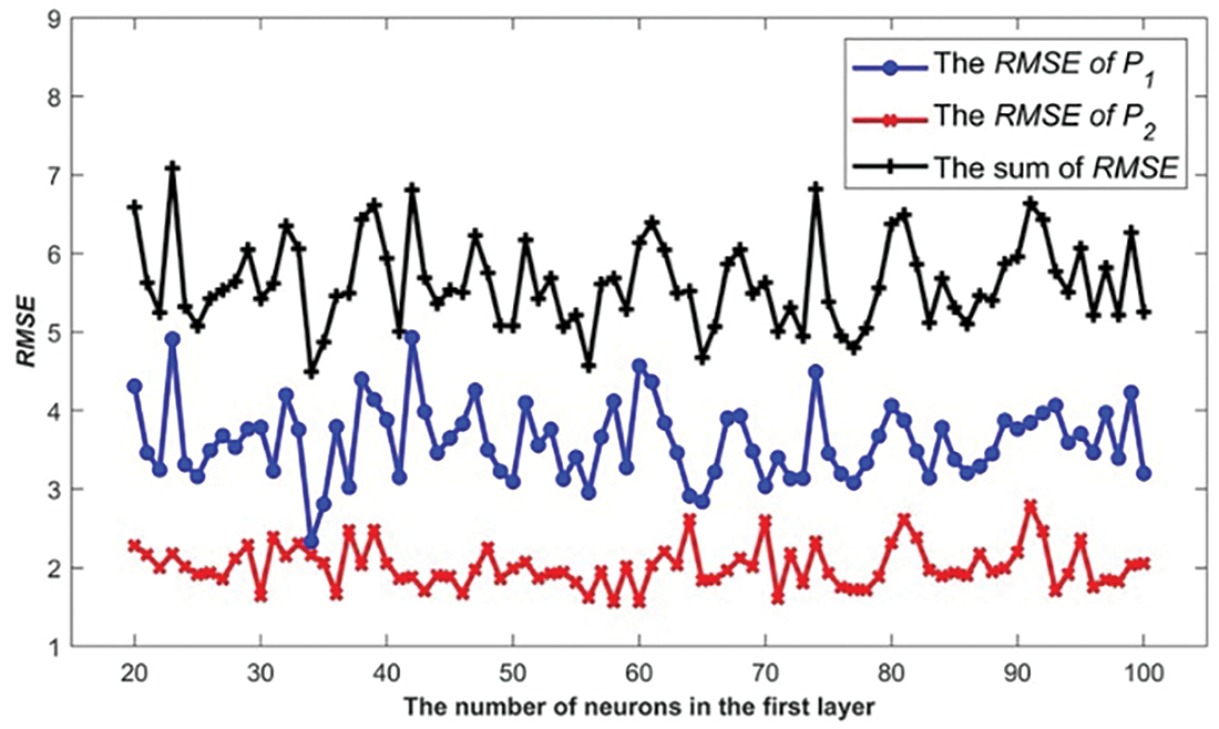
Figure 14: Variation of the value of RMSE with the number of neurons in the first hidden layer

After obtaining the optimal structural parameters of the ANN model, we analyzed the testing data from the test set, which had been randomly divided earlier, and which consisted of the prediction of the impact force due to the rail weld irrregularity using two models (the measured weld irregularities model and the use of the high-style modification model proposed in this paper). The error band diagrams of the data from the test set are shown in Fig. 15. From the figure, we can see that the data predicted by the optimized machine learning model in the testing set are all within the 10% error band, and the impact forces predicted by the model for the measured weld irregularities are all within the 5% error band, and it can be seen that the optimized machine learning model based on the coupled vehicle-rail dynamics model is good for predicting the impact forces due to the rail weld irrregularity.

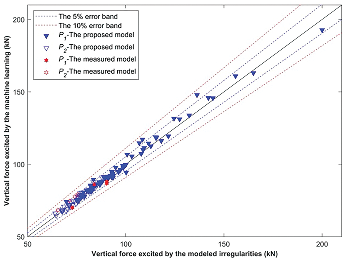
Figure 15: Error band diagram of optimised testing set data

5  Conclusions

In this study, a novel theoretical model was developed for describing the geometric wave patterns of rail weld irregularities that occurred in the high-speed railways of China. The vertical dynamic forces under different running speeds, which were induced by the rail weld irregularities that were measured and modeled, were calculated using the vehicle-track coupled dynamic model. The effectiveness of the proposed model was verified by comparing the vertical dynamic force in the time and frequency domains, which were induced by rail weld irregularities that were measured and modeled using three different theoretical models. The following conclusions can be drawn:

(1)   To obtain precise results for the impact wheel/rail forces P1 and P2, the maximum value and geometric shapes of the rail weld irregularities were considered in the theoretical model.

(2)   The vibration waveform and amplitudes of the impact forces P1 and P2, which were excited by rail weld irregularities, were described more precisely using the proposed model in this study, both in the time and frequency domains, than those described using the single cosine wave model or Gao’s model.

(3)   The vibration frequency variation ranging from 400 to 1000 Hz and 40 to 60 Hz for the high- and low-frequency impact forces P1 and P2, respectively, were excited using the three types of rail weld irregularities under train running speeds of 300 to 400 km/h.

(4)   The vibration frequency of the high-frequency impact force P1 is proportional to the train running speed and inversely proportional to the irregularity wavelength of the secondary wave.

(5)   The ANN model based on vehicle-rail coupling dynamics is established, and the correlation coefficients are analyzed to obtain a weak positive correlation between the correlation parameter a1 of the weld unevenness model and the low-frequency impact force P2, and a positive correlation between the correlation parameter a2 of the weld unevenness model and the high-frequency impact force P1. The optimal parameters are finally determined through detailed analyses to achieve the effective prediction of the impact force due to the track weld unevenness while reducing the computation time.

(6)   Limitations of this article. The classification of rail weld irregularities in the study is based on empirical data from the Beijing-Shanghai High-Speed Railway, which may not fully represent the types of rail weld irregularities found in other high-speed railway lines in China or high-speed railway lines worldwide. Furthermore, due to the “black box” nature of the ANN model, the interpretability of the model is poor, so a method of interpreting the model should be explored to achieve efficient prediction while effectively interpreting the relationship between input and output variables.

Acknowledgement: The authors wish to express their appreciation to the reviewers for their helpful suggestions which greatly improved the presentation of this paper.

Funding Statement: This study was supported by Natural Science Foundation of China (52178441) and the Scientific Research Projects of the China Academy of Railway Sciences Co., Ltd. (Grant No. 2022YJ043).

Author Contributions: The authors confirm contribution to the paper as follows: conceptualization, Linlin Sun and Zihui Wang; methodology, Linlin Sun; software, Shukun Cui; validation, Shukun Cui and Ziquan Yan; formal analysis, Linlin Sun and Zihui Wang; investigation, Weiping Hu and Qingchun Meng; resources, Shukun Cui; data curation, Zihui Wang; writing—original draft preparation, Linlin Sun and Zihui Wang; writing—review and editing, Ziquan Yan; visualization, Weiping Hu; supervision, Ziquan Yan. All authors reviewed the results and approved the final version of the manuscript.

Availability of Data and Materials: The data that support the findings of this study are available from the corresponding author upon reasonable request.

Ethics Approval: Not applicable.

Conflicts of Interest: The authors declare no conflicts of interest to report regarding the present study.

References

1. Gao JM, Zhai WM, Guo Y. Wheel-rail dynamic interaction due to rail weld irregularity in high-speed railways. Proc Inst Mech Eng Part F: J Rail Rapid Transit. 2018;232(1):249–61. doi:10.1177/0954409716664933. [Google Scholar] [CrossRef]

2. Kouroussis G, Connolly DP, Verlinden O. Railway-induced ground vibrations—A review of vehicle effects. Int J Rail Transport. 2014;2(2):69–110. doi:10.1080/23248378.2014.897791. [Google Scholar] [CrossRef]

3. An BY, Wang P, Xiao JL, Xu JM, Chen R. Dynamic response of wheel-rail interaction at rail weld in high-speed railway. Shock Vib. 2017;2017(1):5634726. doi:10.1155/2017/5634726. [Google Scholar] [CrossRef]

4. Niu LB, Zhao J, Liu JZ. Wheel-rail vertical force characteristics under rail welded joint excitation. Railway Eng. 2020;60(9):5 (In Chinese). [Google Scholar]

5. Esveld C. Modern railway track. 2nd ed. Zaltbommel, The Netherlands: Delft University of Technology; 2001. [Google Scholar]

6. Mutton PJ, Alvarez EF. Failure modes in aluminothermic rail welds under high axle load conditions. Eng Fail Anal. 2004;11(2):151–66. doi:10.1016/j.engfailanal.2003.05.003. [Google Scholar] [CrossRef]

7. Zhai W, Wang Q, Lu Z, Wu X. Dynamic effects of vehicles on tracks in the case of raising train speeds. Proc Inst Mech Eng Part F: J Rail Rapid Transit. 2001;215(2):125–35. doi:10.1243/0954409011531459. [Google Scholar] [CrossRef]

8. Sun L, Yan Z, Xiao J, Fang H, Cui S. Experimental analysis of the modal characteristics of rail fastening clips. Proc Inst Mech Eng Part F: J Rail Rapid Transit. 2020;234(2):134–41. doi:10.1177/0954409719834784. [Google Scholar] [CrossRef]

9. Lyon D. The calculation of track forces due to dipped rail joints, wheel flats and rail welds. In: Second ORE Colloquium on Technical Computer Programs, London: RSSB Ltd. 1972. [Google Scholar]

10. Jenkins HH, Stephenson JE, Clayton GA, Morland GW, Lyon D. The effect of track and vehicle parameters on wheel/rail vertical dynamic forces. Railw Eng J. 1974;3(1):2–16. [Google Scholar]

11. Steenbergen MJMM. Quantification of dynamic wheel-rail contact forces at short rail irregularities and application to measured rail welds. J Sound Vib. 2008;312:606–29. [Google Scholar]

12. Steenbergen MJMM, Esveld C. Relation between the geometry of rail welds and the dynamic wheel-rail response: numerical simulations for measured welds. Proc Inst Mech Eng Part F: J Rail Rapid Transit. 2006;220:409–23. [Google Scholar]

13. Steenbergen MJMM, Esveld C. Rail weld geometry and assessment concepts. Proc Inst Mech Eng Part F: J Rail Rapid Transit. 2006;220(3):257–71. doi:10.1243/09544097JRRT38. [Google Scholar] [CrossRef]

14. Gao JM, Zhai WM. Dynamic effect and safety limits of rail weld irregularity on high-speed railway. Scient Sin Technol. 2014;44(7):697–706 (In Chinese). doi:10.1360/N092014-00081. [Google Scholar] [CrossRef]

15. Xiao J, Yan Z, Shi J, Ma D. Effects of wheel-rail impact on the fatigue performance of fastening clips in rail joint area of high-speed railway. KSCE J Civ Eng. 2022;26(1):120–30. doi:10.1007/s12205-021-1905-9. [Google Scholar] [CrossRef]

16. Wang K, Liu P, Zhai W, Huang C, Chen Z, Gao J. Wheel-rail dynamic interaction due to excitation of rail corrugation in high-speed railway. Sci China Tech Sci. 2015;58(2):226–35. doi:10.1007/s11431-014-5633-y. [Google Scholar] [CrossRef]

17. Shi H, Zeng J, Guo J. Disturbance observer-based sliding mode control of active vertical suspension for high-speed rail vehicles. Vehicle Syst Dyn. 2024:1–24. doi:10.1080/00423114.2024.2305296. [Google Scholar] [CrossRef]

18. Zhan Z, He X, Tang D, Dang L, Li A, Xia Q, et al. Recent developments and future trends in fatigue life assessment of additively manufactured metals with particular emphasis on machine learning modeling. Fatigue Fract Eng M. 2023;46(12):4425–64. doi:10.1111/ffe.14152. [Google Scholar] [CrossRef]

19. Zhu T, Wang X, Wu J, Zhang J, Xiao S, Lu L, et al. Comprehensive identification of wheel-rail forces for rail vehicles based on the time domain and machine learning methods. Mech Syst Signal Pr. 2025;222:111635. doi:10.1016/j.ymssp.2024.111635. [Google Scholar] [CrossRef]

20. Luo J, Teng F, Zhou Y, Chi M, Zhang H. A wheel-rail force inversion model for high-speed railway. J Nanning Univ (Nat Sci). 2021;57:299–308 (In Chinese). [Google Scholar]

21. Gadhave R, Vyas NS. Rail-wheel contact forces and track irregularity estimation from on-board accelerometer data. Vehicle Syst Dyn. 2022;60(6):2145–66. doi:10.1080/00423114.2021.1899253. [Google Scholar] [CrossRef]

22. Guo J. Theory and application research on wheel rail force load identifcation based on data modeling (Ph.D. Thesis). China Academy of Railway Sciences: China; 2015 (In Chinese). [Google Scholar]

23. Graupe D. Principles of artificial neural networks. Singapore: World Scientific; 2013. [Google Scholar]

24. Athey S, Tibshirani J, Wager S. Generalized random forests. Ann Stat. 2019;47(2):1148–78. doi:10.1214/18-AOS1709. [Google Scholar] [CrossRef]

25. Kim HC, Pang S, Je HM, Kim D, Bang SY. Constructing support vector machine ensemble. Pattern Recognit. 2003;36(12):2757–67. doi:10.1016/S0031-3203(03)00175-4. [Google Scholar] [CrossRef]

26. Chen T, Guestrin C. XGBoost: a scalable tree boosting system. In: Proceedings of the 22nd ACM SIGKDD International Conference on Knowledge Discovery and Data Mining, 2016; USA. [Google Scholar]

27. Liu Y, Mei Y, Chen Y, Ding B. Resolving engineering challenges: deep learning in frequency domain for 3D inverse identification of heterogeneous composite properties. Compos Part B-Eng. 2024;276:111353. doi:10.1016/j.compositesb.2024.111353. [Google Scholar] [CrossRef]

28. Dong Y, Zhan Z, Sun L, Hu W, Meng Q, Berto F, et al. Development of a novel continuum damage mechanics-based machine learning approach for vibration fatigue assessment of fastener clip subjected to high-frequency vibration. Fatigue Fract Eng M. 2024;47(6):2268–84. doi:10.1111/ffe.14304. [Google Scholar] [CrossRef]

29. Jiang K, Han Q, Bai Y, Du X. Data-driven ultimate conditions prediction and stress-strain model for FRP-confined concrete. Compos Struct. 2020;242:112094. doi:10.1016/j.compstruct.2020.112094. [Google Scholar] [CrossRef]

30. Naeej M, Bali M, Naeej MR, Amiri JV. Prediction of lateral confinement coefficient in reinforced concrete columns using M5’ machine learning method. KSCE J Civ Eng. 2013;17:1714–9. doi:10.1007/s12205-013-0214-3. [Google Scholar] [CrossRef]

31. Zhan Z, Hu W, Meng Q. Data-driven fatigue life prediction in additive manufactured titanium alloy: a damage mechanics based machine learning framework. Eng Fract Mech. 2021;252:107850. doi:10.1016/j.engfracmech.2021.107850. [Google Scholar] [CrossRef]

32. Yang L, Qi K, Zhang P, Cheng J, Soha H, Jin Y, et al. Diagnosis of forme fruste keratoconus using corvis ST sequences with digital image correlation and machine learning. Bioengineering. 2024;11(5):429. doi:10.3390/bioengineering11050429. [Google Scholar] [PubMed] [CrossRef]

33. Luo H, Paal SG. Machine learning–based backbone curve model of reinforced concrete columns subjected to cyclic loading reversals. J Comput Civil Eng. 2018;32(5):04018042. doi:10.1061/(ASCE)CP.1943-5487.0000787. [Google Scholar] [CrossRef]

34. Li Y, Liu J, Wang K, Lin J, Wang C. Continuous measurement method of wheel/rail contact force based on neural network. In: Proceedings of the Third International Conference on Transportation Engineering, 2011; China. [Google Scholar]

35. Zhu T, Wu J, Wang X, Xiao S, Yang G, Yang B. Time domain identification and comparison of vertical wheel-rail force of rail vehicles and its machine learning correction. Chin J Theor Appl Mech. 2024;56(1):247–57 (In Chinese). [Google Scholar]

36. Zeng J, Ji Y, Ren L, Zhou R, Li C, Yang X. A serial tire load identification model based on Kalman filter and neural network. J Vib Shock. 2023;42(11):262–70, 294 (In Chinese). [Google Scholar]

37. Mei Y, Deng J, Zhao D, Xiao C, Wang T, Dong L, et al. Toward improved accuracy in quasi-static elastography using deep learning. Comput Model Eng Sci. 2024;139(1):911–35. doi:10.32604/cmes.2023.043810. [Google Scholar] [CrossRef]

38. Huang M, Du Z, Liu C, Zhang Y, Cui T, Mei Y, et al. Problem-independent machine learning (PIML)-based topology optimization—A universal approach. Extreme Mech Lett. 2022;56:101887. doi:10.1016/j.eml.2022.101887. [Google Scholar] [CrossRef]