
 Submit a Paper
 Propose a Special lssue
 Open Access
ARTICLE

An SPH Framework for Earthquake-Induced Liquefaction Hazard Assessment of Geotechnical Structures
Department of Civil Engineering, Indian Institute of Technology Delhi, New Delhi, 110016, India
* Corresponding Author: Sourabh Mhaski. Email:
Computer Modeling in Engineering & Sciences 2025, 142(1), 251-277. https://doi.org/10.32604/cmes.2024.055963
Received 11 July 2024; Accepted 23 October 2024; Issue published 17 December 2024
 View Full Text
 Download PDF
Abstract
Earthquake-induced soil liquefaction poses significant risks to the stability of geotechnical structures worldwide. An understanding of the liquefaction triggering, and the post-failure large deformation behaviour is essential for designing resilient infrastructure. The present study develops a Smoothed Particle Hydrodynamics (SPH) framework for earthquake-induced liquefaction hazard assessment of geotechnical structures. The coupled flow-deformation behaviour of soils subjected to cyclic loading is described using the PM4Sand model implemented in a three-phase, single-layer SPH framework. A staggered discretisation scheme based on the stress particle SPH approach is adopted to minimise numerical inaccuracies caused by zero-energy modes and tensile instability. Further, non-reflecting boundary conditions for seismic analysis of semi-infinite soil domains using the SPH method are proposed. The numerical framework is employed for the analysis of cyclic direct simple shear test, seismic analysis of a level ground site, and liquefaction-induced failure of the Lower San Fernando Dam. Satisfactory agreement for liquefaction triggering and post-failure behaviour demonstrates that the SPH framework can be utilised to assess the effect of seismic loading on field-scale geotechnical structures. The present study also serves as the basis for future advancements of the SPH method for applications related to earthquake geotechnical engineering.Keywords
Soil liquefaction is characterised by the development of excess pore-water pressure under undrained conditions and the associated loss of shear strength [1]. Liquefaction is often triggered by earthquakes and may compromise the stability of geotechnical structures such as earth dams, retaining walls, ash ponds, mine tailings dams, etc. In addition to the infrastructural damage, these failures can also transform into large deformation mass flow events due to the saturated and weakened state of the material, further amplifying the liquefaction hazard. Over the years, several documented earthquake events [2–9] have highlighted the need for designing geotechnical structures resilient to such failures. This requires an understanding of both the triggering of liquefaction and the post-liquefaction large deformation behaviour.
Traditionally, the liquefaction potential of a soil deposit has been assessed using the cyclic stress ratio approach (also known as the simplified approach) based on comparing the earthquake-induced cyclic shear stresses with the liquefaction resistance of the soil [10]. The shear stresses induced by the earthquake are commonly evaluated using an equivalent linear analysis of the soil deposit [1]. Although frequently adopted in engineering practice, the approach presents limitations such as providing no information regarding the development of excess pore-water pressure, relying on indirect estimates of earthquake-induced deformations using empirical correlations, and utilising linear analysis to approximate the nonlinear and irreversible soil behaviour. Generally, nonlinear analyses employing elastoplastic soil constitutive models in an effective stress framework are considered the state-of-the-art approach for assessing liquefaction hazards [11–13]. Mesh-based techniques (e.g., Finite Element Method (FEM) or Finite Difference Method (FDM)) are routinely adopted for the nonlinear seismic analysis of geotechnical structures, e.g., FEM [14–18] and FDM [19,20]. Despite their utility, these methods cater to small deformation regimes and are susceptible to mesh distortion during the post-failure large deformation analysis unless advanced approaches such as Coupled Eulerian-Lagrangian (CEL) or Arbitrary Lagrangian-Eulerian (ALE) are adopted [21–23].
Alternatively, meshless numerical techniques (e.g., Discrete Element Method (DEM), Material Point Method (MPM), and Smoothed Particle Hydrodynamics (SPH)) are being increasingly utilised for modeling large deformation scenarios in geotechnical engineering [24–27]. With regards to liquefaction modelling, the DEM combined with a fluid solver offers valuable micromechanical insights into soil liquefaction [28–30]. However, the application of DEM to practical, field-scale problems is often limited due to high computational costs, and continuum-scale approaches (MPM and SPH) are more suited for such scenarios. The MPM has been extensively adopted to investigate the effects of seismic loading on geotechnical structures and natural formations [31–35].
In comparison, the applicability of the SPH method for earthquake geotechnical engineering has been less well explored. The SPH method has been primarily adopted for analysing seismically induced slope instabilities [36–40] and the subsequent large deformation mass flow behaviour [41,42]. Barring a few exceptions (e.g., [39,40]), the previous studies were based on the single-phase SPH framework and employed elastoplastic soil constitutive models developed for static analysis to describe the soil behaviour under cyclic loading conditions. Although sufficiently accurate for inertial slope instability and rapid (undrained) mass flows, such an approach is inadequate for modelling soil liquefaction, wherein a coupled soil-fluid framework with appropriate soil constitutive models is essential for capturing the pore-water pressure accumulation and progressive degradation of soil stiffness and shear strength [13]. Another critical issue is the modelling of boundary conditions during seismic analysis. In the previously mentioned studies, the earthquake acceleration or velocity history was directly imposed on the model extremities, resulting in rigid and reflective boundaries. In reality, soil domains are unbounded (semi-infinite) unless bedrock is present at a shallow depth. Consequently, the outward propagating stress waves are not reflected and will be dissipated by material and radiation damping. Such a condition may be approximated by placing the numerical boundaries sufficiently far away from the region of interest, however, at the expense of the computational efficiency of the analysis. Alternatively, boundary conditions with non-reflecting (absorbing) characteristics are employed for the seismic analysis of geotechnical structures in semi-infinite domains [13]. However, non-reflecting boundary conditions for seismic analysis in the framework of SPH have not yet been formulated.
The present study develops an SPH framework for the earthquake-induced liquefaction hazard assessment of geotechnical structures. The critical state-based soil constitutive model PM4Sand [43,44] is implemented in a three-phase, single-layer SPH framework [45] to model the behaviour of saturated or unsaturated soils subjected to cyclic loading. The mathematical model is solved using the stress particle SPH approach [46,47] to minimise the effects of the zero-energy modes and tensile instability on the numerical solution. Additionally, non-reflecting boundary conditions appropriate for seismic analysis using the SPH method are proposed. The implementation of the PM4Sand model in the SPH framework is verified by simulating cyclic direct simple shear test. Subsequently, the non-reflecting boundary conditions are validated by seismic analysis of a level ground. Finally, the capability of the SPH framework for the analysis of a complex geotechnical structure is demonstrated by analysing the liquefaction-induced failure of the Lower San Fernando Dam.
In the present study, the soil mixture consists of three phases, solid skeleton (
In the above equations,
The PM4Sand model [43,44] is used to describe the behaviour of liquefiable soils subjected to cyclic loading. PM4Sand is a two-dimensional (plane strain) soil model developed based on the bounding surface plasticity approach [49,50]. The model comprises four surfaces in the effective stress space: (i) yield surface, (ii) critical state surface, (iii) bounding surface, and (iv) dilatancy surface. The bounding surface governs the peak angle of the shearing resistance of the soil, whereas the dilatancy surface delineates the contractive and dilative behaviours. The nonlinear soil response under cyclic loading is simulated by updating the bounding and dilatancy surfaces based on a relative state parameter index. The two surfaces converge to the critical state surface as the soil attains a critical state.
The calibration of the PM4Sand model requires three primary parameters: (i) relative density of the soil,
3 Spatial Discretisation of Governing Equations
The SPH method is adopted for the numerical solution of the mathematical model described in Section 2. The fundamental aspects of the SPH method have been discussed in several studies [26,54,55]. The present section focuses on the spatial discretisation of the governing equations using the stress particle SPH approach [46,47].
Two sets of particles or nodes called the velocity nodes (
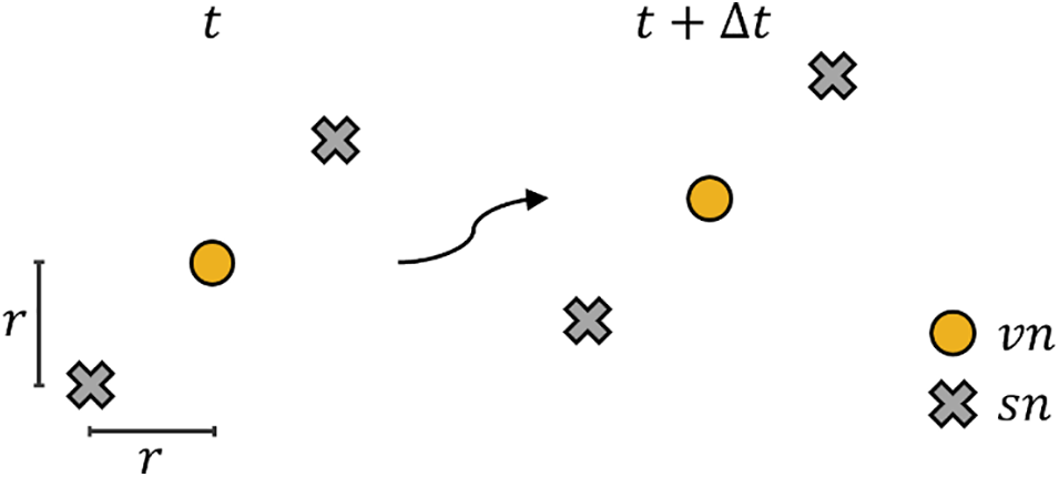
Figure 1: Stress particle SPH discretisation (modified after [46])
In the above equations,
The approximation for the acceleration due to pressure gradient (i.e., the second term on the right-hand side of Eq. (6)) ensures symmetry of interaction between a particle pair. However, Eq. (6) may result in an incorrect uplift force on particles near the soil free surface. The numerical instability is particularly significant for scenarios where ponded water is present over the soil free surface (e.g., along the upstream face of an earth dam). The uplift occurs as Eq. (6) fails to incorporate the weight of water overlying the soil free surface due to kernel truncation issue [57]. Bui et al. [57] modified the pressure gradient approximation to achieve a vanishing gradient of a constant pressure field. However, such an approximation does not yield a symmetric particle interaction. In the present study, the first-order consistent gradient approximation [58,59] is adopted wherein the gradient of the field variable
where the summation is performed over the velocity nodes,
where if
The numerical model for a typical soil slope is shown in Fig. 2a. For the analysis under static loading conditions, the boundary regions are modeled using several layers of fixed boundary particles to avoid kernel truncation for the domain particles (Fig. 2b). Virtual nodes (
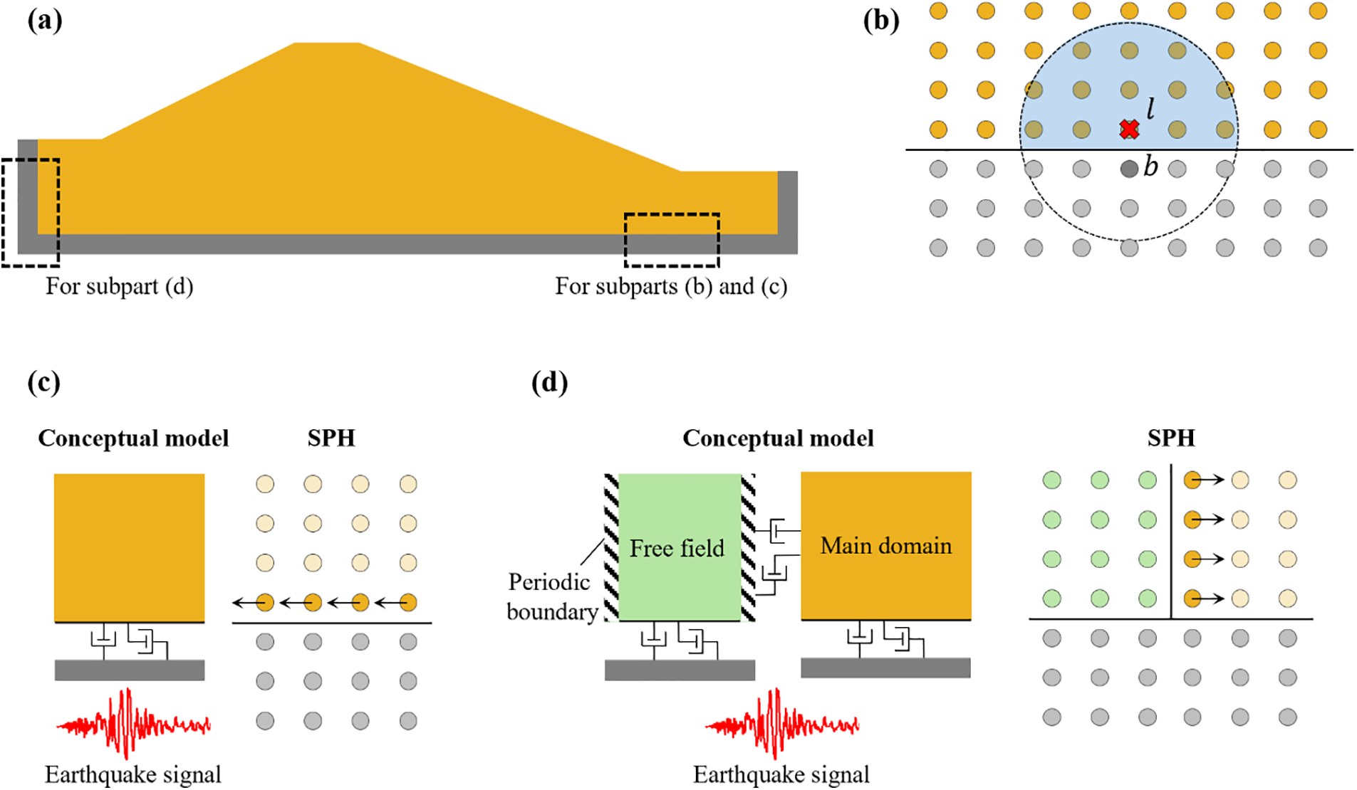
Figure 2: Boundary conditions (a) typical soil slope, (b) static analysis, (c) compliant base boundary, (d) free field boundary for seismic analysis
Hydraulic boundary conditions specifying the pressure (
As described in the Introduction, boundaries with non-reflecting (absorbing) characteristics are essential for the seismic analysis of semi-infinite domains. Chan et al. [13] described a compliant base boundary condition, wherein the earthquake ground motion is applied to the soil domain as traction time history imposed by the upward propagating stress waves. Further, the downward propagating stress waves are absorbed by viscous dashpots attached to the boundaries in the normal and shear directions [62] (Fig. 2c). The dashpot coefficients are selected to achieve an impedance ratio of one, such that no wave reflection occurs at the boundary [1,13]. In the present study, the compliant base boundary condition is adapted for SPH analysis by applyinsg the acceleration due to ground motion and viscous dashpots to the outermost layer of domain velocity nodes (Fig. 2c) as follows:
where
On the other hand, soil regions beyond the lateral boundaries exhibit free field motion under the action of seismic loading as these regions are far away from any geotechnical structure. Thus, in addition to the non-reflecting (absorbing) characteristics, the lateral boundaries (i) apply tractions on the main domain due to their motion relative to the main domain and (ii) allow the main domain to sway laterally under the effect of the earthquake. In the SPH framework, the fixed lateral boundary particles used during the static analysis are replaced by free field columns (Fig. 2d). The seismic response of the free field columns is analysed independently of the main domain by using periodic boundaries in the lateral direction with ground motion applied by the compliant base boundary condition. In mesh-based methods, the tractions due to the free field motion are applied directly on the nodes of the main domain present near the lateral boundaries [12,13,33]. However, such an approach in SPH was observed to result in stress oscillation near the lateral boundaries due to kernel truncation of the main domain particles. As a result, the approach proposed in the present study is to allow the main domain particles to interact with the free field particles inside their kernel support radius, but not vice-versa, i.e., the free field motion is not influenced by the main domain. Additionally, to model the absorbing boundary conditions, viscous dashpots are applied to the outermost layer of main domain velocity nodes (Fig. 2d) using the relative velocity of the main domain and free field,
where
The numerical implementation of the standard periodic boundary condition and modification required for accurately imposing free field conditions is detailed below. Periodic boundary conditions are modelled by allowing the interaction between particles present on opposite ends of the simulation domain. Further, a particle that leaves the simulation domain from one end is inserted from the opposite end [63]. Although such a boundary is sufficient for modelling the infinite extent of a soil domain, it fails to capture the lateral sway of the soil column under seismic loading. Consequently, the free field particles may overlap with the main domain particles, resulting in inaccurate computations or numerical instability. As a result, in addition to their true coordinates, virtual coordinates are also maintained for the free field particles during the simulation. The virtual coordinates are obtained by advancing the free field particle positions without imposing the periodicity condition, allowing the lateral sway to be modelled. Subsequently, the virtual coordinates are utilised during interaction with the main domain, whereas the free field motion is solved using the true coordinates. The modification to periodic boundary conditions for interaction between the free field and main domain allows accurate and stable imposition of free field conditions, as illustrated in Section 6.
The numerical framework described in Sections 3 and 4 is implemented in an in-house SPH code developed using the Julia programming language [56,64,65]. Further, local, non-viscous damping [66] is added to the momentum conservation equation (Eq. (6)) during the application of cyclic loading to suppress spurious particle oscillations. The acceleration due to local damping (
where
6.1 Cyclic Direct Simple Shear Test
The implementation of constitutive models in numerical frameworks designed for liquefaction hazard assessment is generally verified by the simulation of laboratory tests involving predefined stress paths and boundary conditions [51]. This ensures that the numerical framework can accurately capture the material response under controlled cyclic loading before being utilized for the analysis of more complex initial boundary value problems involving earthquake ground motion. As PM4Sand is a two-dimensional (plane-strain) model, the implementation of the PM4Sand model is verified by simulating the constant volume (undrained) cyclic direct simple shear (DSS) test. For this purpose, the results obtained from the SPH framework are compared to the benchmark results from the well-established finite element package OpenSees [68].
The numerical models are shown in Fig. 3. The SPH model (Fig. 3a) consists of a central region
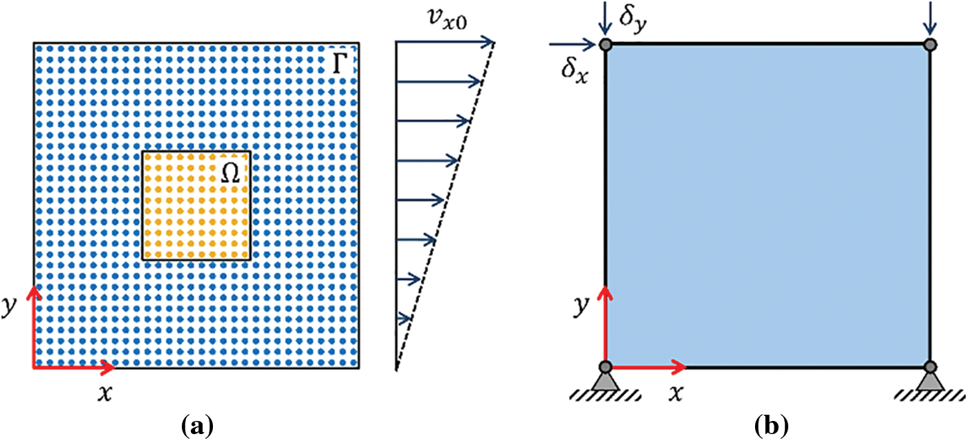
Figure 3: Cyclic direct simple shear configuration during shearing phase (a) SPH, and (b) FEM
The numerical analysis is performed for three initial states of the soil specified by the corrected SPT value
where
The numerical analysis results are illustrated in Figs. 4 to 6 in terms of the effective stress paths and stress-strain behaviour. The vertical effective stress decreases with the application of cyclic shear stress, ultimately resulting in soil liquefaction (i.e.,
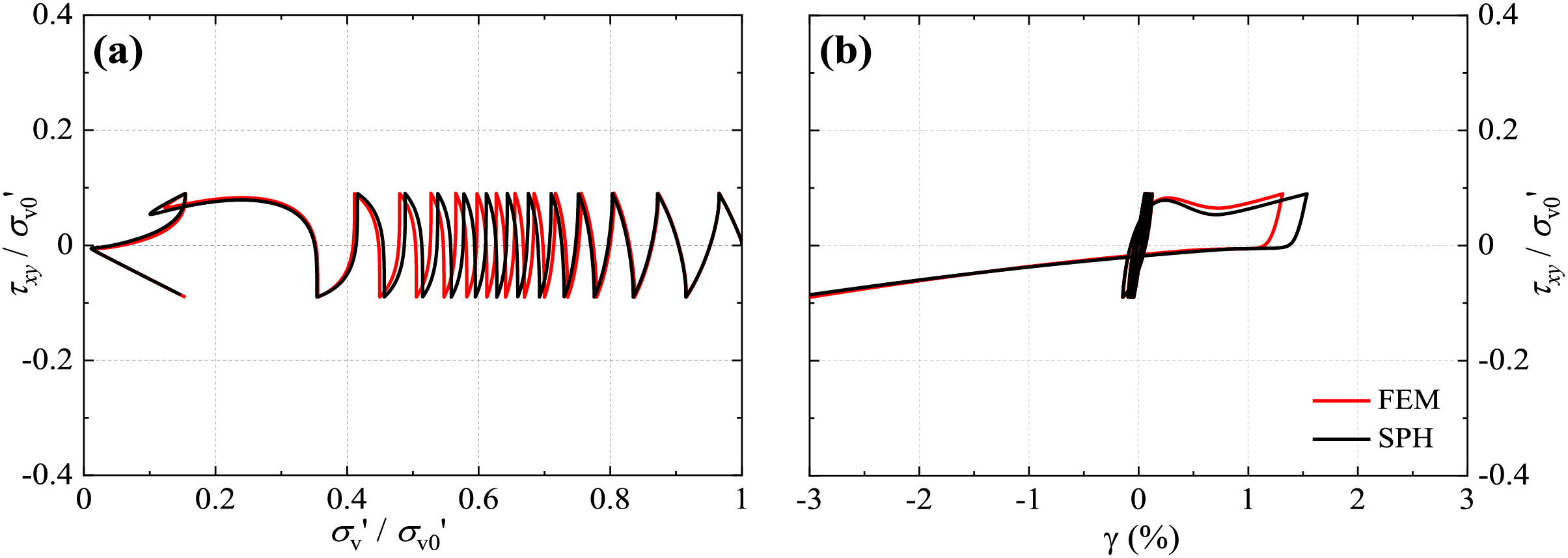
Figure 4: Cyclic direct simple shear at
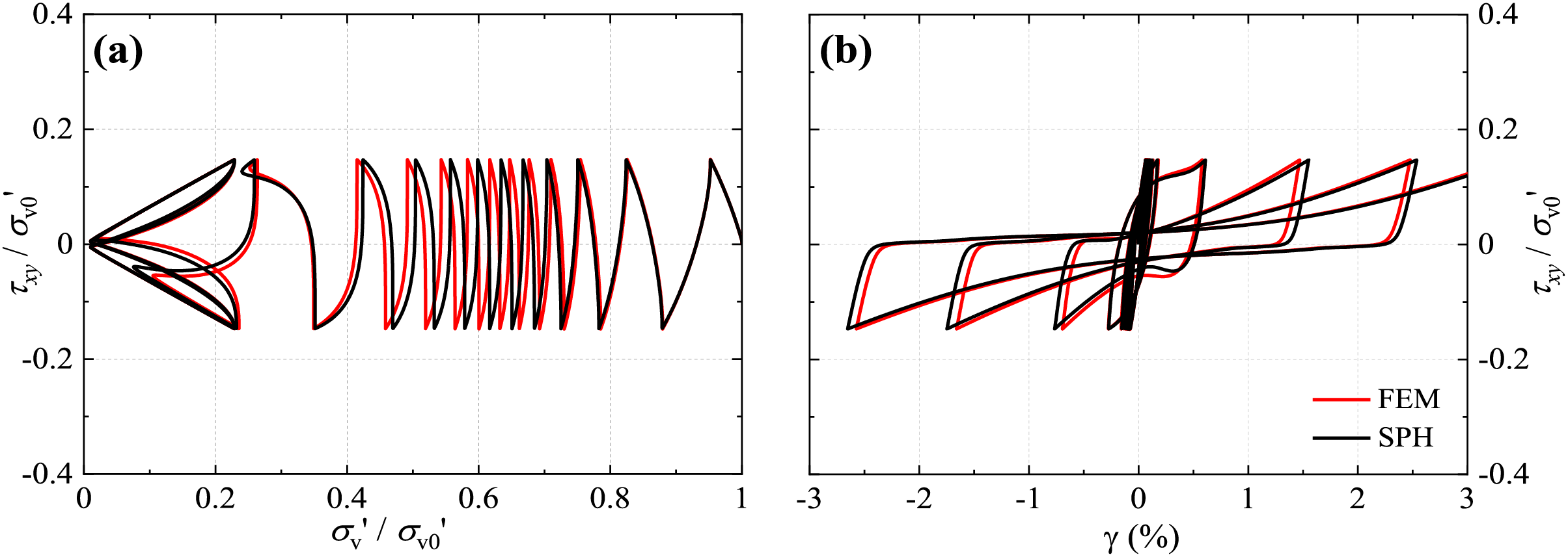
Figure 5: Cyclic direct simple shear at
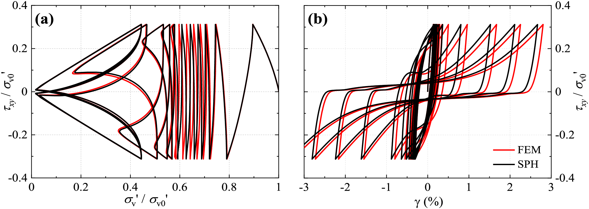
Figure 6: Cyclic direct simple shear at
6.2 Seismic Analysis of Level Ground Site
Following the verification of the PM4Sand model implementation in the previous section, the SPH framework is now adopted to analyze a more generalized scenario representative of actual field conditions. Specifically, the seismic response analysis of a level ground site comprising a layered soil deposit is carried out using the proposed SPH framework and compared with benchmark results from OpenSees [68]. The site conditions, SPH, and FEM models are shown in Fig. 7. The site consists of three soil layers with SPT
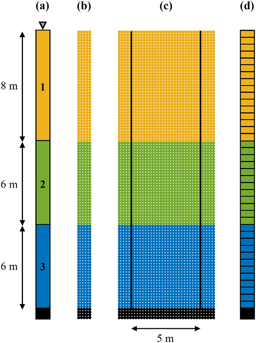
Figure 7: Seismic analysis of level ground site (a) site conditions, (b) SPH model A, (c) SPH model B, and (d) FEM model
Two SPH models, SPH A (Fig. 7b) and SPH B (Fig. 7c), are utilised for the analysis. In SPH A, a 1 m wide soil column, along with periodic boundary conditions, is used for modeling an infinitely wide, horizontal soil domain. SPH B consists of a 5 m wide main domain region, along with lateral boundary regions of 1 m width on either side. The boundary regions act as fixed support and free field columns during the static and seismic analysis, respectively (Section 4). Thus, SPH A and B differ only in terms of the lateral boundary conditions. The periodic boundaries in SPH A approximate an infinitely wide, horizontal soil domain without the requirement of any lateral boundaries, allowing the validation of the compliant base boundary condition. Subsequently, SPH B is utilized for validating the free field boundary condition by comparing the response to SPH A and FEM results. It is noteworthy that, as the main domain region in SPH B does not contain any secondary structure (e.g., earth dam), the response of SPH A and B to seismic loading is expected to be similar.
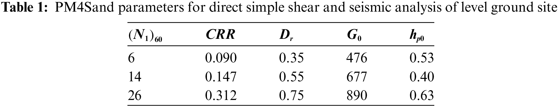
The primary calibration parameters for the PM4Sand model used in the SPH and FEM analyses are summarised in Table 1. Further, the specific gravity of soil solids
The initial effective stress state is generated using the gravity loading method in both SPH and FEM analysis. During the gravity loading phase, the Poisson’s ratio
The soil columns are subjected to the earthquake signal shown in Fig. 8. The acceleration history (Fig. 8a) is the horizontal component of the signal RSN765 recorded at Gilroy Array #1 during the 1989 Loma Prieta earthquake and has a peak acceleration of 0.47 g. The velocity history (Fig. 8b) is obtained by integrating the acceleration signal and represents the outcrop motion. Thus, the input to the SPH model (Eq. (14)) is half of the
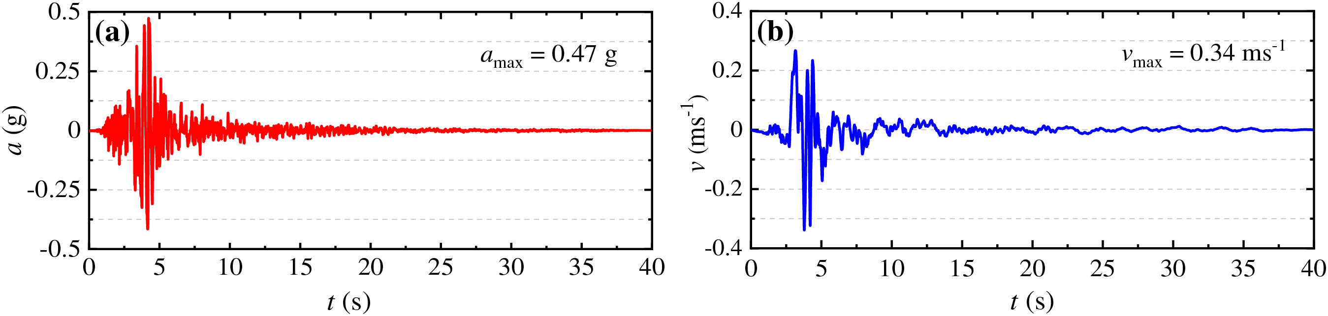
Figure 8: Input signal for seismic analysis of level ground site (a) acceleration, (b) velocity-time histories
The horizontal component of the free-surface acceleration and the corresponding response spectrum at a 5% damping ratio for the SPH and FEM analysis is shown in Fig. 9a,b, respectively. The free-surface acceleration in SPH is calculated using the interpolation equation Eq. (10). The peak acceleration from the three numerical models are 0.145 g (SPH A), 0.148 g (SPH B), and 0.150 g (FEM). Thus, the SPH analyses capture the peak and frequency content of the surface acceleration with satisfactory accuracy. The discrepancies in the SPH and FEM results may be attributed to the difference in the numerical discretization of the coupled flow-deformation model and the nature of the temporal integration scheme (i.e., explicit leapfrog method in SPH and implicit Newmark method in FEM). Nevertheless, the SPH framework satisfactorily captures the essential information necessary for engineering analysis and design.
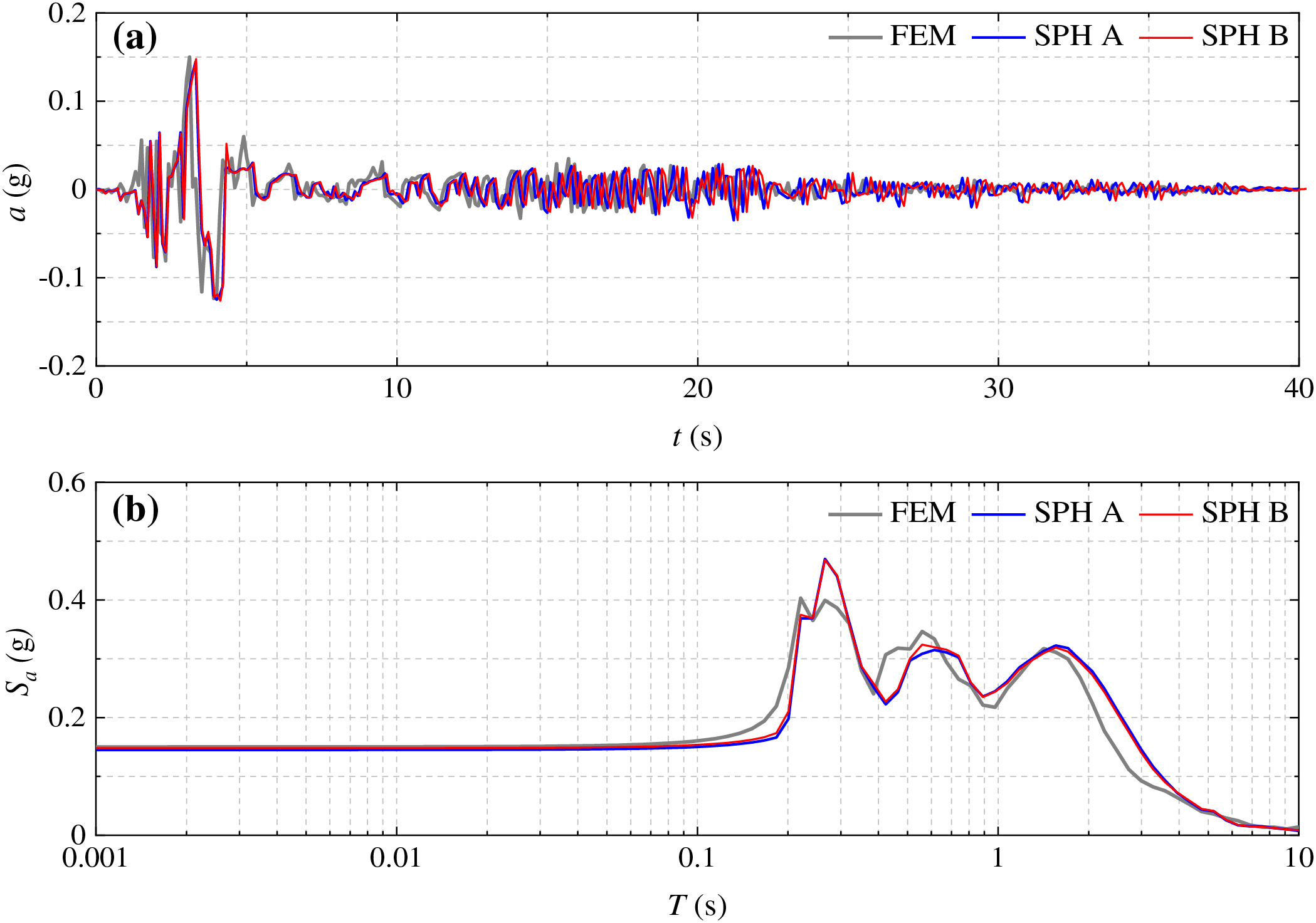
Figure 9: (a) Horizontal acceleration-time history at the free surface and (b) response spectrum at 5% damping ratio
The development of excess pore-water pressure ratio
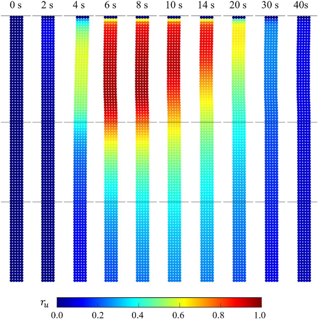
Figure 10: Excess pore-water pressure ratio (
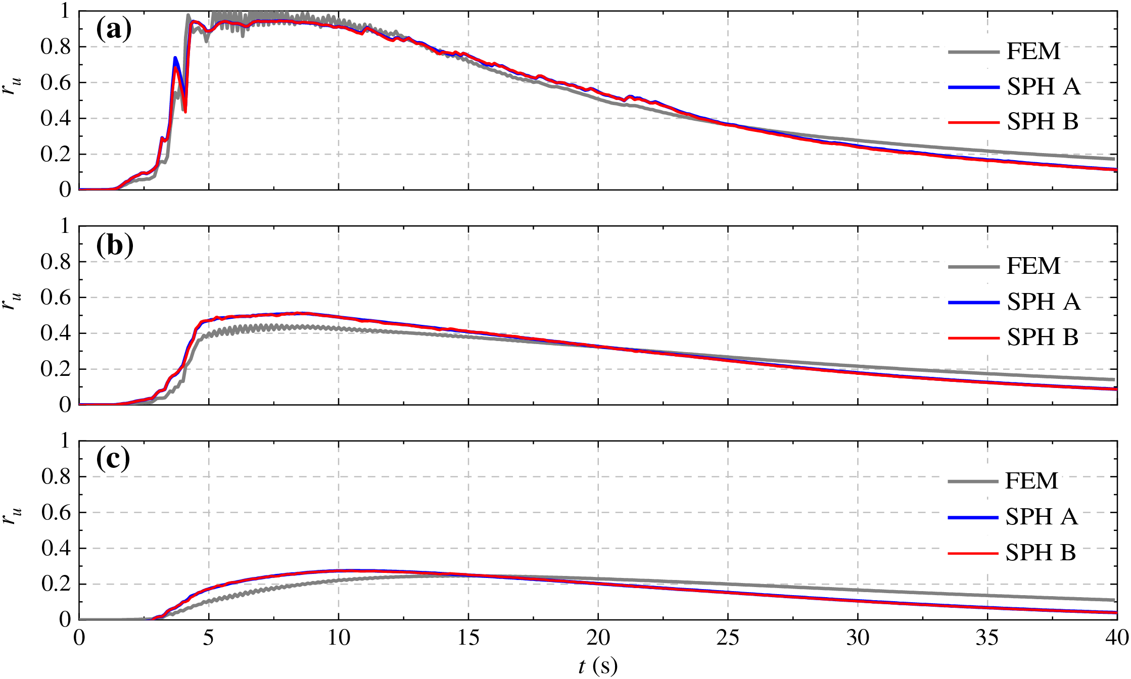
Figure 11: Excess pore-water pressure ratio (
The modification to the periodic boundary conditions proposed in Section 4 allows the lateral sway of the soil column to be observed during seismic loading (Fig. 10). The soil column demonstrates level ground liquefaction where ground oscillation is produced during the earthquake; however, the residual lateral deformation at the end of ground motion is small [1]. The response of FEM, SPH A and B in terms of the surface acceleration and development of excess pore-water pressure are almost identical, thus validating the compliant base and free field boundary conditions proposed in Section 4. The results of the seismic analysis of the level ground site demonstrate that the SPH framework is capable of modeling soil liquefaction for practical geotechnical engineering scenarios.
6.3 Liquefaction-Induced Failure of the Lower San Fernando Dam
A seismic response analysis of the Lower San Fernando Dam (LSFD) is carried out in this section to demonstrate the capability of the SPH framework to capture liquefaction-induced large deformation failures of complex geotechnical structures. The idealised cross-section of LSFD developed by Seed et al. [70] is illustrated in Fig. 12. The dam’s height is 44 m with upstream and downstream slopes of 1 V:2.5 H and 1 V:4 H, respectively. The earth dam was primarily constructed using the hydraulic fill method, resulting in a cohesive central clay core (CC) and a cohesionless shell (regions HFU 1 to 4 on the upstream and HFD 1 to 4 on the downstream side). Ground shale (GS) and rolled fill (RF) layers were placed to raise the dam’s height to the required level. A chimney drain and rolled fill (RF) berm were also constructed along the downstream slope to improve stability. The foundation consisted of upper alluvium (UA) and lower alluvium (LA) layers under stiff bedrock. The reservoir level was 338 m, whereas the downstream water level is assumed to be at the surface (305 m). Additional details on the construction methodology can be found in [12].
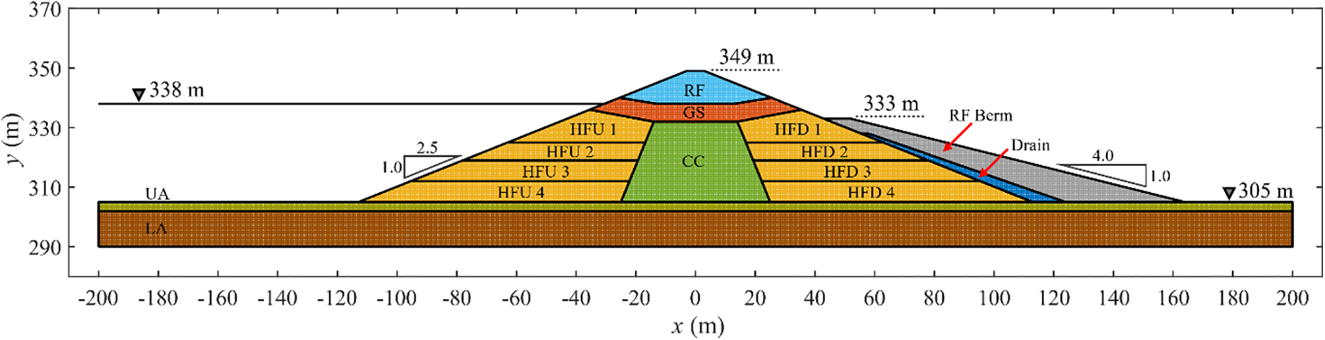
Figure 12: Geometry and initial conditions for the analysis of the Lower San Fernando Dam
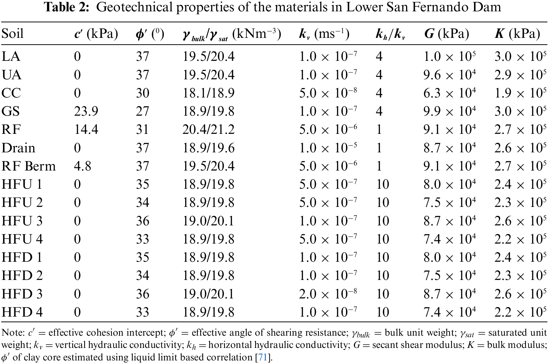
The upstream slope of the LSFD suffered a large deformation flow failure during the 1971 San Fernando Earthquake [12]. The upstream toe was displaced by 42 to 65 m into the reservoir, resulting in the settlement of the crest and almost a complete loss of the reservoir freeboard. Only minor deformations were observed on the downstream slope. Post-failure site investigation [70] identified the cause of the flow failure to be the liquefaction of the hydraulically filled shell (i.e., HFU 1 to 4 and HFD 1 to 4). Notably, liquefaction was not observed for the other soils. The geotechnical properties of the materials in LSFD are summarised in Table 2 [12].
Spatial discretisation of the numerical model is performed using approximately 20,000 particles (velocity nodes) at an initial spacing
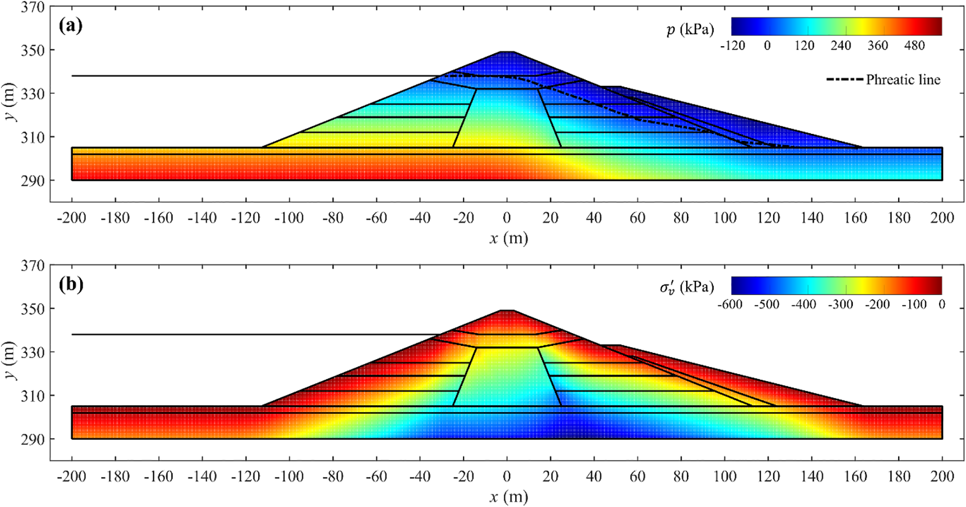
Figure 13: Pre-earthquake conditions in LSFD (a) pore-water pressure and (b) effective vertical stress
For the seismic analysis, the material model of the liquefiable soil layers (i.e., HFU 1 to 4 and HFD 1 to 4) is changed to PM4Sand. In contrast, the non-liquefiable soils are described using the Drucker Prager model. The PM4Sand model is initialised using the pre-earthquake effective stress following the procedure outlined in [51]. Chowdhury [12] utilised the finite difference package FLAC [73] for the seismic analysis of LSFD using the PM4Sand model. The PM4Sand model was calibrated to best match the post-failure field observations. In the present study, the PM4Sand calibration parameters reported by Chowdhury [12] (Table 3) are adopted for the seismic analysis to enable a straightforward comparison with the results reported in that study. Additionally, Chowdhury [12], based on a comprehensive review of the literature related to LSFD, stated that no reliable ground motion measurements were available for the LSFD site. As a result, Chowdhury [12] recommended that the acceleration-time history recorded at the nearby Pacoima dam (RSN77 in the PEER database), rotated to a direction transverse to the crest of LSFD and scaled to a peak acceleration of 0.80 g be adopted for the seismic analysis. The scaling factor was deduced based on an assessment of the expected ground motions at the LSFD site, considering the effect of local geology using the modern NGA-West2 ground motion prediction equations [67]. Further, the scaling factor was corroborated by a series of simulations of possible slip mechanism scenarios during the 1971 San Fernando earthquake. As a result, the scaled ground motion represents the best estimate of the ground motion at LSFD. A detailed discussion of various aspects related to the input ground motion for seismic analysis of LSFD can be found in [12]. In the present study, the numerical model is subjected to the ground motion shown in Fig. 14, adopted from Doan et al. [19]. The velocity history (Fig. 14b) is obtained by integrating the acceleration signal. Half of the velocity signal (Fig. 14b) is applied as input to the SPH model using Eq. (14). The base boundary condition is modified to free slip to transfer the ground motion to the numerical model accurately. Further, the fixed lateral boundaries are replaced by free field columns following the procedure outlined in Section 4. The ground motion is applied using the compliant base boundary conditions with the viscous dashpots assigned the properties of the lower alluvium, local damping coefficient
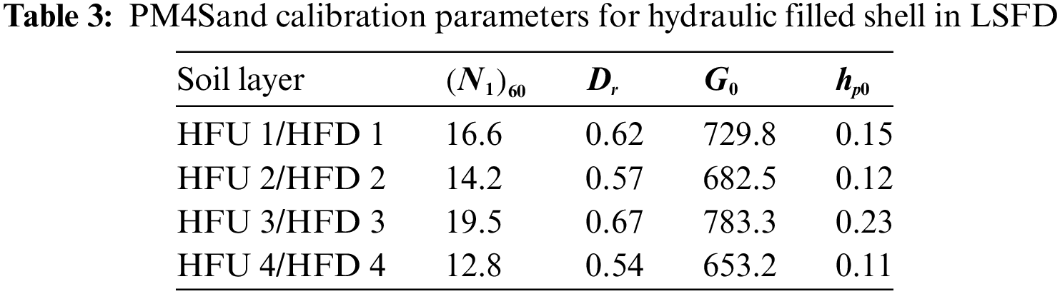
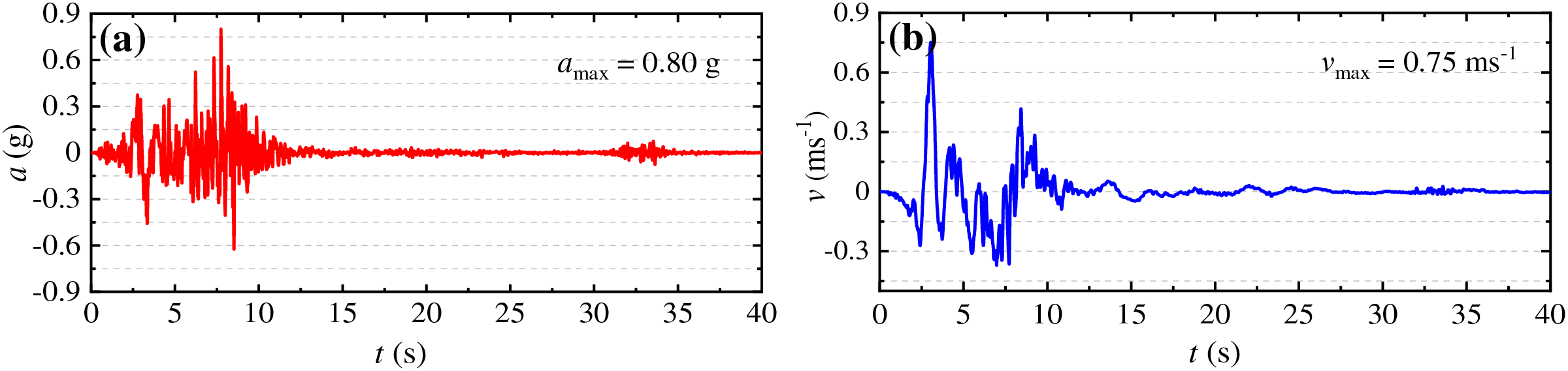
Figure 14: Input signal for seismic analysis of LSFD (a) acceleration and (b) velocity-time histories
Fig. 15a,b illustrates the maximum excess pore-water pressure ratio and shear strain in the hydraulic filled shell developed during the earthquake. The excess pore-water pressure ratio is calculated as
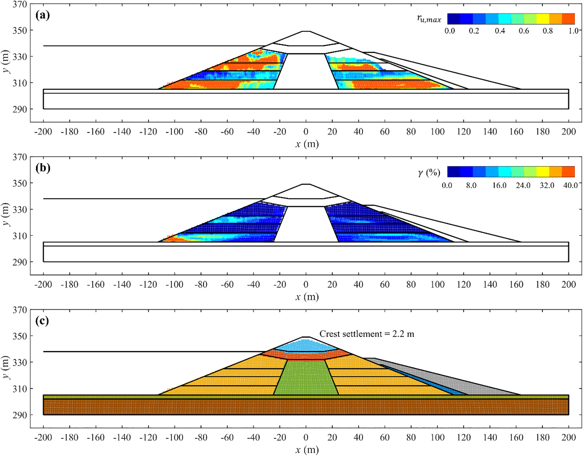
Figure 15: (a) Maximum excess pore-water pressure ratio in the hydraulic filled shell, (b) shear strain in the hydraulic filled shell, and (c) crest settlement at the end of the earthquake
The large deformation flow behaviour is governed by the shear strength of the liquefied soil. However, the PM4Sand model does not implicitly transition to the post-liquefaction residual shear strength during the application of the ground motion to the numerical model [12]. As a result, the commonly adopted approach is to identify the elements or particles that undergo liquefaction and assign post-liquefaction residual shear strength for the post-earthquake analysis. A soil element or node is considered to be liquefied if the maximum excess pore-water pressure ratio
The liquefied soil is described by an effective stress analysis using the Drucker Prager model. The
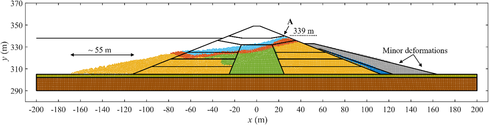
Figure 16: Final deformation profile for the Lower San Fernando Dam
Section 6 demonstrates that the proposed SPH framework can model soil liquefaction with satisfactory accuracy. The results of the SPH analysis are consistent with FEM simulations or results from published studies for liquefaction triggering. Additionally, owing to the meshless nature of the method, the post-liquefaction large deformation behaviour can also be analysed, making the framework suitable for liquefaction hazard assessment.
Numerical analysis of seismic hazards (such as liquefaction) remains a continually evolving field, driven by advancements in computational techniques and a deepening understanding of soil behaviour under cyclic loading conditions. The present study is expected to serve as the foundation for further development of SPH-based numerical techniques that contribute to safer and more resilient geotechnical structures in seismically active areas. In this regard, a few essential features of the proposed SPH framework and associated limitations that can be addressed by future studies are further elaborated in this section.
• The PM4Sand model has been developed to emulate field observations and empirical correlations for soil liquefaction commonly employed in earthquake geotechnical engineering [51]. The model has been extensively utilized in liquefaction studies due to its satisfactory performance in reproducing laboratory and field observations and the relative ease of calibration based on a few parameters that can be derived from routine geotechnical investigations. Accordingly, the present study adopts the PM4Sand model to describe the behaviour of the liquefiable soils subjected to cyclic loading.
• The PM4Sand model can be calibrated to capture a wide range of behaviours related to pore-water pressure generation and cyclic strains. Nevertheless, the present study adopts the PM4Sand calibration parameters from the literature to validate the various aspects of the proposed SPH framework by comparing the numerical results with benchmark FEM simulations or field observations reported in the published studies.
• It is noteworthy that using predefined PM4Sand calibration parameters for validation does not affect the generalizability of the various components of the proposed SPH framework (e.g., spatial discretization and boundary conditions). Accordingly, the SPH framework can be used for predictive analysis by calibrating the PM4Sand model using laboratory and field observations following the procedure described in [43,44].
• Although the PM4Sand model has been extensively adopted for liquefaction analysis, no single constitutive model can fully capture the complex behaviour of soils under all conditions. As a result, a comparison between the numerical accuracy of various constitutive models implemented within the SPH framework is essential. Although the substitution of constitutive models is straightforward due to the modular nature of the SPH framework, such an exercise is not carried out in the present study.
• Further, the PM4Sand model is only applicable for two-dimensional (plane-strain) analysis, and alternate soil models will be necessary to extend the SPH framework for three-dimensional scenarios.
7.2 Boundary Conditions & Input Ground Motion
• Non-reflecting (absorbing) boundary conditions for seismic analysis using the SPH method are proposed in Section 4. The numerical examples demonstrate that the boundary conditions can accurately transfer the ground motion and model the non-reflecting conditions. Although the focus of the present study is soil liquefaction, the boundary conditions are generalized and can also be applied for modeling (i) other seismic hazards, such as seismically induced landslides, (ii) blast-induced soil liquefaction, or (iii) dynamic soil-structure interaction problems in semi-infinite or infinite soil domains.
• The earthquake ground motion is imposed as a traction time history based on the principles of stress wave propagation in elastic media (Eqs. (14) and (15)). Thus, the artificial boundaries should be sufficiently far away from the region of major deformations to ensure low strain levels at the boundary.
• The ground motion signal is applied uniformly over the compliant base boundary in the form of vertically propagating stress waves. In reality, such a condition can only be assumed after the seismic waves have traveled a considerable distance from the earthquake source and have been subjected to multiple refractions [1]. As a result, applying a non-uniform ground motion signal will be essential for the analysis of sites that are relatively near the earthquake source.
• For modeling the lateral non-reflecting boundaries, the fixed boundary particles used in the static analysis are replaced by free field columns. The motion of the free field particles is solved independently using periodic boundary conditions to approximate infinitely wide, horizontal soil domains. Additionally, the free field particles interact with the main domain region (Fig. 2). As a result, the complexity of the numerical algorithm is enhanced due to the requirement of additional particle interactions. Moreover, the computational efficiency is reduced as neighbour search and particle interactions are often the most computationally expensive operations in particle-based methods.
• The modification to the periodic boundary conditions allows the lateral sway of the free field columns to be modeled. Nevertheless, some particle disorder in the main domain region near the lateral boundaries may still be observed due to the application of the viscous dashpot forces as point loads. However, the effect of particle disorder on the numerical results is expected to be minimal as the lateral boundaries are required to be sufficiently away from the regions of significant deformations to satisfy the assumption of elastic wave propagation.
• The seismic analyses in Sections 6.2 and 6.3 were carried out using representative ground motions (Figs. 8 and 14) for validating the various aspects of the SPH framework by comparing the results with FEM simulations or published studies. In general, ground motion characteristics, i.e., peak ground acceleration (PGA), frequency content, and duration of ground motion, directly influence the nonlinear seismic response of soil deposits as well as the built infrastructure on it. Specifically, (i) a higher PGA indicates a higher intensity of ground shaking and higher inertial loads, (ii) frequency content governs potential resonance scenarios, where high amplitude vibrations occur if the ground motion frequency matches the natural frequency of the structure, and (iii) a higher duration of ground motion leads to a higher excess pore-water pressure accumulation and stiffness degradation. The ground motion characteristics are dictated by the geological conditions of a site (i.e., the soil or rock type). Hence, when employing the SPH framework for predictive analysis, selecting ground motion representative of the site-specific conditions is fundamental for achieving accurate and reliable seismic response.
• Earthquake-induced ground motion is typically recorded at rock outcrops. However, for seismic analysis, the input ground motion must be specified at the level of the compliant base boundary. Accordingly, an equivalent linear deconvolution analysis of the rock outcrop motion will be necessary to obtain the appropriate input ground motion for the SPH model [1].
7.3 Validation of the SPH Framework Using Field Data
• A potential limitation of the present study is that the validation is performed using only FEM simulations or results from published studies. It is acknowledged that further validation based on field data is fundamental to establishing the SPH framework for seismic analysis of geotechnical structures. Such an exercise is being undertaken by integrating field data collected using static and seismic Cone Penetration Tests (CPTs) and Hydraulic Profiling Tool (HPT) at an earth dam site in India into the proposed SPH framework.
• Nevertheless, the comprehensive statistical validation of the framework prediction with the field measured data, as well as the sensitivity analysis to assess the numerical stability and robustness of the framework, is beyond the scope of the present study and will be reported in our future works.
7.4 Computational Expense of the SPH Framework
• The present study adopts the single-layer SPH discretization wherein the fluid phase is described in an Eulerian reference frame moving with the soil phase. Although the single-layer approach is efficient for large-scale applications [45,56], the computational expense is still significantly higher than mesh-based methods (i.e., FEM or FDM). As a result, mesh-based methods may be preferred over SPH for seismic analysis when material deformations are limited or when the post-failure large deformation behaviour is not of concern.
• For large deformation analysis, a hybrid numerical approach using mesh-based and meshless SPH methods for the pre-and post-failure analysis, respectively, can be adopted to improve the overall computational efficiency. However, the hybrid approach is not suitable for coseismic deformation scenarios wherein large deformations may be observed during the ground motion period, which is often resolved using mesh-based techniques [33].
• On the other hand, the SPH approach can effectively cater to both small and large deformation scenarios, as demonstrated by the present study. Specifically, for the seismic analysis of a level ground site (Section 6.2), the soil profile demonstrates lateral deformation during the ground motion period. However, the final displacement is small (Fig. 10). In contrast, the liquefaction-induced failure of the Lower San Fernando Dam (Section 6.3) illustrates the capability of the framework in capturing liquefaction triggering and gravity-driven mass flow involving large deformations (Fig. 16).
• Nevertheless, the computational efficiency of the algorithm and the SPH framework needs to be improved to allow large-scale or three-dimensional analysis. For this purpose, parallelization techniques based on CPUs or GPUs are available [75–79]. However, such a development is beyond the scope of the present study.
This study presents a numerical framework for the earthquake-induced liquefaction hazard assessment of geotechnical structures based on a three-phase, single-layer SPH approach, with the behaviour of soils subjected to cyclic loading described using the PM4Sand model. The spatial discretisation is carried out using the stress particle SPH method to minimise the effects of zero-energy modes and tensile instability on the numerical solution. Additionally, compliant base and free field boundary conditions appropriate for the SPH method are proposed, allowing the numerical treatment of unbounded (semi-infinite) soil domains. Numerical analysis of (i) cyclic direct simple shear test, (ii) seismic response of a level ground site, and (iii) liquefaction-induced failure of the Lower San Fernando Dam is carried out to demonstrate that the SPH framework can model the liquefaction triggering, as well as the post-liquefaction large deformation behaviour with satisfactory accuracy. Although the present study is primarily targeted toward soil liquefaction, the proposed SPH framework is versatile and can be adapted for modeling other scenarios of soil subjected to cyclic loading (e.g., seismically induced landslides). Such applications will be explored in future studies to enhance the understanding and management of seismic hazards.
Acknowledgement: This research did not receive any specific grant from funding agencies in the public, commercial, or not-for-profit sectors. This study is inspired by an extensive association (from investigation stage onwards) in the analysis and design of the Main Dam of Polavaram Irrigation Project, India through several agencies such as the Water Resources Department, Andhra Pradesh, India; Megha Engineering and Infrastructure Limited; Navayuga Engineering Company. The insights gained through these works, particularly from projects IITD/IRD/CW14168, CW14469, and CW14378, have significantly contributed to the development of the analysis presented in this study.
Funding Statement: The authors received no specific funding for this study.
Author Contributions: The authors confirm their contribution to the paper as follows: study conception and design: Sourabh Mhaski, G. V. Ramana; analysis and interpretation of results: Sourabh Mhaski, G. V. Ramana; draft manuscript preparation: Sourabh Mhaski; review & editing: G. V. Ramana. All authors reviewed the results and approved the final version of the manuscript.
Availability of Data and Materials: Data sharing is not applicable to this article as no datasets were generated or analysed during the current study.
Ethics Approval: Not applicable.
Conflicts of Interest: The authors declare no conflicts of interest to report regarding the present study.
References
1. Kramer SL. Geotechnical earthquake engineering. Upper Saddle River, New Jersey, USA: Prentice-Hall; 1996. [Google Scholar]
2. Xu C, Ma S, Tan Z, Xie C, Toda S, Huang X. Landslides triggered by the 2016 Mj 7.3 Kumamoto, Japan, earthquake. Landslides. 2018;15(3):551–64. doi:10.1007/s10346-017-0929-1. [Google Scholar] [CrossRef]
3. Bhattacharya S, Hyodo M, Nikitas G, Ismael B, Suzuki H, Lombardi D, et al. Geotechnical and infrastructural damage due to the 2016 Kumamoto earthquake sequence. Soil Dyn Earthq Eng. 2018;104(1):390–4. doi:10.1016/j.soildyn.2017.11.009. [Google Scholar] [CrossRef]
4. Bhattacharya S, Hyodo M, Goda K, Tazoh T, Taylor CA. Liquefaction of soil in the Tokyo Bay area from the 2011 Tohoku (Japan) earthquake. Soil Dyn Earthq Eng. 2011;31(11):1618–28. doi:10.1016/j.soildyn.2011.06.006. [Google Scholar] [CrossRef]
5. Bray JD, Markham CS, Cubrinovski M. Liquefaction assessments at shallow foundation building sites in the central business district of christchurch, New Zealand. Soil Dyn Earthq Eng. 2017;92(4):153–64. doi:10.1016/j.soildyn.2016.09.049. [Google Scholar] [CrossRef]
6. Sonmez B, Ulusay R, Sonmez H. A study on the identification of liquefaction-induced failures on ground surface based on the data from the 1999 Kocaeli and Chi-Chi earthquakes. Eng Geol. 2008;97(3–4):112–25. doi:10.1016/j.enggeo.2007.12.008. [Google Scholar] [CrossRef]
7. Yoshida N, Watanabe H, Yasuda S, Mora Castro S. Liquefaction-induced ground failure and related damage to structures during 1991 Telire-Limon, Costa Rica, earthquake. In: Proceedings from the Fourth Japan-US Workshop on Earthquake Resistant Design of Lifeline Facilities and Countermeasures for Soil Liquefaction, 1992; HI, USA: p. 37–52. [Google Scholar]
8. Seed RB, Dickenson SE, Idriss IM. Principal geotechnical aspects of the 1989 Loma Prieta earthquake. Soils Found. 1991;31(1):1–26. doi:10.3208/sandf1972.31.1. [Google Scholar] [CrossRef]
9. Soga K. Soil liquefaction effects observed in the Kobe earthquake of 1995. Proc Inst Civ Eng Geotech Eng., 1998;131(1):34–51. doi:10.1061/JSFEAQ.0001260. [Google Scholar] [CrossRef]
10. Seed HB, Idriss IM. Influence of soil conditions on ground motions during earthquakes. J Soil Mech Found Div. 1969;95(1):99–137. doi:10.1061/JSFEAQ.0001260. [Google Scholar] [CrossRef]
11. Elia G, Rouainia M. Advanced dynamic nonlinear schemes for geotechnical earthquake engineering applications: a review of critical aspects. Geotech Geol Eng. 2022;40(7):3379–92. doi:10.1007/s10706-022-02109-6. [Google Scholar] [CrossRef]
12. Chowdhury KH. Evaluation of the state of practice regarding nonlinear seismic deformation analyses of embankment dams subject to soil liquefaction based on case histories (Ph.D. Thesis). University of California: Berkeley; 2018. [Google Scholar]
13. Chan AHC, Pastor M, Schrefler BA, Shiomi T, Zienkiewicz OC. Computational geomechanics: theory and applications. Hoboken, NJ, USA: John Wiley & Sons; 2022. [Google Scholar]
14. Cui CY. Seismic behavior and reinforcement mechanisms of earth dam and liquefiable foundation system by shaking table tests and numerical simulation. Soil Dyn Earthq Eng. 2023;173(5):108083. doi:10.1016/j.soildyn.2023.108083. [Google Scholar] [CrossRef]
15. Li G, Motamed R. Finite element modeling of soil-pile response subjected to liquefaction-induced lateral spreading in a large-scale shake table experiment. Soil Dyn Earthq Eng. 2017;92(3):573–84. doi:10.1016/j.soildyn.2016.11.001. [Google Scholar] [CrossRef]
16. Kang GC, Tobita T, Iai S. Seismic simulation of liquefaction-induced uplift behavior of a hollow cylinder structure buried in shallow ground. Soil Dyn Earthq Eng. 2014;64(1):85–94. doi:10.1016/j.soildyn.2014.05.006. [Google Scholar] [CrossRef]
17. Tang XW, Zhang XW, Uzuoka R. Novel adaptive time stepping method and its application to soil seismic liquefaction analysis. Soil Dyn Earthq Eng. 2015;71(9):100–13. doi:10.1016/j.soildyn.2015.01.016. [Google Scholar] [CrossRef]
18. Qiu Z, Lu J, Elgamal A, Su L, Wang N, Almutairi A. OpenSees three-dimensional computational modeling of ground structure systems and liquefaction scenarios. Comput Model Eng Sci. 2019;120(3):629–56. doi:10.32604/cmes.2019.05759. [Google Scholar] [CrossRef]
19. Doan NP, Nguyen BP, Park SS. Seismic deformation analysis of earth dams subject to liquefaction using UBCSAND2 model. Soil Dyn Earthq Eng. 2023;172:108003. doi:10.1016/j.soildyn.2023.108003. [Google Scholar] [CrossRef]
20. Boulanger RW, Montgomery J. Nonlinear deformation analyses of an embankment dam on a spatially variable liquefiable deposit. Soil Dyn Earthq Eng. 2016;91(3):222–33. doi:10.1016/j.soildyn.2016.07.027. [Google Scholar] [CrossRef]
21. Liu Y, Chen X, Hu M. Three-dimensional large deformation modeling of landslides in spatially variable and strain-softening soils subjected to seismic loads. Can Geotech J. 2023;60(4):426–37. [Google Scholar]
22. Liu S, Tang X, Li J. A decoupled Arbitrary Lagrangian-Eulerian method for large deformation analysis of saturated sand. Soils Found. 2022;62(2):101110. doi:10.1016/j.sandf.2022.101110. [Google Scholar] [CrossRef]
23. Zhuang H, Hu Z, Wang X, Chen G. Seismic responses of a large underground structure in liquefied soils by FEM numerical modelling. Bull Earthq Eng. 2015;13(12):3645–68. [Google Scholar]
24. Liang W, Zhao J, Wu H, Soga K. Multiscale, multiphysics modeling of saturated granular materials in large deformation. Comput Methods Appl Mech Eng. 2023;405:115871. doi:10.1016/j.cma.2022.115871. [Google Scholar] [CrossRef]
25. Qin J, Mei G, Xu N. Meshfree methods in geohazards prevention: a survey. Arch Comput Methods Eng. 2022;29(5):3151–82. doi:10.1007/s11831-021-09686-4. [Google Scholar] [CrossRef]
26. Bui HH, Nguyen GD. Smoothed particle hydrodynamics (SPH) and its applications in geomechanics: from solid fracture to granular behaviour and multiphase flows in porous media. Comput Geotech. 2021;138(5):104315. doi:10.1016/j.compgeo.2021.104315. [Google Scholar] [CrossRef]
27. Soga K, Alonso E, Yerro A, Kumar K, Bandara S, Kwan JSH, et al. Trends in large-deformation analysis of landslide mass movements with particular emphasis on the material point method. Geotechnique. 2018;68(5):457–8. doi:10.1680/jgeot.15.LM.005. [Google Scholar] [CrossRef]
28. Sizkow SF, El Shamy U. SPH-DEM modeling of the seismic response of shallow foundations resting on liquefiable sand. Soil Dyn Earthq Eng. 2022;156(3):107210. doi:10.1016/j.soildyn.2022.107210. [Google Scholar] [CrossRef]
29. Sizkow SF, El Shamy U. SPH-DEM simulations of saturated granular soils liquefaction incorporating particles of irregular shape. Comput Geotech. 2021;134(3):104060. doi:10.1016/j.compgeo.2021.104060. [Google Scholar] [CrossRef]
30. El Shamy U, Sizkow SF. Coupled SPH-DEM simulations of liquefaction-induced flow failure. Soil Dyn Earthq Eng. 2021;144(3):106683. doi:10.1016/j.soildyn.2021.106683. [Google Scholar] [CrossRef]
31. Talbot LED, Given J, Tjung EYS, Liang Y, Chowdhury K, Seed R, et al. Modeling large-deformation features of the Lower San Fernando Dam failure with the material point method. Comput Geotech. 2024;165(2):105881. doi:10.1016/j.compgeo.2023.105881. [Google Scholar] [CrossRef]
32. Zai D, Pang R, Xu B, Liu J. Seismic failure probability analysis of slopes via stochastic material point method. Soil Dyn Earthq Eng. 2023;172(2):108041. doi:10.1016/j.soildyn.2023.108041. [Google Scholar] [CrossRef]
33. Kohler M, Stoecklin A, Puzrin AM. A MPM framework for large-deformation seismic response analysis. Can Geotech J. 2022;59(6):1046–60. doi:10.1139/cgj-2021-0252. [Google Scholar] [CrossRef]
34. Kohler M, Puzrin AM. Mechanism of Co-Seismic deformation of the slow-moving la sorbella landslide in italy revealed by MPM analysis. J Geophys Res Earth Surf. 2022;127(7):1–25. doi:10.1029/2022JF006618. [Google Scholar] [CrossRef]
35. Giridharan S, Gowda S, Stolle DFE, Moormann C. Comparison of UBCSAND and hypoplastic soil model predictions using the material point method. Soils Found. 2020;60(4):989–1000. doi:10.1016/j.sandf.2020.06.001. [Google Scholar] [CrossRef]
36. Mao Z, Liu G, Huang Y, Bao Y. A conservative and consistent Lagrangian gradient smoothing method for earthquake-induced landslide simulation. Eng Geol. 2019;260(9):105226. doi:10.1016/j.enggeo.2019.105226. [Google Scholar] [CrossRef]
37. Chen W, Qiu T. Simulation of earthquake-induced slope deformation using SPH method. Int J Numer Anal Methods Geomech. 2014;38(3):297–330. [Google Scholar]
38. Bui HH, Fukagawa R, Sako K, Okamura Y. Earthquake induced slope failure simulation by SPH. In: International Conference on Recent Advances in Geotechnical Earthquake Engineering and Soil Dynamics, 2010; San Diego, CA, USA. [Google Scholar]
39. Shuai H, Liu CZ, Katsuichiro G. Applicability of smooth particle hydrodynamics method to large sliding deformation of saturated slopes under earthquake action. Chinese J Geotech Eng. 2023;45(2):336–44 (In Chinese). [Google Scholar]
40. Bao Y, Huang Y, Liu GR, Wang G. SPH simulation of high-volume rapid landslides triggered by earthquakes based on a unified constitutive Model. Part I: initiation process and slope failure. Int J Comput Methods. 2020;17(4):1850150. doi:10.1142/S0219876218501505. [Google Scholar] [CrossRef]
41. Zhang W, Yu R, Chen Y, Chen S. SPH analysis of sliding material volume and influence range of soil slope under earthquake. Front Phys. 2022;10:1–9. [Google Scholar]
42. Huang Y, Li G, Xiong M. Stochastic assessment of slope failure run-out triggered by earthquake ground motion. Nat Hazards. 2020;101(1):87–102. doi:10.1007/s11069-020-03863-7. [Google Scholar] [CrossRef]
43. Boulanger RW, Ziotopoulou K. Formulation of a sand plasticity plane-strain model for earthquake engineering applications. Soil Dyn Earthq Eng. 2013;53(6):254–67. doi:10.1016/j.soildyn.2013.07.006. [Google Scholar] [CrossRef]
44. Ziotopoulou K, Boulanger RW. Plasticity modeling of liquefaction effects under sloping ground and irregular cyclic loading conditions. Soil Dyn Earthq Eng. 2016;84(1):269–83. doi:10.1016/j.soildyn.2016.02.013. [Google Scholar] [CrossRef]
45. Lian Y, Bui HH, Nguyen GD, Zhao S, Haque A. A computationally efficient SPH framework for unsaturated soils and its application to predicting the entire rainfall-induced slope failure process. Geotechnique. 2022;74(8):787–805. [Google Scholar]
46. Chalk CM, Pastor M, Peakall J, Borman DJ, Sleigh PA, Murphy W, et al. Stress-particle smoothed particle hydrodynamics: an application to the failure and post-failure behaviour of slopes. Comput Methods Appl Mech Eng. 2020;366(1):113034. doi:10.1016/j.cma.2020.113034. [Google Scholar] [CrossRef]
47. Randles PW, Libersky LD. Normalized SPH with stress points. Int J Numer Methods Eng. 2000;48(10):1445–62. doi:10.1002/1097-0207(20000810)48:10<1445::AID-NME831>3.0.CO;2-9. [Google Scholar] [CrossRef]
48. Lian Y, Bui HH, Nguyen GD, Tran HT, Haque A. A general SPH framework for transient seepage flows through unsaturated porous media considering anisotropic diffusion. Comput Methods Appl Mech Eng. 2021;387:114169. doi:10.1016/j.cma.2021.114169. [Google Scholar] [CrossRef]
49. Dafalias YF, Manzari MT. Simple plasticity sand model accounting for fabric change effects. J Eng Mech. 2004;130(6):622–34. doi:10.1061/(ASCE)0733-9399(2004)130:6(622). [Google Scholar] [CrossRef]
50. Manzari MT, Dafalias YF. A critical state two-surface plasticity model for sands. Géotechnique. 1997;47(2):255–72. doi:10.1680/geot.1997.47.2.255. [Google Scholar] [CrossRef]
51. Chen L, Arduino P. Implementation, verification, and validation of the PM4Sand model in OpenSees. Berkeley: University of California, Pacific Earthquake Engineering Research Center; PEER Report No. 2021/02. doi: 10.55461/SJEU6160. [Google Scholar] [CrossRef]
52. Dinesh N, Banerjee S, Rajagopal K. Performance evaluation of PM4Sand model for simulation of the liquefaction remedial measures for embankment. Soil Dyn Earthq Eng. 2022;152(5):107042. doi:10.1016/j.soildyn.2021.107042. [Google Scholar] [CrossRef]
53. Bui HH, Fukagawa R, Sako K, Ohno S. Lagrangian meshfree particles method (SPH) for large deformation and failure flows of geomaterial using elastic-plastic soil constitutive model. Int J Numer Anal Methods Geomech. 2008 Aug 25;32(12):1537–70. doi:10.1002/nag.688. [Google Scholar] [CrossRef]
54. Monaghan JJ. Smoothed particle hydrodynamics and its diverse applications. Annu Rev Fluid Mech. 2011;44:323–46. [Google Scholar]
55. Violeau D, Rogers BD. Smoothed particle hydrodynamics (SPH) for free-surface flows: past, present and future. J Hydraul Res. 2016;54(1):1–26. doi:10.1080/00221686.2015.1119209. [Google Scholar] [CrossRef]
56. Mhaski S, Ramana GV. Modelling coupled flow-solute transport in porous media using smoothed particle hydrodynamics (SPH). Comput Geotech. 2024;167:106097. doi:10.1016/j.compgeo.2024.106097. [Google Scholar] [CrossRef]
57. Bui HH, Fukagawa R. An improved SPH method for saturated soils and its application to investigate the mechanisms of embankment failure: case of hydrostatic pore-water pressure. Int J Numer Anal Methods Geomech. 2013 Jan 1;37(1):31–50. doi:10.1002/nag.1084. [Google Scholar] [CrossRef]
58. Feng R, Fourtakas G, Rogers BD, Lombardi D. A general smoothed particle hydrodynamics (SPH) formulation for coupled liquid flow and solid deformation in porous media. Comput Methods Appl Mech Eng. 2024;419(5):116581. doi:10.1016/j.cma.2023.116581. [Google Scholar] [CrossRef]
59. Liu MB, Liu GR. Restoring particle consistency in smoothed particle hydrodynamics. Appl Numer Math. 2006;56(1):19–36. doi:10.1016/j.apnum.2005.02.012. [Google Scholar] [CrossRef]
60. Marrone S, Antuono M, Colagrossi A, Colicchio G, Le Touzé D, Graziani G. δ-SPH model for simulating violent impact flows. Comput Methods Appl Mech Eng. 2011;200(13–16):1526–42. doi:10.1016/j.cma.2010.12.016. [Google Scholar] [CrossRef]
61. English A, Domínguez JM, Vacondio R, Crespo AJC, Stansby PK, Lind SJ, et al. Modified dynamic boundary conditions (mDBC) for general-purpose smoothed particle hydrodynamics (SPHapplication to tank sloshing, dam break and fish pass problems. Comput Part Mech. 2022;9(5):1–15. doi:10.1007/s40571-021-00403-3. [Google Scholar] [CrossRef]
62. Lysmer J, Kuhlemeyer RL. Finite dynamic model for infinite media. J Eng Mech Div. 1969;95(4):859–77. doi:10.1061/JMCEA3.0001144. [Google Scholar] [CrossRef]
63. Allen MP, Tildesley DJ. Computer simulation of liquids. Oxford, UK: Oxford University Press; 2017. [Google Scholar]
64. Mhaski S, Ramana GV. Risk assessment of municipal solid waste (MSW) dumps using two-phase Random SPH: case study of three dumpsites. Comput Part Mech. 2023;11(1):359–388. doi:10.1007/s40571-023-00627-5. [Google Scholar] [CrossRef]
65. Mhaski S, Ramana GV. Internal erosion induced instability of coal ash ponds: forensic analysis using smoothed particle hydrodynamics (SPH). Comput Geotech. 2024;173:106558. doi:10.1016/j.compgeo.2024.106558. [Google Scholar] [CrossRef]
66. Verrucci L, Pagliaroli A, Lanzo G, Di Buccio F, Biasco AP, Cucci C. Damping formulations for finite difference linear dynamic analyses: performance and practical recommendations. Comput Geotech. 2022;142(5):104568. doi:10.1016/j.compgeo.2021.104568. [Google Scholar] [CrossRef]
67. Ancheta TD, Darragh RB, Stewart JP, Seyhan E, Silva WJ, Chiou BSJ, et al. NGA-West2 database. Earthq Spectra. 2014;30(3):989–1005. [Google Scholar]
68. McKenna F, Scott MH, Fenves GL. Nonlinear finite-element analysis software architecture using object composition. J Comput Civ Eng. 2010;24(1):95–107. [Google Scholar]
69. Boulanger RW, Ziotopoulou K. PM4Sand (Version 3.1a sand plasticity model for earthquake engineering applications. California: University of California Davis, Center for Geotechnical Modeling, Department of Civil and Environmental Engineering; 2017. Report No. UCD/CGM-15/01. [Google Scholar]
70. Seed HB, Idriss IM, Lee KL, Makdisi FI. Dynamic analysis of the slide in the Lower San Fernando Dam during the earthquake of February 9, 1971. J Geotech Eng Div. 1975;101(9):889–911. [Google Scholar]
71. Lambe TW, Whitman RV. Soil mechanics, New York, USA: John Wiley & Sons; 1969. [Google Scholar]
72. Ma G, Bui HH, Lian Y, Tran KM, Nguyen GD. A five-phase approach, SPH framework and applications for predictions of seepage-induced internal erosion and failure in unsaturated/saturated porous media. Comput Methods Appl Mech Eng. 2022;401:115614. doi:10.1016/j.cma.2022.115614. [Google Scholar] [CrossRef]
73. Itasca. Fast lagrangian analysis of continua, version 7.0. Minneapolis, Minnesota: Itasca Consulting Group, Inc.; 2011. [Google Scholar]
74. Boulanger RW, Kamai R, Ziotopoulou K. Liquefaction induced strength loss and deformation: simulation and design. Bull Earthq Eng. 2014;12(3):1107–28. [Google Scholar]
75. Ricci F, Vacondio R, Tafuni A. Multiscale smoothed particle hydrodynamics based on a domain-decomposition strategy. Comput Methods Appl Mech Eng. 2024;418(3):116500. doi:10.1016/j.cma.2023.116500. [Google Scholar] [CrossRef]
76. Chen D, Yao X, Huang D, Huang W. A multi-resolution smoothed particle hydrodynamics with multi-GPUs acceleration for three-dimensional fluid-structure interaction problems. Ocean Eng. 2024;296(21):117017. doi:10.1016/j.oceaneng.2024.117017. [Google Scholar] [CrossRef]
77. Liu J, Yang X, Zhang Z, Liu M. A massive MPI parallel framework of smoothed particle hydrodynamics with optimized memory management for extreme mechanics problems. Comput Phys Commun. 2024;295(2):108970. doi:10.1016/j.cpc.2023.108970. [Google Scholar] [CrossRef]
78. Guo X, Rogers BD, Lind S, Stansby PK. New massively parallel scheme for Incompressible Smoothed Particle Hydrodynamics (ISPH) for highly nonlinear and distorted flow. Comput Phys Commun. 2018;233(2):16–28. doi:10.1016/j.cpc.2018.06.006. [Google Scholar] [CrossRef]
79. Crespo AJC, Domínguez JM, Rogers BD, Gómez-Gesteira M, Longshaw S, Canelas R, et al. DualSPHysics: open-source parallel CFD solver based on Smoothed Particle Hydrodynamics (SPH). Comput Phys Commun. 2015;187(6):204–16. doi:10.1016/j.cpc.2014.10.004. [Google Scholar] [CrossRef]
Cite This Article
 Copyright © 2025 The Author(s). Published by Tech Science Press.
This work is licensed under a Creative Commons Attribution 4.0 International License , which permits unrestricted use, distribution, and reproduction in any medium, provided the original work is properly cited.
 Downloads
 Citation Tools