Multi-Scale Dilated Convolution Network for SPECT-MPI Cardiovascular Disease Classification with Adaptive Denoising and Attenuation Correction

1  Introduction

1.1 SPECT Images

Myocardial perfusion imaging (MPI) [1] is a non-invasive imaging procedure that assesses how well blood perfuses (or flows through) your heart muscle. It might point to heart muscle areas requiring increased blood flow. This test is also known as a nuclear stress test. Additionally, it can show how well the heart is beating. The two techniques for MPI are single-photon emission computed tomography (SPECT) and positron emission tomography (PET). Patients suffering from chest pain can benefit from the use of MPI to determine whether they are experiencing angina, which is caused by a lack of blood flow to the heart muscle as a result of blocked or constricted heart arteries. Myocardial perfusion imaging does not show the heart arteries, but it can very accurately tell your doctor if and how many are blocked. Additionally, MPI can show a history of heart attacks.

Coronary angiography [2] may be necessary as the following step, for instance, if there are any chest symptoms and abnormal MPI testing. On the other hand, if the MPI study is unremarkable, the physician can confidently investigate other non-heart-related causes of chest pain. Automated systems can evaluate medical images and data at a faster pace compared to manual approaches. This allows for the early detection of coronary artery disease (CAD), which is vital for the successful treatment and prevention of consequences. The automated diagnosis systems are trained to learn deep features in different levels and scales, which is a second reliable process of diagnosis. So it can assist physicians in diagnosing diseases efficiently.

1.2 Noise in SPECT Images

Because of the need to control the amount of radiopharmaceutical injected into the patient due to radiation safety concerns, SPECT pictures are inherently noisy. The reconstructed images pick up noise from the projected images. As a result, some artifacts can appear in the images as perfusion abnormalities and, in the worst situations, cause a misdiagnosis. The advancement of reconstruction algorithms, improvements in imaging hardware, and denoising techniques have all helped lower MPI’s noise levels. Over the past few years, cardiac-specific cameras with solid-state detectors have been created and effectively implemented. They have been demonstrated to give far higher sensitivity than traditional gamma cameras and can be focused solely on the heart area [3]. Due to the high cost of new organ-specific equipment, efforts have been undertaken to increase the sensitivity of traditional gamma cameras by using specialized collimators [4]. Optimized reconstruction algorithms [5] and sophisticated filtering techniques [6] have been used in addition to hardware advancements to enhance the quality of SPECT images. In the proposed method, a U-Net architecture is used to perform denoising.

1.3 Attenuation in SPECT Images

For each patient, the distribution and intensity of attenuated and dispersed photons [7] within the body are highly different. This would have a major impact on the accuracy and specificity of SPECT-MPI. Due to the presence of pseudo-perfusion or metabolic anomalies, they decrease the precision of SPECT quantification and doctors’ confidence in interpreting the images. This happens due to the human body’s attenuation of photons, which varies dramatically in regions with varying attenuation, like the thorax, and appears to inhibit tracer uptake. The lateral chest walls, the diaphragm in men, the patient’s abdomen with high body mass index (BMI), and the breast in women are the most general sites for photon attenuation errors in MPI SPECT imaging.

1.4 Classification of SPECT-MPI

As MPI images depict the heart’s blood flow in great contrast, CAD systems are widely used in scientific diagnostics and play a crucial role in their diagnosis [8]. Nuclear physicians urgently require an automated classification system for CAD pictures due to the growing backlog of patient cases [9]. Several research works that have already been finished have introduced and explored machine learning as a technique for the automatic classification of CAD diagnosis in nuclear image analysis [10,11].

The ability of CAD systems to retrieve data from highly recognized analyses like SPECT MPI has already made them a very dependable approach for processing cardiovascular data. To give automatic classification of SPECT images without any supplementary data, CAD systems can collaborate with machine learning models. Convolutional neural networks (CNNs) have shown encouraging outcomes in diagnosing CAD. Numerous studies have concentrated on developing CNNs to diagnose imaging CAD because of their excellent reliability in image categorization.

The main objectives of the proposed system are:

•   To enhance the SPECT-MPI images to improve the useful features and

•   To apply an efficient classification algorithm to detect the abnormality in cardiac images.

The main contributions of the proposed model are listed below:

•   A U-Net architecture is used for denoising, which can remove the noise caused by metallic implants, patient movements, contrast media, and truncation.

•   For attenuation correction, a residual neural network can provide better results than the other attenuation correction method.

•   A deep convolutional neural network performs feature extraction and classification with a multi-scale diluted convolution set of 32, 64, and 128 filters.

2  Related Works

The related works are discussed under three titles: denoising of SPECT images, attenuation correction in SPECT images, and classification of SPECT images.

2.1 Denoising SPECT Images

To train a neural network, image pairings formed from full-dose (target) and low-dose (input) acquisitions of the same patients were employed by Juan et al. [12]. Two reconstruction techniques routinely used in clinical SPECT-MPI were used in the tests by the authors: filtered back projection (FBP) and ordered-subsets expectation-maximization (OSEM) with attenuation, scatter, and resolution corrections. These acquisitions came from 1052 subjects. The scientists evaluated the deep learning output to identify perfusion abnormalities at decreasing dose levels (half, quarter, one-eighth, and one-sixteenth of full dose). From the outcomes, it is demonstrated that the method may significantly lower noise and improve the accuracy of diagnosis of low-dose data.

Platelets are the localized functions at different scales, positions, and directions that result in piecewise linear approximations of the images, as well as a unique multiscale image decomposition based on these functions, were proposed by Willet et al. [13]. For estimating images with smooth sections and edges, platelets are a great choice. The accuracy of m-term platelet approximations can decrease far more quickly than that of m-term approximations in terms of sinusoids, wavelets, or wedges for smoothness assessed in specific Holder classes. This implies that platelets might perform better than existing image denoising and restoration methods. The problems of SPECT image enhancements like image denoising, image deblurring, and tomographic reconstruction are addressed using quick, platelet-based maximum penalized likelihood algorithms. Because they are tractable and computationally effective, platelet decomposition images that adopt Poisson distribution are easily incorporated into the state-of-the-art image reconstruction techniques based on expectation-maximization (EM) type methods.

When employed with 123 I (27–32, 159 keV), where little multiplexing is found in the Silicon projections, Johnson et al. [14] proposed a reconstruction technique that combines the Silicon and Germanium projections is first determined through simulations to maximize image quality. The next step is to test if extra Si projections reduce multiplexing artifacts in the Ge projections using simulations of various pinhole configurations like different projection multiplexing and digital phantoms. Images reconstructed using Si and Ge information were contrasted with those that only used Ge data. The normalized standard deviation and normalized mean-square error, which provide quantitative evaluations of the error and noise in the reconstructed images, respectively, are used to determine the impact of the additional non-multiplexed data on image quality.

Van Audenhaege et al. [15] devised a method to evaluate the completeness of data in multiplexing multi-pinhole systems and presented that the distribution of a particular activity might be effectively restored when the non-multiplexed information is complete or when the overlay can be adequately de-multiplexed. This technology uses phantom data generated by computers that simulate various multiplexing systems. It was also done to compare the contrast-to-noise and non-pre whitening matched filter signal-to-noise ratio (NPW-SNR) of single pinhole systems and multiplexing systems’ image quality. This technique can be used to analyze the completeness of the data in multiplexing systems, and it found no problems in the systems with complete data. Even though the contrast-to-noise ratio only experienced slight, insignificant changes, multiplexing significantly increased sensitivity. The multiplexing configurations did, however, result in a modest improvement in the NPW-SNR.

2.2 Attenuation Correction in SPECT Images

SPECT-MPI is a frequently used imaging technology to diagnose cardiovascular disease (CVD). This non-invasive testing method is crucial for evaluating coronary artery disease, myocardial ischemia, and life-threat classification. It is possible to detect pathophysiology or cardiac damage earlier with SPECT imaging than with morphological imaging, and the former is likely reversible (especially in the early stages) [16].

The accuracy of the diagnostic or prognostic process directly depends on the SPECT-MPI image quality, which is essential to the significance of the results of this diagnostic method. In all nuclear medical imaging, specifically in SPECT imaging, some physically degrading factors limit reconstructed images’ qualitative and quantitative accuracy. They consist of photon attenuation, septal penetration, Compton scattering, and partial volume impact because SPECT cameras have a low spatial resolution. Numerous strategies were created [7,17–19] to increase the general diagnostic efficacy and accuracy of SPECT imaging.

In the human body, there are attenuated and scattered photons. These particles would significantly impact the SPECT-MPI’s accuracy and specificity because distribution and intensity differ significantly for each patient. They also degrade the accuracy of quantification of SPECT and the clinicians’ sureness in interpreting the pictures due to the presence of pseudo-perfusion or metabolic anomalies. This is brought on by the fact that the attenuation of photons within the human body differs significantly in regions with unequal attenuation, like the thorax, and seems to inhibit tracer uptake. The most typical locations for photon attenuation artifacts in SPECT-MPI imaging include the belly in patients with high body mass index, the lateral chest walls, the diaphragm in men, the breast in women, the diaphragm in women, and the breast [20,21].

Numerous solutions were created or used to lessen the negative effects of photon attenuation. This contains attenuation compensation being incorporated into iterative image reconstruction techniques [22], electrocardiography (ECG)-gated SPECT imaging [23], and prone imaging [24]. Prone imaging aids in addressing diaphragmatic attenuation, but it faces challenges due to the loss of image contrast, higher acquisition time needed, and ineffectiveness in addressing breast attenuation [7,24]. For regular patients, there is no longer a requirement for a rest study because attenuation correction (AC) improved diagnostic accuracy and normality rate [7,25,26].

Transmission-less or transmission-based methods are the two generic ways most frequently used to perform AC in SPECT imaging. A radio nuclide-based external transmission or computed tomography (CT) scan is used in transmission-based procedures, which are the state-of-the-art AC methods [27]. These techniques can build a patient-specific attenuation map. As the emergence of hybrid SPECT and CT scanners that integrate emission and transmission imaging modalities within a single instrument, CT-based AC has become the standard AC technique that is used the most frequently in SPECT imaging. High-resolution structural images (extra anatomical data) and patient-specific AC maps are produced by the method [28], all while maintaining a reasonably low level of image noise and a high level of image quality. But in addition to increasing patient radiation exposure, bulk motion or inadvertent patient movement frequently causes misalignment problems between emission and transmission scans in CT-based AC maps [28–30].

By defining the body contour and presuming a homogeneous distribution of attenuation coefficients inside the body, transmission techniques generate attenuation maps. The measured emission level data might be used to infer AC factors. These methods are flawed because they lack patient specificity (by disregarding the heterogeneity of bodily tissues) or have much noise [30]. If structural magnetic resonance (MR) data are available, it may be possible to execute AC by using MR images to estimate synthetic CT images [31].

Positron emission tomography (PET) encounters a similar problem in the absence of conventional transmission scans (CT), and several attempts have been made to address it [32]. These methods, which were initially used for hybrid PET/MRI scanners, provide synthetic CT images for PET attenuation and scatter correction by using structural MR data that is currently available. These include joint attenuation and emission reconstruction [32], segmentation-based [33], and atlas-based [34,35]. The creation of synthetic CT scans has recently revolutionized thanks to artificial intelligence-based methods and deep learning algorithms [36]. From emission data, deep learning techniques enable patient-specific AC maps to be estimated, the direct application of attenuation and scatter correction in the domain of image, and the direct generation of synthetic CT images from MR images more accurately [37].

2.3 Classification of SPECT Images

When diagnosing cardiac anomalies like ischemia and infarction, Kaplan Berkaya et al. [38] specifically aimed to categorize SPECT MPI images appropriately. To achieve this, the authors created two categorization frameworks: DL-based and knowledge-based. To aid in clinical judgments regarding CAD, the suggested models extracted findings with accuracy, sensitivity, and specificity near to the same based on expert analysis at 94%, 88%, and 100%, respectively. Papandrianos et al. [39] investigated into the capabilities of CNNs for automatic classification of the SPECT MPI images. The results prove that this model produces a sound performance with an AUC of 93.77% and an accuracy of 90.2075%.

The same issue was also addressed by Papandrianos et al. [10], who looked into the abilities of the Red Green Blue (RGB)-CNN and contrasted its performance with transfer learning. In nuclear medicine image analysis, the proposed RGB-CNN has proven to be an effective, reliable, and simple deep neural network (NN) capable of detecting perfusion anomalies associated with myocardial ischemia on SPECT pictures. Furthermore, it was demonstrated that this model has minimal complexity and strong generalization properties compared to cutting-edge deep NNs. Semi-upright and supine polar maps were blended by Betancur et al. in [40] to investigate SPECT MPI anomalies. A CNN model was used to predict obstructive illness in competition with the traditional total perfusion deficit (TPD) technique. In contrast to quantitative techniques, the scientists found that the DL methodology produced encouraging results with an AUC per vessel of 0.81 and an AUC per patient of 0.77).

Betancur et al. [41] investigated how deep CNNs might automatically identify obstructive disease using MPI images. In stress mode, quantitative and raw polar maps used. More research is necessary even if the results looked adequate with AUC per vessel is 0.76, AUC per patient is 82.3%. Several studies on CAD diagnosis in nuclear medicine focus on using DL algorithms to classify polar maps into normal and abnormal.

Liu et al. [42] built a DL model using CNN to detect myocardial perfusion anomalies in stress automatically MPI counts profile maps. A result from the CNN model might be categorized as normal and abnormal. The DL approach and the quantitative perfusion defect size method were compared. According to the findings of this study, DL for stress MPI is probable to be very beneficial in clinical settings.

A CNN should be used to detect SPECT pictures for a good CAD diagnosis, according to Zahiri et al. in [43]. The collection consists of polar maps that have been shown in both stress and rest modes. The network’s ability to serve SPECT MPI applications in the future is shown by the results for AUC with 0.7562, sensitivity with 0.7856, and specificity with 0.7434 that were retrieved. Apostolopoulos et al. looked at using a CNN to interpret polar maps created using the MPI approach automatically [10]. This study aimed to identify CAD using attenuation-corrected and uncorrected pictures. The evaluation results showed that the DL model worked well with reasonable sensitivity, specificity, and accuracy.

3  Dataset

A publicly available dataset [44] was created using the combined stress and rest pictures of 192 individuals (ages 26 to 96 with an average age of 61.5% and 38% of them are men, 78% of them have CAD). One patient was identified as having an infarction, 138 as ischemia, 11 as both, and the rest as normal. The dataset was divided into three subgroups: 66% of samples in the training set, 17% in the validation set, and 17% in the test set.

Two experts with over ten years of nuclear cardiology expertise performed the visual evaluations. Only color scale summed stress and rest perfusion images were used for visual interpretations, eliminating functional and clinical information. For subsequent processing, the professional readers separately evaluated and categorized each of the chosen SPECT MPI pictures using two distinct class labels (1: normal, 2: abnormal).

There are 42 normal images and 150 abnormal images in the dataset. Three augmentation processes are applied to the normal samples to make them balanced. They are rotation (10 degrees), 2× zooming, and flipping. There are 126 normal images and 150 abnormal images in the updated dataset. After augmentation, there are a total of 276 samples, where the training set has 182, the testing set has 48, and the validation set has 46 samples.

4  Proposed Method

The proposed classification framework is divided into two major processes. They are preprocessing and classification.

4.1 Preprocessing

Preprocessing includes two steps say noise removal and attenuation correction.

4.1.1 Noise Removal-U-Net

The U-Net architecture is specifically built to capture both local and global aspects of an image. The U-Net architecture [45] consists of two primary components: the contracting path, also referred to as the encoder, and the expansive path, also known as the decoder. The contracting path comprises a sequence of convolutional layers succeeded by max-pooling layers. This process functions by gradually diminishing the resolution of the image, enabling the model to extract complex characteristics and comprehend the entire context of the image while decreasing its spatial dimensions. Conversely, the expanding pathway is responsible for increasing the resolution of the feature maps and using convolutions to reconstruct the image to its original size. The process of reconstruction is crucial in order to restore the spatial intricacies that may have been compromised during downsampling.

An essential element of the U-Net architecture is the use of skip connections, which connect equivalent levels in the contracting and expansive routes. The connections facilitate the integration of the high-level features obtained during downsampling with the intricate details that are crucial for efficient denoising. This combination is crucial for preserving the essential elements of the original image in the denoised image.

The contracting pathway extracts relevant characteristics and diminishes noise, while the expanding pathway reconstructs the image with diminished noise. The skip connections are crucial for retaining the intricate elements of the image, leading to a denoised output that preserves significant characteristics. The architecture of UNet provides numerous benefits for denoising. Thanks to the skip connections, this model is highly proficient in keeping intricate details. Additionally, it demonstrates great efficacy in handling various forms of noise, such as Gaussian noise, salt-and-pepper noise, and speckle noise. Moreover, the adaptability of the U-Net design enables its usage in diverse denoising applications, accommodating different image sizes and degrees of noise. This versatility makes it a highly flexible tool.

SPECT images have noise and artifact problems. Metallic implants, patient movements, contrast media, and truncation typically cause image distortions that interfere with the SPECT quantification process. In the dataset, the source of noise details is not mentioned. Hence, no noise-specific model is used for denoising. In the proposed method, U-Net is used. The architecture has a sequence of convolution layers for downsampling, then regenerating the noise-removed contents using upsampling layers.

Let IN be the noisy image that contains the original image (I) with the additive noise (N). Then, IN=I+N. Let the denoising function be Λ(IN,Θ) as represented as

I^=Λ(IN,Θ)(1)

I^ be the estimated denoised image of I with IN and the parameters of denoising model called Θ. The objective of the denoising problem is to estimate the added noise N, because IN has the maximum of (I). The objective of the denoising process can be redefined as estimating (−N), the negative quantity of noise by performing parameter mapping in the denoising model, as mentioned as

Λ(IN,Θ)=Υ(IN,Θ)+N(2)

where Θ is the group of trainable parameters of the proposed denoising model. An optimization problem is to be solved to estimate these model parameters as

Θ=μ2‖Θ‖2+ℒ(Λ(IN,Θ),Ii)(3)

Let (INi,Ii) be a pair of input and label for training. ℒ(Λ(IN,Θ),Ii) is the fidelity term and ‖Θ‖2 is the regularization term. μ is the hyperparameter that is used to balance the two terms. The loss function ℒ with respect to L1 normalization is the absolute difference between the noise content (N) and the original image (I).

By U-Net architecture’s hyperparameter mapping, the purpose of mapping the parameters of Λ(.,Θ) is specified. Downsampling and the addition of a max pool layer solve the convolution layers’ bottleneck problem.

Encoding and decoding blocks make up each level of the denoising model. With Factor 2, the output of each encoding level is downsampled using a convolution with a kernel size of 2×2 and a stride 2 rather than max pooling. To reduce information loss from one level to another, the amount of feature maps is doubled with every downsampling. During the decoding stage, the upsampling is accomplished using transposed convolutions. The intersections of the encoding and decoding layers are taken care of by concatenation.

After each upsampling and concatenation, use a convolution with kernel size 3×3 to reduce the size of hyperparameters and flatten the upsampled features so, preserving the most important information from these sources. The model is built with parametric corrected linear unit (PReLU) activation functions all around. The count of feature mappings in the related layer corresponds to the number of PReLU function trainable parameters. Without including many more parameters, this function increases the usability of the model. In approximating the real value of a given pixel during the denoising process, spatial features can be rather helpful.

Given their value similarity to the current pixel, the nearby pixels can be anticipated locally. Usually, using bigger patch sizes helps one to collect context details under more noise levels. Selecting a kernel size that is more significant than using the standard kernel size 3×3 to fetch more spatial features. Still, the proposed model makes use of a kernel with size k×k, which increases the parameter count of the spatial dimension with the power of two.

Table 1 contains a list of the layers. An image with dimensions of 388×388 is the outcome of the noise eradication process. The U-Net’s noise removal layers are illustrated in Fig. 1. Fig. 2 illustrates the denoising output.

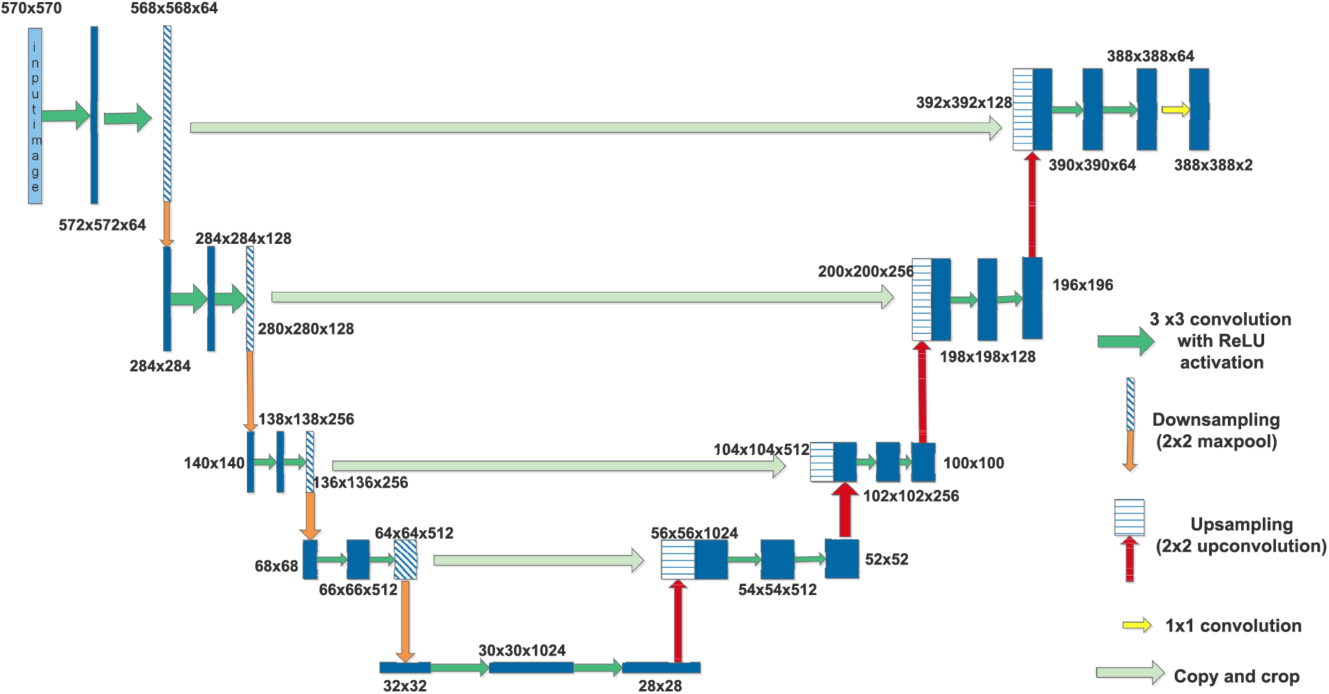
Figure 1: U-Net for image denoising

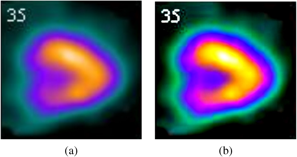
Figure 2: (a) Original image (b) Denoised image

4.1.2 Attenuation Correction with CNN

The image generated by the denoising model is subjected to attenuation correction. From a given set of denoised images X, an image x∈X, the attenuation correction method should make a mapping between the input image x and the attenuation corrected image y∈Y, i.e., ℱ≀: X⇢Y with proper parameters ≀∈Rn. In unsupervised learning, for N parameters to be defined to design the predictor ℱ≀ to minimize the error E as follows:

E=1N∑i=1Nℒ(ℱ≀(xi),yi)(4)

ℒ is the desired loss, and the learning process should find the best values among the pool of optimal values as following:

ℱ≀i(x)∈ℱ≀1(x), ℱ≀2(x),…ℱ≀M(x), M∈N(5)

The best predictor ℱ≀i(x) has the objective function of minimizing loss to find the best training parameters, as given in (6). In this case, the predicting CNN architecture learns in M different ways.

ℒ(ℱ≀(xi),yi)=minj∈[1,M]L(Foi(x),yi)(6)

The architecture of the CNN is shown in Fig. 3. A convolution network with twenty layers is used to perform the attenuation correction. Except for the last layer, all the remaining layers are fully connected softmax layers with 3 × 3 kernels followed by batch normalization and rectified linear units (ReLU), and to speed up the process, a shortcut connection between each pair of 3 × 3 filters is also used. In the dilated convolutions, for the middle seven layers, stride 2 is used, and for the last six layers, stride 4 is used. This structure can handle the receptive field’s exponential growth while keeping the input pictures’ original resolution. The output of attenuation correction is shown in Fig. 4.

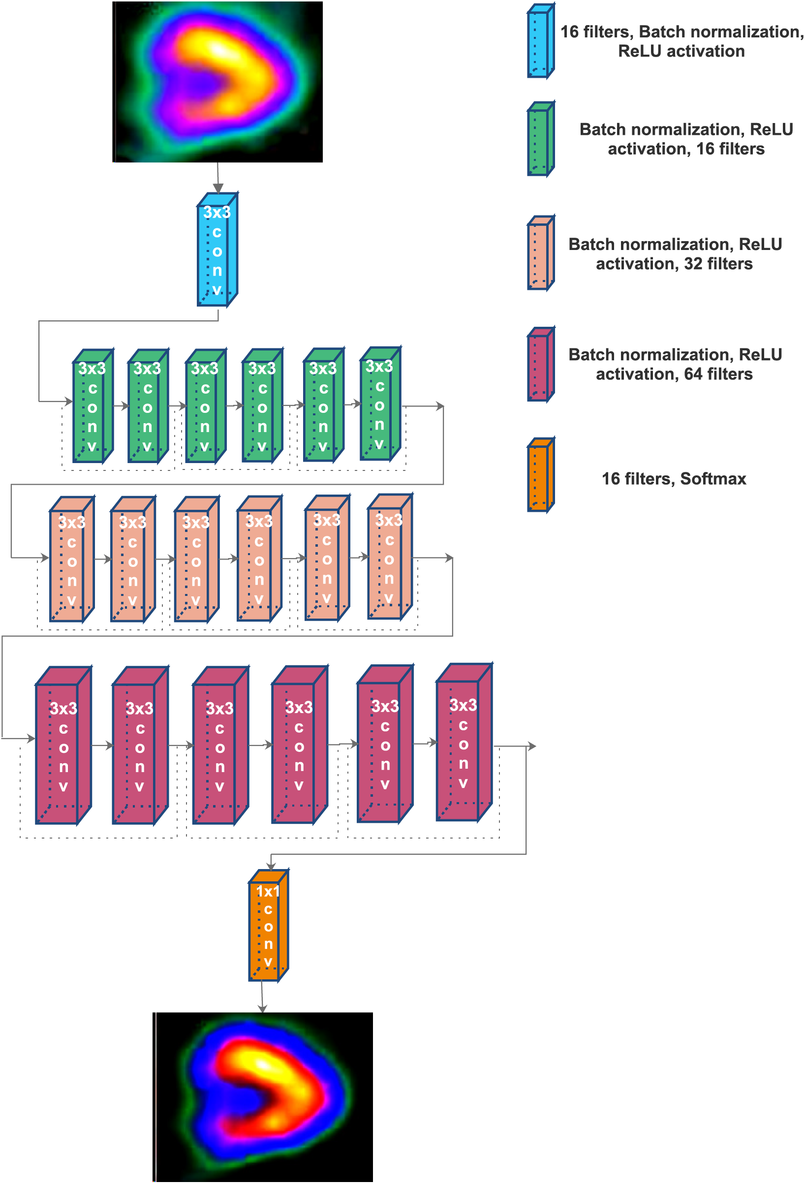
Figure 3: The architecture of residual network for attenuation correction

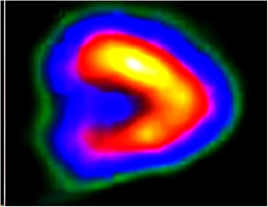
Figure 4: Output of attenuation correction

4.2 Classification

The classification process is classifying the given image as either normal or abnormal. The classification process has three phases: feature extraction, feature selection and classification. To perform this, an MSDC network is used. The objective function (S) of the classification function is expressed as

S:Z→CNor, CAbNor(7)

where, CNor represents normal pixel and CAbNor represents abnormal pixel. An MSDC network is used to extract the features and classify them. In deep learning models, the fully connected layers identify the patterns based on the extracted feature maps from the convolutional layers that produce the feature maps. Convolution layers are, therefore, essential to deep learning models. The locally connected patterns from the local receptive fields can be extracted using these layers to extract certain basic features like edges, corner points, oriented edges, etc. [46].

Additionally, it is invariant to the shift and distortion of the input image due to the utilization of local receptive fields. Each convolution layer has a collection of filters or kernels used to execute the convolution operation on the input picture. The formal definition of the convolution operation is as follows: Consider a discrete function F:Z2→R, Let ℘i=[−i,i]2∩Z2 and f:℘i→R is a filter with a size of (2i+1)2. The convolution operation expressed as

(F×f)(x)=∑y+z=xF(y)f(z)(8)

Although conventional convolution offers a method for capturing local patterns, it is frequently important to capture the broader context to increase the discriminative power of the feature maps. Yu et al. [47] offered the idea of dilated convolution. Dilated convolution’s main principle is introducing a few “gaps” (in this case, ∂) between pixels in convolution filters. Increasing the image resolution is the goal. Dilated convolution aids in exponentially expanding the network’s field of view so that more information about a larger environment can be obtained at a reduced cost. As a result, semantic segmentation frameworks frequently use it. In addition to resolving the vanishing gradient issue, dilated convolution speeds up network training. Assuming that ∂ is the dilation factor, then the convolution operator is redefined as

(Fxdf) (x)= ∑y+∂z=xF(y)f(z)(9)

As Lei et al. [48] demonstrated in their work, dilated convolution may not be very useful when utilized in a classification task. Primarily because the dilated convolution’s gaps, which have fixed dilation rates, could cause specific relevant pixels to be skipped, resulting in a loss of continuity information. Multi-scale dilated convolution is considered in the current scope of the work as a solution to this problem. In multi-scale dilated convolution, the gaps caused by higher-order dilation are filled in by lower-order dilations, eliminating the possibility of information loss and capturing a greater context at several scales. The formal definition of the multi-scale dilated convolution process employed here is estimated by

ðMSDC(X)=max∂{R(((Fx∂f)(x))}Where,R(x)={0(Fx∂f) (x)if (Fx∂f) (x) ≤ θotherwise(10)

Fig. 5 shows how the multiscalar diluted convolution works with ∂ values as 1, 2 and 3.

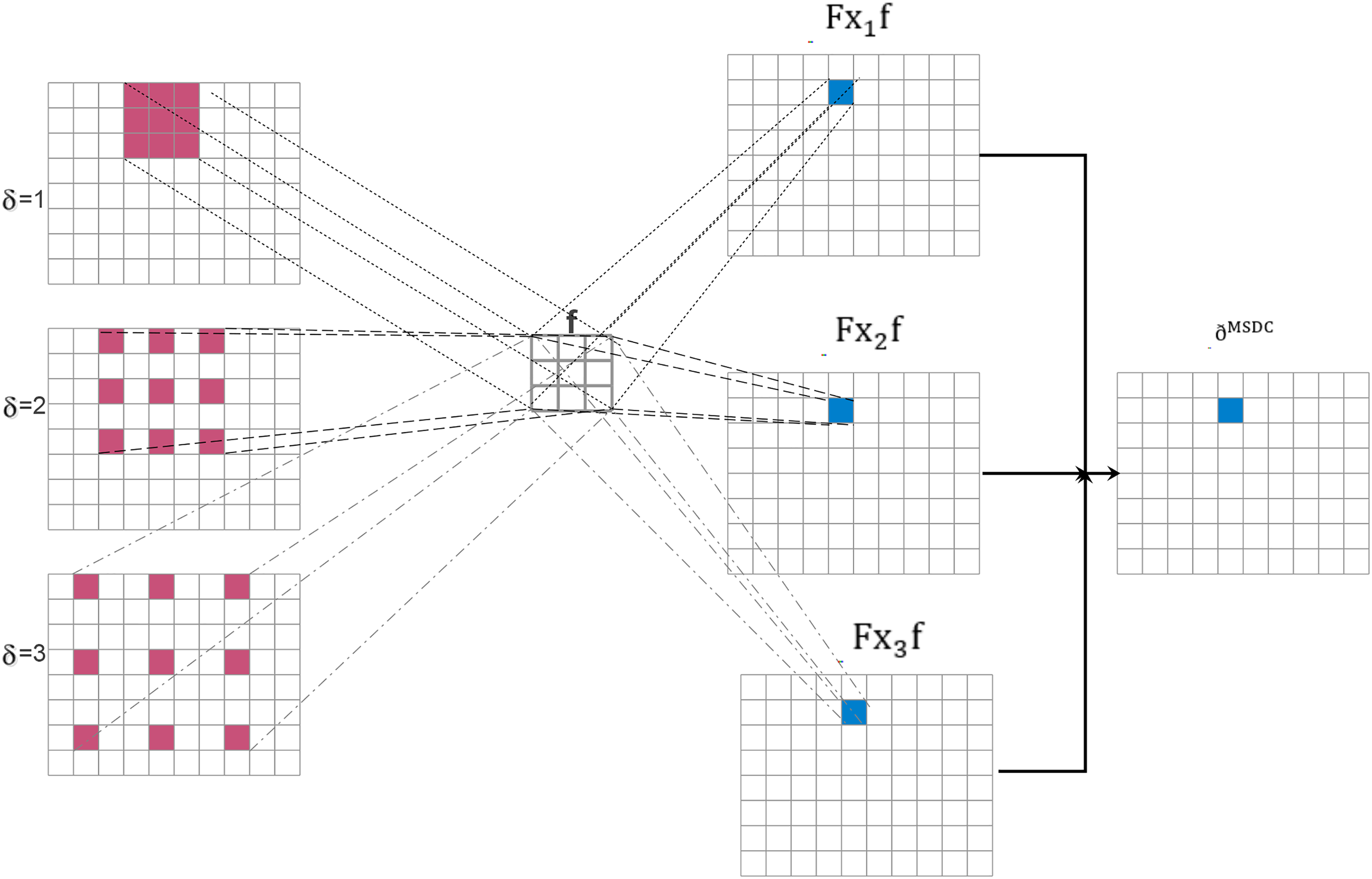
Figure 5: Multiscale diluted convolution with δ=1,2 and 3

A deep convolution neural network is used to perform MSDC. The model has three diluted convolution layers with 32 (stride 2), 64 (stride 4), and 128 (stride 1) filters, respectively. The size of all these filters is 3×3. The pooling layer comes after that. It is essential to record the relative position of the features retrieved from the input image rather than their exact location. Because the network may become sensitive to shift and distortion due to learning the precise placement of the features. By lowering the resolution of the feature maps, layer pooling or sub-sampling techniques decrease the likelihood of learning precise placements. As a result, after each MSDC layer in this study, a max pooling layer with a 2×2 kernel is utilized. The ReLU activation function is used in all these layers. Finally, a pair of fully connected layers with a dropout rate of 0.5 is also used. This helps in avoiding overfitting. Finally, a softmax layer is used to find the likelihood of each class.

In a convolutional neural network (CNN), the initial layer typically employs a relatively modest quantity of filters, often around 32. These filters are specifically designed to capture fundamental characteristics from the input photos. The network, equipped with 32 filters, can identify elementary patterns such as edges, textures, or fundamental shapes. Every filter analyzes the input image to generate feature maps that accentuate fundamental characteristics. These feature maps are subsequently employed in subsequent layers to construct increasingly intricate representations. When visualizing these 32 filters, one often observes a collection of abstract patterns with a concentration on essential visual features.

The selection of a dropout rate of 0.5 and the Adam optimizer for a CNN model is substantiated by both theoretical and empirical evidence. A dropout rate of 0.5 implements balanced regularization by randomly excluding 50% of neurons during training, hence preventing the model from becoming excessively reliant on particular neurons. This improves generalization, mitigates overfitting, and promotes the model’s robustness, particularly for intricate applications such as image recognition. Empirical evidence indicates that a 0.5 dropout rate is successful across many CNN designs. Conversely, the Adam optimizer is exceptionally efficient and extensively utilized because of its adaptive learning rate mechanism, which modifies the learning rate for each parameter according to the first and second moments of the gradients. This property, along with the advantages of both root mean square propagation (RMSProp) and momentum techniques, allows Adam to effectively manage noisy gradients and sparse data, facilitating rapid convergence without necessitating substantial hyperparameter optimization. Moreover, Adam’s efficacy and scalability render it appropriate for extensive datasets often associated with CNN models. The combination of a dropout rate of 0.5 and the Adam optimizer establishes a strong foundation for training CNNs, resulting in enhanced generalization and expedited convergence.

As the depth of the network develops, the number of filters often increases to enable the model to capture more complex information from the input images. The convolutional layer with 64 filters has a greater capacity to identify a broader spectrum of features and patterns in comparison to a layer with only 32 filters. The enhanced capacity allows the network to identify more intricate patterns, such as combinations of edges or textures, and to get a deeper knowledge of the finer details in the input data. When visualizing 64 filters, you may observe a greater variety and intricacy in patterns compared to filters in earlier layers, indicating an improved capability to extract intricate features.

When employing a substantial quantity of filters, such as 128, in the deeper layers of a CNN, the network becomes capable of extracting intricate and advanced characteristics from the input images. The network’s increased capacity, due to the utilization of 128 filters, allows for enhanced learning and representation of intricate patterns and higher-level abstractions. These filters can identify complex patterns, specific components of objects, and more conceptual characteristics, which enhances the depth and subtlety of the data analysis. When displaying 128 filters, a diverse range of intricate and elaborate patterns will be observed, showcasing the network’s capacity to analyze and comprehend a wide array of visual data. The increased number of filters improves the network’s ability to accurately identify and categorize a wider range of intricate and varied items in images. The convolution filters are shown in Fig. 6. The output of the three filters is shown in Fig. 7. These features are used to perform diluted convolution followed by a max pooling layer.

Figure 6: (a) 32 convolution filters (b) 64 convolution filters (c) 128 convolution filters

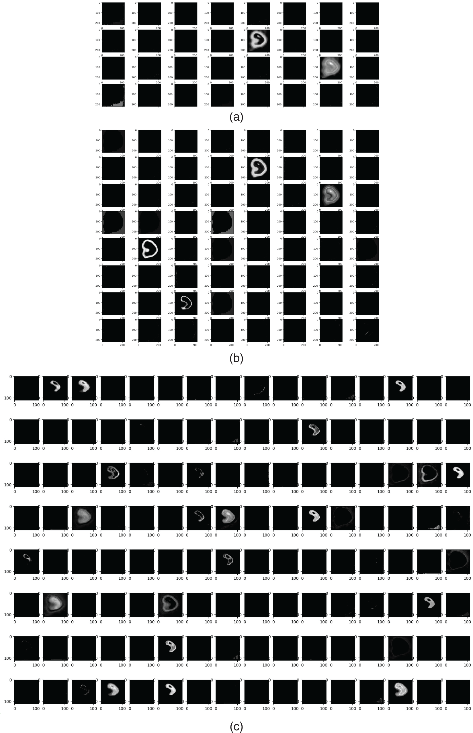
Figure 7: Features from (a) 32 filters, (b) 64 filters (c) 128 filters

5  Results and Discussion

The suggested methodology was evaluated utilizing the Anaconda runtime environment. It offers enhanced GPUs, more RAM, and expanded disk space, rendering it suitable for training large-scale parallel machine learning and deep learning models. We utilized Python 3.6 along with other Python libraries such as TensorFlow and Keras to implement the proposed models. The dataset was imported utilizing the OpenCV library, while the scikit-learn package was employed for its partitioning and result computation. Matplotlib was utilized to depict the plots. Furthermore, the subsequent specifications pertain to the computer’s key components: Intel Core i5 CPU at 2.40 GHz, NVIDIA Quadro RTX 3000, 32 GB of RAM, and more components. 64-bit operating system with x64 architecture. Dropout at a rate of 0.2 is employed in all three models to prevent overfitting. The Adam optimizer is utilized for hyperparameter optimization.

5.1 Analysis of Denoising

The proposed U-Net architecture is compared with the existing denoising neural network architectures like FDnCNN [49], NLCNN [50], UDNET [51], FC-AIDE [52], and FOCNet [53]. The output of all these methods is compared with the proposed U-Net architecture. Table 2 compares the proposed method with the state-of-the-art denoising models with a corresponding peak signal-to-noise ratio (PSNR). The average PSNR value was calculated for all samples in the test set. FDnCNN model registers an average PSNR of 30.7, NLCNN registers 26, UDNET registers 38.2, FC-AIDE registers 37.4, FOCNet registers 39.2 and the proposed U-Net model achieves the maximum of its case of average PSNR with 39.7. The visual output, as well as the quantitative value of PSNR, shows that the proposed U-Net denoising outperforms other methods.

5.2 Analysis of Attenuation Correction

The attenuation correction methods like 3D U-Net, generative adversarial network (GAN), and ProGAN models from the same GitHub repository [54] are compared with the proposed ResNET model. Table 3 summarizes the output obtained from the attenuation correction methods, and the visual outputs show that the proposed ResNET outperforms the other CNN models.

5.3 Comparison of Classification

The proposed MDSC-Net is compared with five deep convolution neural network models. The details of the layers of the architectures are given in Table 4. Among the five architectures, AlexNet is the standard convolution neural network model. Others are a simple convolution neural network, a CNN with an attention module, a CNN with a residual module, and a CNN with an attention and residual module [55].

The basic CNN model serves as a fundamental architecture for classification jobs. It is engineered to incrementally extract characteristics from the input image by the use of convolutional filters that capture spatial hierarchies within the data. The model initiates with a (64×(11×11)) convolutional layer, employing a stride of 4 and padding of 2, which identifies fundamental features like edges and textures. This is succeeded by a max-pooling layer that diminishes the spatial dimensions and aids in preserving significant features while reducing computational complexity. Supplementary convolutional layers utilizing (128×(7×7)), (128×(5×5)), and (256×(3×3)) filters enhance the feature extraction process, identifying increasingly intricate patterns as the network deepens. Following multiple layers of convolutions and max-pooling, two fully connected layers, each including 1024 neurons, consolidate the recovered features for classification purposes. A concluding softmax layer generates probability for the two classes within the dataset. This model demonstrates proficiency in learning spatial hierarchies and is frequently employed as a benchmark for picture classification tasks.

The CNN with an attention module enhances the conventional CNN by including a channel attention mechanism. The model’s importance resides in its capacity to prioritize the most critical feature maps, enabling it to discern which features are most pertinent to the classification task. The design commences akin to the conventional CNN with a (64×(11×11)) convolutional layer, succeeded by max-pooling. A channel attention module is subsequently employed, which dynamically modifies the significance of each feature map prior to transmitting the information to deeper layers. The following layers, comprising (128×(7×7)), (128×(5×5)), and (256×(3×3)) convolutional layers, are intended to extract mid- and high-level features. An additional attention module is incorporated in the later phases to enhance the network’s concentration. The network is concluded with fully connected layers and a softmax output. This attention-augmented CNN boosts feature differentiation and elevates performance on jobs where certain features are paramount for categorization.

The CNN incorporating a residual module mitigates the issue of vanishing gradients, which complicates the training of deep networks. Residual modules, used in the ResNet design, enable the model to acquire identity mappings by bypassing one or more layers. This facilitates improved gradient flow during backpropagation, permitting the network to achieve greater depth without encountering the degradation issue. The design initiates with a (64×(11×11)) convolutional layer, succeeded by max-pooling. A residual module is implemented subsequent to the initial layers, incorporating skip connections that facilitate the preservation of information flow. Subsequent convolutional layers use (128×(7×7)), (128×(5×5)), and (256×(3×3)) filters, each enhancing the feature maps. A supplementary residual module is implemented in the subsequent layers, enhancing the network’s robustness and facilitating training. The model concludes with two fully connected layers and a softmax output layer. The remaining connections render this model exceptionally efficient for jobs necessitating deep architectures.

This model integrates the advantages of both attention and residual modules, offering a robust framework for categorization tasks. The design commences with a (64×(11×11)) convolutional layer, succeeded by max-pooling. A channel attention module is implemented early in the network, enabling the model to concentrate on the most pertinent feature maps. A residual module is incorporated to facilitate seamless gradient flow and permit deeper network training. The following convolutional layers, including (128×(7×7)), (128×(5×5)), and (256×(3×3)), systematically extract increasingly intricate features. A secondary channel attention module and an additional residual module are incorporated later in the network to augment the feature extraction process further. The model terminates with fully connected layers and a softmax output layer. This hybrid methodology, integrating attention and residual modules, improves feature selection and facilitates the training of deeper networks, rendering it exceptionally successful for intricate classification problems.

AlexNet is a historically noteworthy convolutional neural network, as it was among the first to showcase the efficacy of deep learning in picture categorization, particularly during the ImageNet competition in 2012. The architecture has multiple convolutional and max-pooling layers intended to extract characteristics from input photos systematically. The initial convolutional layer employs (64×(11×11)) filters with a stride of 4, therefore diminishing the image dimensions while extracting fundamental characteristics such as edges. Max-pooling layers are strategically placed inside the network to diminish spatial dimensions while preserving only the most significant information. The deeper convolutional layers, utilizing (256×(3×3)) and (384×(3×3)) filters, capture more intricate and abstract patterns. Two fully connected layers of 1024 neurons amalgamate the feature maps, while a softmax layer delivers the ultimate classification into two categories. The success of AlexNet solidified CNNs as a preeminent method in computer vision applications.

The confusion matrix of the five state-of-the-art architectures and the proposed architecture is shown in Fig. 8. From these confusion matrices, all the CNN models are working well on finding the normal and abnormal pixels in the SPECT image. The proposed MSDC-Net outperforms the other methods by correctly classifying 23 normal images out of 24 and 22 abnormal images out of 24 in the test set.

Accuracy=TP+TNTP+TN+FP+FN(11)

Precision=TPTP+FP(12)

Sensitivity=TPTP+FN(13)

Specificity=TNTN+FP(14)

F1-score=2×Precision ×SensitivityPrecision+Sensitivity(15)

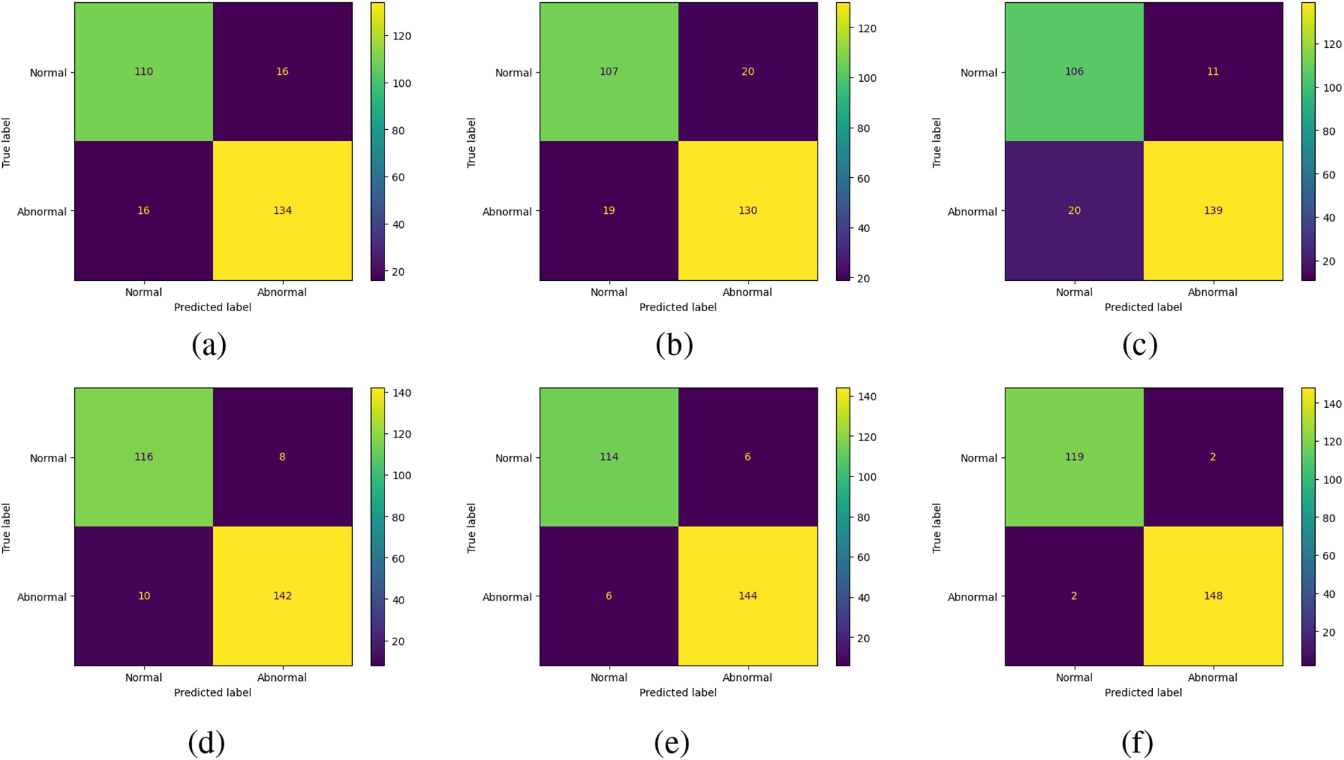
Figure 8: Confusion matrix for (a) CNN, (b) CNN with attention module, (c) CNN with the residual module, (d) CNN with attention and residual module, (e) AlexNet, and (f) Proposed MSDC-Net

Along with the true positive, true negative, false positive, and false negative, the other classification metrics, accuracy, precision, sensitivity/recall, specificity, and F1-scores, are analyzed as given in (11) to (15). These metrics are shown in Fig. 9.

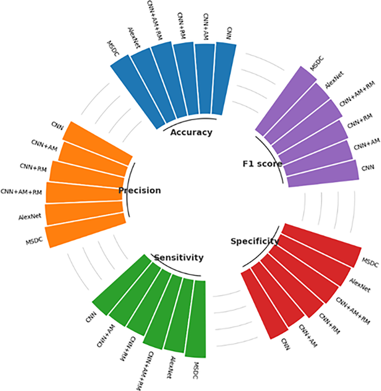
Figure 9: Comparison of classification metrics

The proposed MSDC-Net model achieves a remarkable accuracy of 0.96739, signifying its ability to accurately forecast approximately 97% of the cases. The CNN+AM model has the lowest accuracy, with a precision of 0.8587, indicating that it has a higher number of errors compared to the other models. The AlexNet and CNN+AM+RM models exhibit a commendable accuracy of 0.93478, positioning them as strong competitors to the Proposed MSDC Net. The Proposed MSDC Net model once again demonstrates a precision of 0.98347, signifying that about 98% of its positive predictions are accurate. AlexNet exhibits excellent performance, with an accuracy of 0.95.

The CNN model, with a precision of 0.87302, exhibits the lowest capacity to reliably forecast positive cases in comparison to the other models. The proposed MSDC-Net model obtains a sensitivity of 0.94444, indicating that it correctly recognizes approximately 94% of all positive cases. The CNN+RM model exhibits a sensitivity of 0.84127, which is the least favorable compared to the other models. This suggests that it is more likely to overlook positive situations in comparison. CNN+AM+RM and AlexNet both demonstrate a notable degree of sensitivity, rendering them proficient in detecting positive instances. The proposed MSDC-Net model exhibits a remarkable specificity of 0.98667, indicating its high efficiency in accurately identifying negative cases. The CNN+RM model exhibits a high level of specificity at 0.92667, while it is somewhat less proficient than the proposed MSDC-Net in accurately predicting negative outcomes. The specificity of CNN+AM is 0.86667, indicating a lower ability to accurately identify genuine negatives.

The proposed MSDC-Net achieves an F1-score of 0.96356, which demonstrates its remarkable ability to maintain a balance between precision and recall. The CNN model exhibits the lowest F1-score of 0.87302, indicating inferior performance in achieving a balance between precision and recall when compared to the other models. The F1-scores of CNN+AM+RM and AlexNet are 0.928 and 0.92683, respectively, indicating their effectiveness in achieving a balanced trade-off between precision and recall. The Proposed MSDC Net demonstrates superior performance compared to other models in all measures, exhibiting the greatest values in accuracy, precision, sensitivity, specificity, and F1-score. This indicates that it is the most dependable model for the CAD detection task.

High true positive rates (TPR = Sensitivity) and low false positive rates (FPR = 1-Specificity) are desired characteristics for a classifier. The area under the ROC curve, or AUC value, is the ratio of true positive rates (y-axis) to false positive rates (x-axis). The probability that a randomly selected positive image will be ranked higher than a randomly selected negative image is the statistical explanation for the AUC value. As a result, the classifier performs better the closer the AUC value is to 1. The AUC for normal images is shown in Fig. 10. The result shows that the proposed MSDC-Net has an AUC value of 0.98, CNN has 0.78, CNN with attention module and AlexNet has 0.79, and CNN with the residual model has a value of 0.85. Thus, MSDC-Net has an AUC value closer to 1.

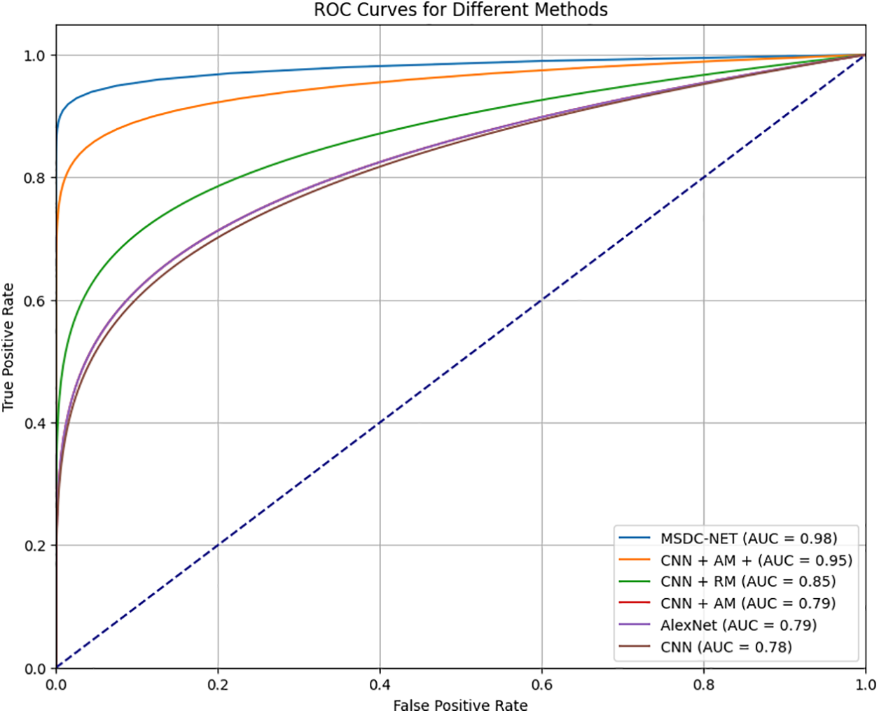
Figure 10: Comparison of AUC

The proposed MSDC-Net model is trained for 300 epochs with a learning rate of 0.001. The training and validation accuracy and loss without preprocessing is shown in Fig. 11a and the training and validation accuracy and loss with preprocessing is shown in Fig. 11b across 300 epochs. Magboo et al. [56] used the same dataset for CAD detection using well-known CNN models like VGG16, DenseNet121, InceptionV3 and ResNet50. These models were trained for 300 epochs and compared to the proposed MSDC-Net. The comparison was done with and without preprocessing in terms of accuracy, recall, precision and F1-score. Table 5 summarizes the obtained results. The results show that the proposed method registers the best classification performance with 93.75% and 95.83% of accuracy without and with preprocessing, respectively.

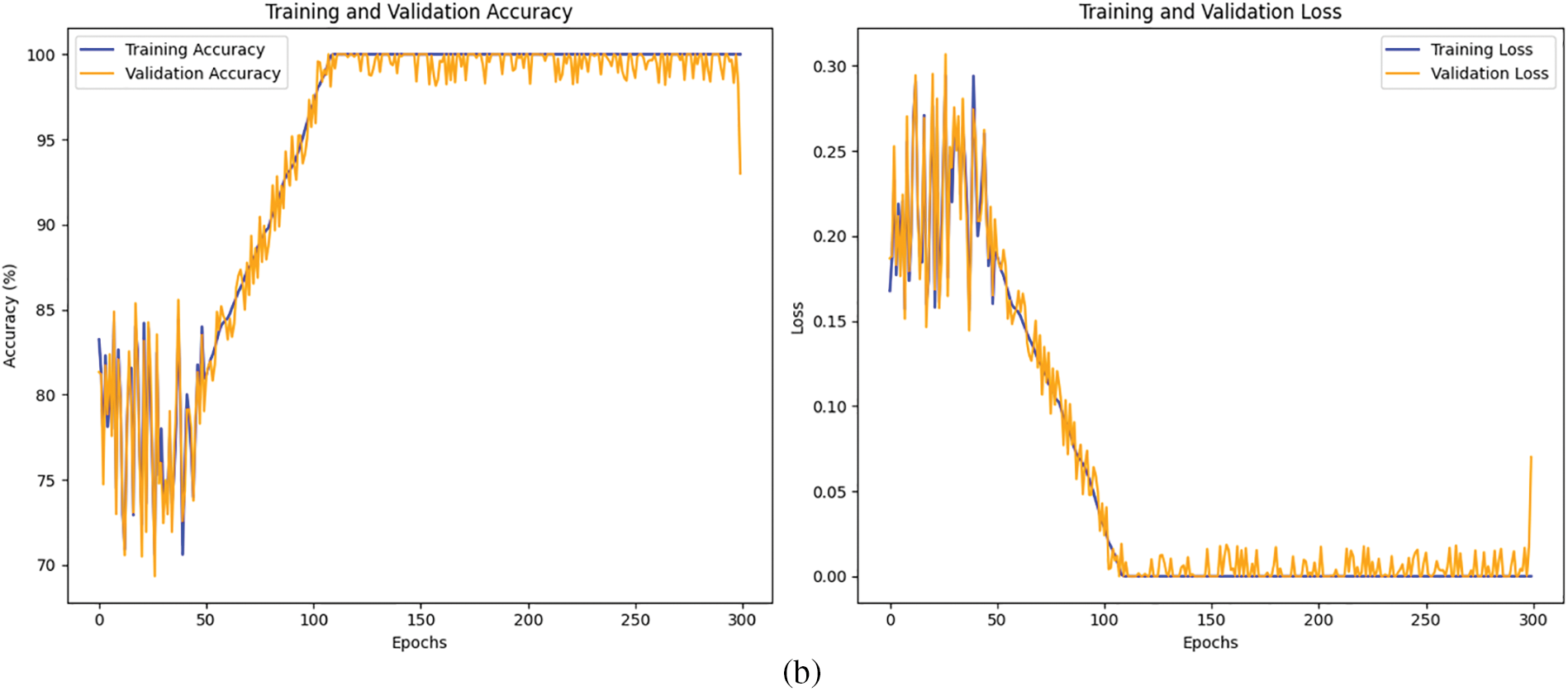
Figure 11: (a) Training and validation accuracy and loss without preprocessing (b) Training and validation accuracy and loss with preprocessing

6  Conclusion

Deep learning has shown that it can work independently and assist in the healthcare industry. In more detail, CNNs gain from their capacity to receive images as input and achieve high image classification accuracy. The proposed framework has a three-step classification method with two preprocessing, denoising, and attenuation correction. These two processes enhance the original image and make the image more precise for an efficient classification process. The MSDC-based classification method learns features more efficiently by using feature extraction on different scales. The classification performance is compared with the state-of-the-art models. The proposed method ensures high accuracy with 96%. The proposed method is a binary classification model to detect the CAD using SPECT-MPI. Its time complexity is high as it contains three deep learning models. The proposed method can process the image data only, which does not consider the clinical and biological data. To address these limitations, in the future, the adaptation of lightweight design and appropriate optimization can be included in all three architectures to improve the time complexity of the entire framework. The sub-classes like Infarction and Ischemia will be diagnosed with a multi-class classification framework. The proposed method can be extended to a multi-modal model to process diagnosis images and biological and clinical data.

Acknowledgement: We would like to thank our institutions for permitting us to carry out this research. We acknowledge the patients who participated in the data collection process of the datasets used.

Funding Statement: The present research has been conducted by the Research Grant of Kwangwoon University in 2024.

Author Contributions: Conceptualization, A. Robert Singh; Data curation, A. Robert Singh and Suganya Athisayamani; Formal analysis, A. Robert Singh; Funding acquisition, Bhanu Shrestha; Methodology, A. Robert Singh and Suganya Athisayamani; Project administration, Bhanu Shrestha and Gyanendra Prasad Joshi; Resources, Bhanu Shrestha and Gyanendra Prasad Joshi; Software, Suganya Athisayamani; Supervision, Bhanu Shrestha and Gyanendra Prasad Joshi; Validation, Bhanu Shrestha and Gyanendra Prasad Joshi; Visualization, Suganya Athisayamani and Bhanu Shrestha; Writing—original draft, A. Robert Singh; Writing, review & editing, Gyanendra Prasad Joshi. All authors reviewed the results and approved the final version of the manuscript.

Availability of Data and Materials: The SPECT MPI dataset. Available online: https://www.kaggle.com/datasets/selcankaplan/spect-mpi (accessed on 05 November 2024).

Ethics Approval: Not applicable.

Conflicts of Interest: The authors declare no conflicts of interest to report regarding the present study.

References

1. Chen JJ, Su TY, Chen WS, Chang YH, Lu HHS. Convolutional neural network in the evaluation of myocardial ischemia from CZT SPECT myocardial perfusion imaging: comparison to automated quantification. Appl Sci. 2021;11(2):514. doi:10.3390/app11020514. [Google Scholar] [CrossRef]

2. Cassar A, Holmes DR, Rihal CS, Gersh BJ. Chronic coronary artery disease. Diagn Manag. 2009 Dec;84(12):1130–46. doi:10.4065/mcp.2009.0391. [Google Scholar] [PubMed] [CrossRef]

3. Bruyant PP. Analytic and iterative reconstruction algorithms in SPECT. J Nucl Med. 2002 Oct;43(10):1130–46. [Google Scholar]

4. Tsui BMW. The AAPM/RSNA physics tutorial for residents. Physics of SPECT. RadioGraphics. 1996 Jan;16(1):173–83. doi:10.1148/radiographics.16.1.173. [Google Scholar] [PubMed] [CrossRef]

5. Van Laere K, Koole M, Lemahieu I, Dierckx R. Image filtering in single-photon emission computed tomography: principles and applications. Comput Med Imaging Graph. 2001 Mar;25(2):127–33. doi:10.1016/s0895-6111(00)00063-x. [Google Scholar] [PubMed] [CrossRef]

6. Slart RHJA, Williams MC, Juarez-Orozco LE, Rischpler C, Dweck MR, Glaudemans AWJM, et al. Position paper of the EACVI and EANM on artificial intelligence applications in multimodality cardiovascular imaging using SPECT/CT, PET/CT, and cardiac CT. Eur J Nucl Med Mol Imaging. 2021 Apr;48(5):1399–413. doi:10.1007/s00259-021-05341-z. [Google Scholar] [PubMed] [CrossRef]

7. Garcia EV. SPECT attenuation correction: an essential tool to realize nuclear cardiologyâs manifest destiny. J Nucl. Cardiol. 2007 Jan;14(1):16–24. doi:10.1016/j.nuclcard.2006.12.144. [Google Scholar] [PubMed] [CrossRef]

8. Zhang YC, Kagen A. Machine learning interface for medical image analysis. J Digit Imaging. 2017 Oct;30(5):615–21. doi:10.1007/s10278-016-9910-0. [Google Scholar] [PubMed] [CrossRef]

9. Arsanjani R, Xu Y, Dey D, Vahistha V, Shalev A, Nakanishi R, et al. Improved accuracy of myocardial perfusion SPECT for detection of coronary artery disease by machine learning in a large population. J Nucl. Cardiol. 2013 May;20(4):553–62. doi:10.1007/s12350-013-9706-2. [Google Scholar] [PubMed] [CrossRef]

10. Papandrianos N, Papageorgiou E. Automatic diagnosis of coronary artery disease in SPECT myocardial perfusion imaging employing deep learning. Appl Sci. 2021 Jul;11(14):6362. doi:10.3390/app11146362. [Google Scholar] [CrossRef]

11. Savvopoulos C, Spyridonidis T, Papandrianos N, Vassilakos P, Alexopoulos D, Apostolopoulos DJ. CT-based attenuation correction in Tl-201 myocardial perfusion scintigraphy is less effective than non-corrected SPECT for risk stratification. J Nucl Cardiol. 2014 Feb;21(3):519–31. doi:10.1007/s12350-014-9867-7. [Google Scholar] [PubMed] [CrossRef]

12. Juan A, Yang Y, Pretorius PH, Johnson KL, King MA, Wernick MN. Improving diagnostic accuracy in low-dose SPECT myocardial perfusion imaging with convolutional denoising networks. IEEE Transac Med Imaging. 2020 Mar;39(9):2893–903. doi:10.1109/TMI.2020.2979940. [Google Scholar] [PubMed] [CrossRef]

13. Willett R, Nowak R. Platelets: a multiscale approach for recovering edges and surfaces in photon-limited medical imaging. IEEE Trans Med Imaging. 2003 May;22(3):332–50. doi:10.1109/tmi.2003.809622. [Google Scholar] [PubMed] [CrossRef]

14. Johnson LC, Shokouhi S, Peterson TE. Reducing multiplexing artifacts in multi-pinhole SPECT with a stacked silicon-germanium system: a simulation study. IEEE Trans Med Imaging. 2014 Jul;33(12):2342–51. doi:10.1109/tmi.2014.2340251. [Google Scholar] [PubMed] [CrossRef]

15. Van Audenhaege K, Vanhove C, Vandenberghe S, Van Holen R. The evaluation of data completeness and image quality in multiplexing multi-pinhole SPECT. IEEE Trans Med Imaging. 2015 Feb;34(2):474–86. doi:10.1109/tmi.2014.2361051. [Google Scholar] [PubMed] [CrossRef]

16. Hachamovitch R, Berman DS, Shaw LJ, Kiat H, Kiat H, Cohen I, et al. Incremental prognostic value of myocardial perfusion single photon emission computed tomography for the prediction of cardiac death differential stratification for risk of cardiac death and myocardial infarction. Circulation. 1998 Feb;97(6):535–43. doi:10.1161/01.cir.97.6.535. [Google Scholar] [PubMed] [CrossRef]

17. Arabi H, Kamali Asl AR. Feasibility study of a new approach for reducing of partial volume averaging artifact in CT scanner. In: IEEE 2010 17th Iran Conf Biomed Eng (ICBME2010; p. 1–4. doi:10.1109/icbme.2010.5704968. [Google Scholar] [CrossRef]

18. Cuocolo A. Attenuation correction for myocardial perfusion SPECT imaging: still a controversial issue. Eur J Nucl Med Mol Imaging. 2011 Aug;38(10):1887–9. doi:10.1007/s00259-011-1898-6. [Google Scholar] [PubMed] [CrossRef]

19. Sajedi S, Zeraatkar N, Moji V, Farahani MH, Sarkar S, Arabi H, et al. Design and development of a high resolution animal SPECT scanner dedicated for rat and mouse imaging. Nucl Instrum Meth A. 2014 Mar;741:169–76. doi:10.1016/j.nima.2014.01.001. [Google Scholar] [CrossRef]

20. Fukushima Y, Kumita S. Cardiac SPECT/CT imaging: CT attenuation correction and SPECT/CT hybrid imaging. Int J Radiol Med Imaging. 2016 Jul;2016(2):113. doi:10.15344/2456-446x/2016/113. [Google Scholar] [CrossRef]

21. Raza H, Jadoon LK, Mushtaq S, Jabeen A, Maqbool M, Ain MU, et al. Comparison of non-attenuation corrected and attenuation corrected myocardial perfusion SPECT. Egypt J Radiol Nucl Med. 2016 Sep;47(3):783–92. doi:10.1016/j.ejrnm.2016.05.006. [Google Scholar] [CrossRef]

22. Mostafapour S, Arabi H, Gholamiankhah F, Razavi-Ratki SK, Parach AA. Tc-99m (methylene diphosphonate) SPECT quantitative imaging: impact of attenuation map generation from SPECT-non-attenuation corrected and MR images on the diagnosis of bone metastasis. Int J Radiat Res. 2021 Apr;19(2):299–308. doi:10.52547/ijrr.19.2.7. [Google Scholar] [CrossRef]

23. Genovesi D, Giorgetti A, Gimelli A, Kusch A, DâAragona Tagliavia I, Casagranda M, et al. Impact of attenuation correction and gated acquisition in SPECT myocardial perfusion imaging: results of the multicentre SPAG (SPECT Attenuation Correction vs Gated) study. Eur J Nucl Med Mol Imaging. 2011 Jun;38(10):1890–8. doi:10.1007/s00259-011-1855-4. [Google Scholar] [PubMed] [CrossRef]

24. Singh B, Bateman TM, Case JA, Heller GV. Attenuation artifact, attenuation correction, and the future of myocardial perfusion SPECT. J Nucl Cardiol. 2007 Apr;14(2):153–64. doi:10.1016/j.nuclcard.2007.01.037. [Google Scholar] [PubMed] [CrossRef]

25. Esteves F, Santana CA, Folks RD, Faber TL, Bateman TM, Garcia EV. 37.03 Attenuation-corrected adenosine stress Tc-99m estamibi myocardial perfusion SPECT normal files: prospective validation and comparison to exercise stress normal files. J Nucl Cardiol. 2005 Jul;12(4):S124–5. doi:10.1016/j.nuclcard.2005.06.080. [Google Scholar] [CrossRef]

26. Masood Y, Liu YH, DePuey G, Taillefer R, Araujo LI, Allen S, et al. Clinical validation of SPECT attenuation correction using X-ray computed tomographyâderived attenuation maps: multicenter clinical trial with angiographic correlation. J Nucl Cardiol. 2005 Nov;12(6):676–86. doi:10.1016/j.nuclcard.2005.08.006. [Google Scholar] [PubMed] [CrossRef]

27. Zaidi H, Hasegawa B. Determination of the attenuation map in emission tomography. J Nucl Cardiol. 2003 Feb;44(2):291–315. [Google Scholar]

28. Goetze S, Brown TLY, Lavely WC, Zhang Z, Bengel FM. Attenuation correction in myocardial perfusion SPECT/CT: effects of misregistration and value of reregistration. J Nucl Cardiol. 2007 Jul;44(2):291–315. [Google Scholar]

29. Saleki L, Ghafarian P, Bitarafan-Rajabi A, Yaghoobi N, Fallahi B, Ay MR. The influence of misregistration between CT and SPECT images on the accuracy of CT-based attenuation correction of cardiac SPECT/CT imaging: phantom and clinical studies. Iran J Nucl Med. 2019 Jul;27(2):63–72. [Google Scholar]

30. Shi L, Onofrey JA, Liu H, Liu YH, Liu YH, Liu C. Deep learning-based attenuation map generation for myocardial perfusion SPECT. Eur J Nucl Med Mol Imaging. 2020 Mar;47(10):2383–95. doi:10.1007/s00259-020-04746-6. [Google Scholar] [PubMed] [CrossRef]

31. Marshall H, Stodilka RZ, Théberge J, Sabondjian E, Legros A, Deans L, et al. A comparison of MR-based attenuation correction in PET versus SPECT. Phys Med Biol. 2011 Jul;56(14):4613. doi:10.1088/0031-9155/56/14/024. [Google Scholar] [PubMed] [CrossRef]

32. Mehranian A, Arabi H, Zaidi H. Quantitative analysis of MRI-guided attenuation correction techniques in time-of-flight brain PET/MRI. NeuroImage. 2016;130:123–33. doi:10.1016/j.neuroimage.2016.01.060. [Google Scholar] [PubMed] [CrossRef]

33. Arabi H, Zaidi H. Truncation compensation and metallic dental implant artefact reduction in PET/MRI attenuation correction using deep learning-based object completion. Phy Med Bio. 2020 Sep;65(19):195002. doi:10.1088/1361-6560/abb02c. [Google Scholar] [PubMed] [CrossRef]

34. Arabi H, Bortolin K, Ginovart N, Garibotto V, Zaidi H. Deep learning-guided joint attenuation and scatter correction in multitracer neuroimaging studies. Hum Brain Mapp. 2020 May;41(13):3667–79. doi:10.1002/hbm.25039. [Google Scholar] [PubMed] [CrossRef]

35. Arabi H, Zaidi H. Deep learning-based metal artefact reduction in PET/CT imaging. Eur Radiol. 2021 Feb;31(8):6384–96. doi:10.1007/s00330-021-07709-z. [Google Scholar] [PubMed] [CrossRef]

36. Tankyevych O, Tixier F, Antonorsi N, Razzouki AF, Mondon R, Pinto-Leite T, et al. Can alternative PET reconstruction schemes improve the prognostic value of radiomic features in non-small cell lung cancer? Methods. 2021 Apr;188:73–83. doi:10.1016/j.ymeth.2020.11.002. [Google Scholar] [PubMed] [CrossRef]

37. Arabi H, Zeng G, Zheng G, Zheng G, Zaidi H. Novel adversarial semantic structure deep learning for MRI-guided attenuation correction in brain PET/MRI. Eur J Nucl Med Mol Imaging. 2019 Jul;46(13):2746–59. [Google Scholar] [PubMed]

38. Kaplan Berkaya S, Ak Sivrikoz I, Gunal S. Classification models for SPECT myocardial perfusion imaging. Comput Biol Med. 2020;123:103893. doi:10.1016/j.compbiomed.2020.103893. [Google Scholar] [PubMed] [CrossRef]

39. Papandrianos N, Feleki A, Papageorgiou E. Exploring classification of SPECT MPI images applying convolutional neural networks. In: Proceedings of the 25th Pan-Hellenic Conference on Informatics, PCI ’21, 2022; New York, NY, USA: Association for Computing Machinery; p. 483–9. doi:10.1145/3503823.3503911. [Google Scholar] [CrossRef]

40. Betancur J, Hu LH, Commandeur F, Sharir T, Einstein AJ, Fish MB, et al. Deep learning analysis of upright-supine high-efficiency SPECT myocardial perfusion imaging for prediction of obstructive coronary artery disease: a multicenter study. J Nucl Med. 2019 May;60(5):664–70. doi:10.2967/jnumed.118.213538. [Google Scholar] [PubMed] [CrossRef]

41. Betancur J, Commandeur F, Motlagh M, Sharir T, Einstein AJ, Bokhari S, et al. Deep learning for prediction of obstructive disease from fast myocardial perfusion SPECT: a multicenter study. JACC: Cardiovasc Imaging. 2018 Nov;11(11):1654–63. doi:10.1016/j.jcmg.2018.01.020. [Google Scholar] [PubMed] [CrossRef]

42. Liu H, Wu J, Wu J, Miller EJ, Liu C, Liu Y, et al. Diagnostic accuracy of stress-only myocardial perfusion SPECT improved by deep learning. Eur J Nucl Med Mol Imaging. 2021 Jan;48(9):2793–800. doi:10.1007/s00259-021-05202-9. [Google Scholar] [PubMed] [CrossRef]

43. Zahiri N, Asgari R, Razavi-Ratki SK, parach AA. Deep learning analysis of polar maps from SPECT myocardial perfusion imaging for prediction of coronary artery disease. Res Squ. 2021. doi:10.21203/rs.3.rs-1153347/v1. [Google Scholar] [CrossRef]

44. selcan kaplan. SPECT MPI. 2024. Available from: https://www.kaggle.com/datasets/selcankaplan/spect-mpi. [Accessed 2024]. [Google Scholar]

45. Anu P, Ramani G, Hariharasitaraman S, Robert Singh A, Athisayamani S. MRI denoising with residual connections and two-way scaling using unsupervised swin convolutional U-Net transformer (USCUNT). In: Thampi SM, Hu J, Das AK, Mathew J, Tripathi S, editors. Applied soft computing and communication networks. Singapore: Springer Nature Singapore; 2024. p. 419–33. doi:10.1007/978-981-97-2004-0_30. [Google Scholar] [CrossRef]

46. Iskander S, Iskandrian AE. Risk assessment using single-photon emission computed tomographic technetium-99m sestamibi imaging. J Am Coll Cardiol. 1998 Jul;32(1):57–62. doi:10.1016/s0735-1097(98)00177-6. [Google Scholar] [PubMed] [CrossRef]

47. Yu F, Koltun V. Multi-scale context aggregation by dilated convolutions. In: International Conference on Learning Representations, 2016; Caribe Hilton, San Juan, Puerto Rico, USA. [Google Scholar]

48. Lei X, Pan H, Huang X. A dilated CNN model for image classification. IEEE Access. 2019;7:124087–95. doi:10.1109/Access.6287639. [Google Scholar] [CrossRef]

49. Zhang K, Zuo W, Chen Y, Meng D, Zhang L. Beyond a gaussian denoiser: residual learning of deep CNN for image denoising. IEEE Transact Image Process. 2017;26(7):3142–55. doi:10.1109/TIP.83. [Google Scholar] [CrossRef]

50. Lefkimmiatis S. Non-local color image denoising with convolutional neural networks. In: 2017 IEEE Conference on Computer Vision and Pattern Recognition (CVPR), 2017; Honolulu, HI, USA; p. 5882–91. doi:10.1109/cvpr.2017.623. [Google Scholar] [CrossRef]

51. Lefkimmiatis S. Universal denoising networks: a novel CNN architecture for image denoising. In: 2018 IEEE/CVF Conference on Computer Vision and Pattern Recognition (CVPR), 2018; Salt Lake City, UT, USA; p. 3204–13. doi:10.1109/cvpr.2018.00338. [Google Scholar] [CrossRef]

52. Cha S, Moon T. Fully convolutional pixel adaptive image denoiser. In: 2019 IEEE/CVF International Conference on Computer Vision (ICCV), 2019; Seoul, Republic of Korea, p. 4159–68. doi:10.1109/iccv.2019.00426. [Google Scholar] [CrossRef]

53. Jia X, Liu S, Feng X, Zhang L. FOCNet: a fractional optimal control network for image denoising. In: 2019 IEEE/CVF Conference on Computer Vision and Pattern Recognition (CVPR), 2019; Long Beach, CA, USA; p. 6047–56. doi:10.1109/cvpr.2019.00621. [Google Scholar] [CrossRef]

54. C RR. DeepAttCorrection. 2024. Available from: https://github.com/RawthiL/PET_DeepAttCorrection. [Accessed 2024]. [Google Scholar]

55. Athisayamani S. CNN-models-SPECT. 2024. Available from: https://github.com/suganya-athisayamani/CNN-models-SPECT. [Accessed 2024]. [Google Scholar]

56. Magboo VPC, Magboo MSA. Diagnosis of coronary artery disease from myocardial perfusion imaging using convolutional neural networks. Procedia Comput Sci. 2023;218:810–7. doi:10.1016/j.procs.2023.01.061. [Google Scholar] [CrossRef]