Impact of Pollutant Concentration and Particle Deposition on the Radiative Flow of Casson-Micropolar Fluid between Parallel Plates

Nomenclature

1  Introduction

A fluid that exhibits microscopic phenomena like spin inertia and micro-rotational motions is called a micropolar fluid. Micropolar liquid is a type of non-Newtonian liquid. Initially, Eringen developed the concept of micropolar fluid. Micropolar fluids have applications in numerous industrial and biological processes, including the synthesis of polymers, the drawing of wire, the manufacturing of glass fiber, and the cooling process of metallic sheets. Ismael et al. [1] examined the impacts of chemical reaction, viscosity loss, thermal radiation (T-R), and ohmic dissipation on magnetohydrodynamic movement of a micropolar non-Newtonian nanofluid by peristalsis circulating across a permeable medium within two horizontal co-axial tubes. Yasir et al. [2] investigated the motion of the thermodynamic substance of a micropolar fluid over a curved stretching/shrinking sheet, and the thermal irregular creation and absorption of nanoscale energy. Siddiqui et al. [3] investigated the flow effects of two fluids (Newtonian and micropolar fluids) via a rectangular channel with porous, orthogonally dynamic walls. Ram et al. [4] examined the flow of magnetized micropolar fluid towards the stagnation point in mixed convective heat and mass transmission on a porous stretched sheet with heat source/sink and changeable species reactivity. Siddiqui et al. [5] investigated the thin-film motion of a micropolar fluid across an angled surface with the influence of gravitational force and viscous dissipation. Li et al. [6] examined the movement of micropolar fluid across a hybrid nanomaterial sheet that is exponentially stretched. Shamshuddin et al. [7] examined the magneto-micropolar nanofluid flow between parallel plates that are filled with chemically reactive Casson fluid with electrical and Hall current impact. Shamshuddin et al. [8] examined the influence of vortex viscosity on the stream of micropolar liquid via a channel.

In physics and engineering, the impacts of T-R on heat transmission and flow are important for developing dependable machinery, nuclear reactors, gas engines, airplanes, missiles, satellite navigation, and rocket vehicle propulsion technologies. Yasir et al. [9] examined the gyrotactic microorganisms with the convective energy transportation characteristics, activation energy, heat radiation, Ohmic, and viscous dissipation effects of the stagnation point region in the magnetized micropolar fluid flow towards a porous shrinking surface. Muntazir et al. [10] studied the influence of T-R on the magnetohydrodynamic nanofluids flow around a permeable linearly extending sheet. Salawu et al. [11] examined the heat radiative and convective hybrid magneto-nanofluids motion through a cylinder with the influence of elastic deformation. Famakinwa et al. [12] assessed the effects of T-R and viscosity changes on the motion of an electrically conducting nanoliquid through a surface that is convectively heated. Mohamed et al. [13] examined how a chemical reaction and T-R affect a non-Newtonian nanofluid circulation between two parallel plates using the Cattaneo-Christov double diffusion method. Fatunmbi et al. [14] scrutinized the influence of T-R on the flow of micropolar fluid across a stretching sheet.

A solid matrix with pores that are usually filled with fluid or gas is called porous media. In solid, open-cell, and saturated porous media, every pore is connected, filled with fluid, and designed to let the fluid flow via the gaps. Among the many uses for porous media in the fields of mechanical and construction engineering are fibrous insulating materials, food preparation, and storage, developing thermal insulation, geophysical systems, electrical chemistry, metalworking, non-nuclear waste disposal, solar energy collectors, and geothermal power applications. Zhang et al. [15] examined the temperature properties and flow behavior of a radiating, homogeneous hybrid nanofluidic mixture moving in a constant mixed convective movement across a fixed wedge surface. Zheng et al. [16] examined the numerical simulation of heat transmission from melting across a permeable shrinking surface nearing the stagnation point region. Hiremath et al. [17] evaluated magnetohydrodynamics nanofluid movement in a combination permeable square enclosure with a corrugated wall by employing the Response surface methodology and central composite design. Rahman et al. [18] examined the Darcy-Brinkman permeable medium for the transmission of dusty fluid through a stretching sheet with the influence of the slip effect. Shamshuddin et al. [19] scrutinized the consequences of radiation on the nanofluid flow across a permeable vertical surface. Ram et al. [20] inspected the effects of cross-diffusion on heat and mass transport of micropolar fluid flow over a porous stretched surface that is magnetically radiated. Rahman et al. [21] examined the effects of slip and porous dispersion on the unstable flow of fluid in a Darcy-Brinkman porous medium.

A phenomenon known as thermophoresis occurs when separated vapor particles move from the hot to the cold region of the gas due to a temperature gradient. A temperature gradient acts on suspended particles to produce the thermophoretic force. Thermophoretic particle deposition (TPD) in liquid circulation is important in many engineering processes, including powdered coal burners, heat exchangers, building ventilation, air cleaners, nuclear power station security, thermal precipitation design, and physical vapor confession. Abbas et al. [22] inspected the role of TPD and heat generation in Marangoni convective-induced boundary layer movement of cross nanofluid in the existence of activation energy. Yasir et al. [23] examined the Soret-Dufour effects and TPD in the time-dependent axisymmetric transmission of heat energy via a stretchy cylinder. Rauf et al. [24] studied the micropolar ferrofluid movement and the transmission of heat resulting from a non-linearly stretched sheet in the existence of the magnetic field. Srilatha et al. [25] studied how the solid-liquid interface layer and nanoparticle diameter affected the time-varying Maxwell nanofluid circulation with TPD. Jyothi et al. [26] studied Casson hybrid nanofluid squeezing motion between parallel plates with a heat sink or source and TPD.

Pollutant concentration states to the amount of contaminants found in soil, water, or the air. Humans, animals, and other living things are more severely affected by pollutants in terms of health. It may be difficult to conduct experimental capacities of the dispersion of air and pollutant concentrations in a restricted region due to the limitations of multi-sampling. Preliminary findings from certain experiments have provided first insights into the effects of external sources of pollution on the concentration of contaminants. Xin et al. [27] examined the concentration of pollutants discharged during non-Newtonian nanofluid movement through a Riga sheet with the impact of T-R and porous medium. Albalawi et al. [28] investigated how Stefan blowing and the distribution of pollution concentrations affected the fluid flow across the co-axial cylinder. Jagadeesh et al. [29] studied the transient distribution of a pollutant in a Jeffrey nano liquid with the impacts of an irregular heat source/sink and magnetic effects across a stretched sheet. Kalleshachar et al. [30] studied the consequence of pollutant concentration and irregular heat source/sink on ternary nanofluid circulation via a divergent and convergent channel. Chinyoka et al. [31] studied the impact of irregular distribution of a pollutant into a channel movement ejected from an external source. Ouyang et al. [32] studied the flow of hybrid nanofluid across a porous media with the consequence of pollutant concentration.

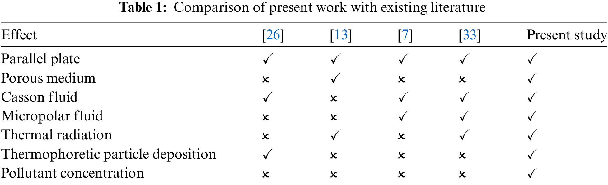
Ongoing through the literature survey, no work has been conducted to examine the mass and heat transmission analysis of Casson-micropolar liquid flow between a parallel plate in the presence of porous medium, T-R, TPD, and waste discharge concentration (see Table 1). The originality of our study is in the comprehensive examination of Casson micropolar fluid flow between parallel plates, incorporating crucial aspects such as waste discharge concentration, thermophoretic particle deposition, porous media, and thermal radiation-parameters that were not taken into account in prior research. In the present work, we utilize the RKF-45 scheme in combination with the shooting technique to efficiently handle the intricacies of highly nonlinear equations, resulting in accurate and dependable outcomes. This paper also presents the use of Artificial Neural Network methodology to enhance the precision of forecasts and optimize the analysis of parameters. New perspectives arising from the incorporation of environmental and thermal impacts greatly enrich the current body of knowledge. By acquiring knowledge of patterns in the parameter changes, the neural network facilitates the optimization of the solution process. The numerical outcomes are visualized concerning various parameters’ impact over different profiles, and important engineering factors are discussed in detail. Furthermore, our investigations provide practical applications in environmental management, namely in enhancing wastewater treatment and minimizing pollutants. Through a comprehensive analysis of thermophoretic effects and pollutant dynamics.

2  Mathematical Formulation

Consider the unsteady two-dimensional Casson micropolar fluid flow across two parallel plates in the existence of a permeable medium. The parallel plates are positioned at y=h(t)=l1−α2t and y=0. For α2<0, the plates are separated from each other, and for α2>0, both plates are compressed till they come into contact with each other at α2=t−1 (see Fig. 1). The temperature is denoted by the symbol T and concentration is denoted by the symbol C. Ch and Th corresponds to the concentration and temperature of the plate and Tw is the wall temperature. Further, thermal distribution within the fluid is modeled by including the impacts of thermal radiation and the concentration equation is modeled by external pollutant source and thermophoretic particle deposition.

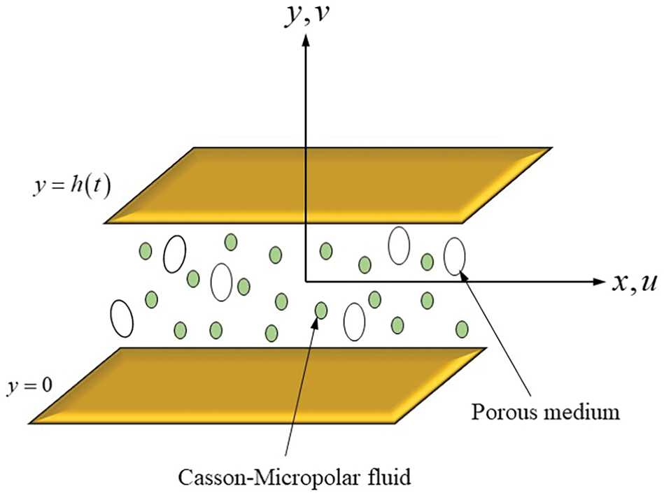
Figure 1: Flow diagram

The work of [34], specifically details the rheology of the Casson fluid model, providing the fundamental basis for the non-Newtonian behavior described. The non-newtonian model of Casson fluid is defined as (see [34])

Sij={2(μb+Py2Π)eij,Π>Πc,2(μb+Py2Πc)eij,Π>Πc.(1)

where, Π=eij.eij is the square of components of strain rate. Sij, μb, Py, and Πc are representing the components of (i,j)th Cauchy stress tensor, the dynamic viscosity of Casson fluid, yield stress, and critical value Π, respectively.

In developing the governing equations for the present study, previous literature provided a strong foundation. For instance, the research in [31], the paper examines the concentration of pollutants, while [35] investigates the dynamics of micropolar fluids between parallel surfaces. The Casson-Micropolar model is explored in [36], offering valuable insights, and [37,38] enhances our knowledge of the flow between parallel plates. Additionally, References [37] and [38] provide evidence for the representation of unstable or time-varying flows. Collectively, these sources provide a thorough basis for the development of the governing equations, and their combined perspectives were essential in generating the innovative elements of the present work.

The governing equations of the assumed flow are represented as follows (see for Eq. (7) [31], Eqs. (1)–(5) [35–38], Eq. (6) [39]):

∂u∂x=−∂v∂y,(2)

∂u∂t+v∂u∂y+u∂u∂x=−1ρf∂p∂x+(υf(1+1β)+Kρf)(∂2u∂x2+∂2u∂y2)−υfK∗u+Kρf∂N∂y,(3)

∂v∂t+u∂v∂x+v∂v∂y=−1ρf∂p∂y+(υf(1+1β)+Kρf)(∂2v∂x2+∂2v∂y2)+Kρf∂N∂y,(4)

∂N∂t+u∂N∂x+v∂N∂y=γρfj(∂2N∂x2+∂2N∂y2)−(2N+∂u∂y)Kρfj,(5)

∂T∂t+u∂T∂x+v∂T∂y=kf(ρCp)f(∂2T∂x2+∂2T∂y2)+1(ρCp)f16σ1∗T∞33k1∗(∂2T∂x2+∂2T∂y2),(6)

∂C∂t+u∂C∂x+v∂C∂y=Df(∂2C∂x2+∂2C∂y2)−∂(VTC)∂y+Q1exp⁡(b1C).(7)

The corresponding boundary circumstances are (see [33,39])

y=h(t):u=0,v=vw=dhdt,N=−ndudy,T=Tw,C=Ch,y=0:dudy=0,v=0,N=ndudy,∂T∂y=0,∂C∂y=0.}(8)

where, (u,v)-velocity components along the (x,y) directions. ρf-density, N-micro rotation component, υf-kinematic viscosity, kf-thermal conductivity, p-pressure, K-vertex viscosity, β-Casson parameter, Df-mass diffusivity, Cp-specific heat capacity, vw-mass transfer velocity, n-microrotation parameter, σ1∗-Stefan-Boltzmann coefficient, k1∗-mean absorption coefficient, VT-thermophoretic velocity, K∗-the permeability of the porous medium, b1-pollutant source external variation parameter, and Q1-external pollutant concentration.

In Eq. (5), the spin radiation viscosity is defined as (see [35])

γ=(μf+K2)j(9)

Here, μf-Dynamic viscosity, j is micro-inertia density, and it is given by j=υfα2(1−α2t).

And in Eq. (7), the thermophoretic velocity is (see [40])

VT=−k2υfTr∂T∂y.(10)

The Eq. (10), k2 represents the thermophoretic coefficient, Tr which represents the reference temperature.

Similarity variables are (see [39–41])

η=yl(1−α2t)12,u=α2x2(1−α2t)f′,v=−α2l2(1−α2t)12f,N=α2x2l(1−α2t)32ϕ(η),θ(η)=T−ThTw−Th,χ(η)=CCh.}(11)

Using Eq. (11), the Eq. (2) is identically satisfied. The pressure term is eliminated from the governing Eqs. (3) and (4) and takes the form of Eq. (12). Further, the Eqs. (5)–(7) will be reduced to Eqs. (13)–(15), respectively.

((1+1β)+K1)f′′′′−λ1f′′+K1ϕ′′−S1(ηf′′′+3f′′+f′f′′−ff′′′)=0,(12)

(1+K12)ϕ′′−2K1S1(2ϕ+f′′)−S1(ηϕ′+3ϕ+ϕf′−fϕ′)=0,(13)

θ′′+43Rθ′′+PrS1(fθ′−ηθ′)=0,(14)

χ′′−Scτ(χθ′′+θ′χ′)+Scδ∗exp⁡(σ∗χ)−ScS1(ηχ′−fχ′)=0.(15)

Boundary conditions (BCs) are reduced to the following form:

η=1:f′(1)=0,ϕ(1)=−nf′′(1),f(1)=1,χ(1)=1,θ(1)=1,η=0:f′′(0)=0,f(0)=0,ϕ(0)=nf′′(0),θ′(0)=0,χ′(0)=0.}(16)

From the Eqs. (12) to (16), non-dimensional parameters are

K1—micropolar parameter S1—Squeeze number Pr—Prandtl number

λ1—porous parameter R—radiation parameter Sc—Schmidt number

σ∗—external pollutant source variation parameter

τ—thermophoretic parameter

δ∗—local pollutant external source parameter.

K1=Kμf,S1=α2l22υf,λ1=l2(1−α2t)K∗,Pr=μf(Cp)fkf,R=4σ∗T∞3k1∗kf,σ∗=b1Ch,δ∗=Q1l2(1−α2t)Chυf,Sc=υfDf,τ=−k2Tr(Tw−Th).}(17)

Special Cases:

a) If β>0 the model becomes Casson-micropolar fluid flow.

b) If β→∞, the model becomes micropolar fluid flow.

Some important Engineering coefficients are (see [13,42])

Skin friction:

Cf∗=1ρfvw2(μf(1+1β)+K)∂u∂y|y=h(t).(18)

The reduced form of Eq. (18) is

Cf=l2x2(1−α2t)12Cf∗=1Rex((1+1β)+K1)f′′(1).(19)

where, Rex=α2lx2υf (Local Reynolds number)

Nusselt number:

Nu∗=−l(Tw−Th)kf(kf∂T∂y+16σ1∗T∞33k1∗∂T∂y)|y=h(t).(20)

The reduced form of Eq. (20) is

Nu=(1−α2t)Nu∗=−(1+43R)θ′(1).(21)

Sherwood number:

Sh∗=−lChDf(Df∂C∂y)|y=h(t).(22)

Eq. (22) is reduced to the following form:

Sh=(1−α2t)Sh∗=−χ′(1).(23)

3  Numerical Procedure

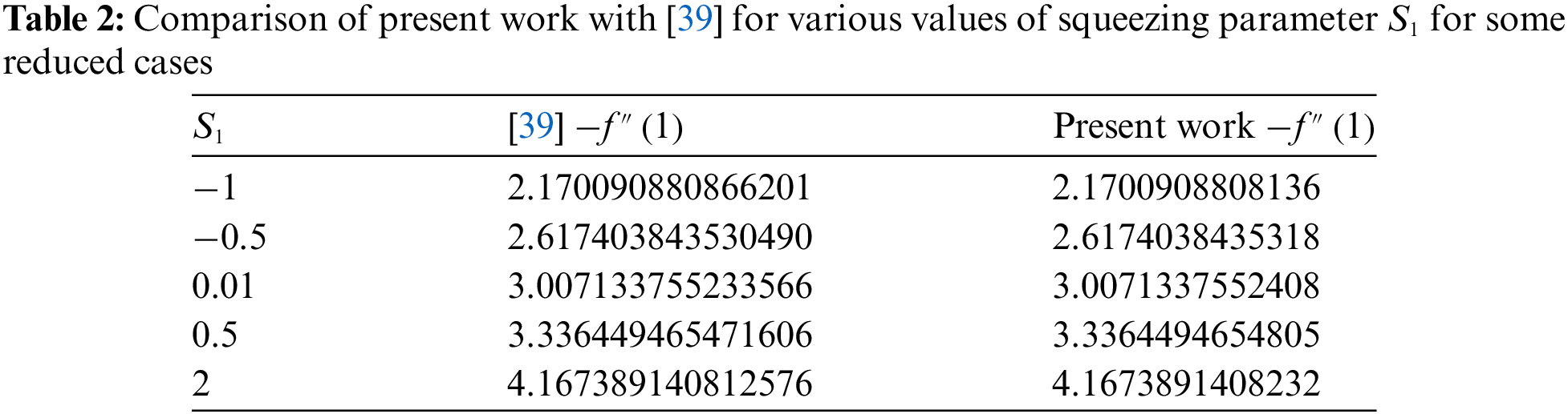
The reduced Eqs. (12)–(15) and BCs (16) are solved numerically utilizing the RKF-45 and a shooting approach due to the presence of higher order and two-point boundary. Obtaining the analytical solution is too difficult for these kinds of problems. Hence, to obtain the solutions, the first step is to make them in a first-order equation form. For this process, the following substitutions are used.

Let us choose, {f,f′,f′′,f′′′,ϕϕ′,θ,θ′,χ,χ′}≃{g1,g2,g3,g4,g5g6,g7,g8,g9,g10}(24)

f′′′′=−[−λ1g3+K1[R.H.Sofeqn.(25)]−S1(ηg4+3g3+g2g3−g1g4)]((1+1β)+K1)−1(25)

ϕ′′=−[−2K1S1(2g5+g3)−S1(ηg6+3g5+g5g2−g1g6)](1+K12)−1,(26)

θ′′=−PrS1(g1g8−ηg8)(1+43R)−1,(27)

χ′′=−[−Scτ(g9(−PrS1(g1g8−ηg8)(1+43R)−1)+g8g10)+Scδ∗exp⁡(σ∗g9)−ScS1(ηg10−g1g10)].(28)

Boundary conditions become

g2(1)=0,g5(1)=−ng3(1),g1(1)=1,g9(1)=1,g7(1)=1,g3(0)=0,g1(0)=0,g5(0)=ng3(0),g8(0)=0,g10(0)=0.}(29)

The converted equations are now solved by using the RKF-45 and the shooting scheme is used to find the values of unknown boundary conditions present in the equation number (29) such as g4(0)=δ1&g6(0)=δ2. The values of δ1 and δ2 are chosen in such a way that it should meet the boundary conditions at η=1. Further, in g5(1)=−ng3(1) condition in which g5(1) is depends on g3(1). The term g3(1) with the product of n is further treated as an additional variable δ3 and its value should be obtained by a shooting scheme. As mentioned above, a similar strategy is applied to find the value of δ3. Based on the obtained guessings for all the three unknowns, the boundary conditions g4(0), g6(0) and g5(1)=−ng3(1) should be satisfied. If these guesses don’t satisfy the boundary conditions, adjustments will be made. By setting the step size to 0.01 and the error tolerance about 10−6. This shooting method works iteratively and is based on guessing, integration, and checking the boundary conditions until the prescribed error tolerance is met. The values of the parameters are selected to demonstrate the distinct influence of each parameter. In addition, error tolerance has been acquired for each iteration, and numerical outcomes are displayed via graphs. The present numerical approach has been validated by associating it with existing work, and its findings show a strong agreement (refer to Table 2).

The numerical flowchart of the current scheme is shown in Fig. 2. The solution algorithm to solve the given system of reduced equations and boundary conditions is given below.

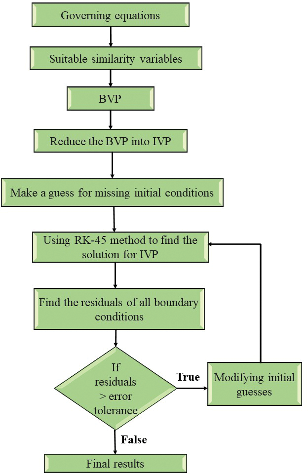
Figure 2: Numerical flow chart

3.1 Solution Algorithm

Initialization:

•   Define the initial and BCs (29) for the variables g3,g1,g5,g8,g10 at η=0.

•   Set the range of independent variable η from zero to one.

Substitution:

•   Substitute the following variables:

f=g1,f′=g2,f′′=g3,f′′′=g4,ϕ=g5,ϕ′=g6,θ=g7,θ′=g8,χ=g9,χ′=g10.

•   Transform the fourth-order and second-order ODEs into first-order ODEs by employing these substitutions.

System of first-order ordinary differential equations:

•   Compute the first-order system of equations and give the values for all the parameters.

•   Apply the BCs to the first-order ODEs.

Numerical solver:

•   The shooting scheme is used to find the unknown values of the boundary conditions. The values obtained during the shooting procedure are used to solve the system of equations. The solution of these equations is compared with the boundary conditions. The initial guesses are chosen in such a way that they should meet the error tolerance criteria and boundary conditions at the endpoint. The unknown boundary conditions present in the resultant equations such as g4(0),g6(0) and g5(1)=−ng3(1) are obtained using the shooting scheme such that it should meet the boundary conditions at η=1.

•   Using MATLAB and RKF-45, the following transformed system of equations and BCs can be implemented, with the step size set to 0.01 and the error tolerance set to roughly 10−6.

The process described above outlines the step-by-step computing approach to solve the system of equations and BCs numerically. When an approach is incorporated into the research, understanding of the sequence in which the equations are solved will be improved, ensuring that the method can be repeated and understood.

4  Results and Discussion

This section explores the impact of various dimensionless parameters (porous parameter, micropolar parameter, radiation parameter, thermophoretic parameter, local pollutant external source parameter, and external pollutant source variation). The effects of these elements are examined using graphical evaluation, which offers a deeper understanding of how they influence the velocity, temperature, and concentration profiles in the liquid. In addition, the discussion emphasizes the importance of these parameters in engineering applications by examining key factors such as skin friction, Nusselt number, and Sherwood number. Such coefficients are crucial for assessing the properties of both mass and heat transmission. This thorough analysis provides a more profound comprehension of the motion of fluids and dispersion of pollutants in the system, which assists in the creation of more efficient solutions for environmental management. The considered parameter ranges are: λ1 [1–20], K1 [1–10], n [0.1–1], R [1–5], τ [0.1–0.5], δ∗ [0.1–0.5], and σ∗ [0.1–0.5]. Here, the range of the parameters was selected based on the previous studies to obtain a clear variation and the influence of the pertinent parameters on the involved profiles.

Fig. 3 represents the impact of λ1 on f′(η) for both cases (β=0.5 and β→∞). As the λ1 value increases, velocity increases for 0.4≥η≥1 (upper plate) and decreases for 0≤η≤0.4 (lower plate). From a physical standpoint, this implies that the impedance of the porous substance has varying effects on the movement of the liquid at different locations across the plates. In the Casson-micropolar liquid, the velocity decreases substantially closer to the lower plate due to the impedance caused by its yield stress properties. Conversely, closer to the upper plate, the velocity boosts greater in the micropolar fluid, possibly because of its microstructure and rotation consequences that conquer the opposition of the porous medium.

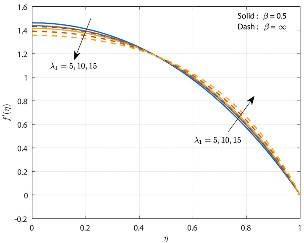
Figure 3: Effect of porous parameter on velocity profile

Fig. 4 exemplifies the effect of K1 on f′(η) for both cases (β=0.5 and β→∞). As the K1 value increases, velocity increases for 0≤η≤0.4 and decreases for 0.4≥η≥1. This suggests that the micropolar parameter, which accounts for the micro-rotational effects and the fluid’s microstructure, enhances fluid momentum close to the lower plate by reducing the resistance to flow. Near the upper plate, these rotational processes exert a significant influence, resulting in a decrease in velocity. The increased velocity in the micropolar liquid close to the top plate can be explained by its capacity to incorporate these micro-rotational consequences, whereas the Casson-micropolar liquid, due to its yield stress features, sustains a higher velocity towards the lower plate.

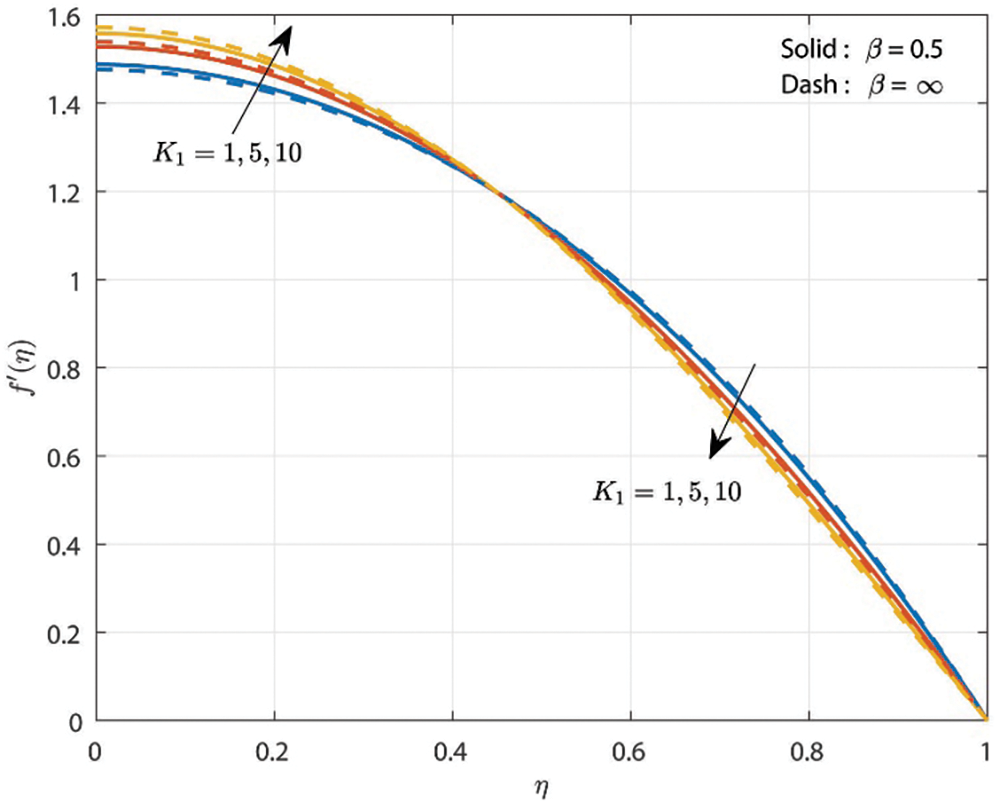
Figure 4: Effect of micropolar parameter on velocity profile

The effect of K1 on the microrotation velocity profile ϕ(η) is represented in Fig. 5. Here, the increase in the value of K1, the ϕ(η) profile is also increasing for both β=0.5 and β→∞. As the micropolar parameter, the microrotation velocity profile likewise grows, suggesting that the intensified micro-rotational impacts magnify the rotational motion of fluid particles. The enhancement in ϕ(η) is more prominent in the micropolar liquid than in the Casson-micropolar liquid. This difference might be due to the presence of yield stress in the Casson liquid, which limits rotational movement until a specific threshold is surpassed. The increased microrotation velocity in the micropolar liquid indicates its enhanced capacity to tolerate rotational impacts, rendering it more sensitive to the micropolar component.

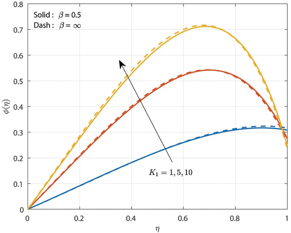
Figure 5: Effect of micropolar parameter on the micro rotation velocity profile

Fig. 6 shows the consequence of K1 on θ(η) for β=0.5 and β→∞. For both β=0.5 and β→∞, the θ(η) profile is rising with increased values of K1, and the temperature at β→∞ is higher than it is at β=0.5. The physical explanation for this phenomenon lies in the distinctive properties of micropolar liquids, which exhibit micro-rotational effects and coupling tensions. These features enable more efficient energy transfer within the liquid, resulting in better thermal conduction and a more even distribution of heat. In the absence of β, the temperature is seen to be higher than when it is present. The β, which characterizes the yield stress behavior in non-Newtonian liquids, adds extra opposition to the flow. The presence of β reduces the fluid’s efficiency in transferring heat, foremost to a decrease in the θ(η). Hence, the correlation among the β and K1 parameters substantially impact the liquid’s thermal characteristics.

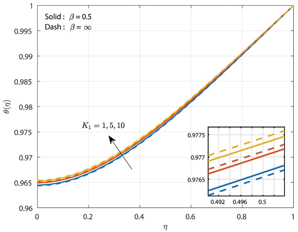
Figure 6: Effect of micropolar parameter on temperature profile

The nature of K1 on χ(η) is represented in Fig. 7. The increase in K1 improves the concentration for both cases β=0.5 and β→∞. The concentration is more in the presence of β than its absence in the presence of K1. In the absence of β, the concentration is seen to be decreased in comparison to its existence. The concentration in the micropolar fluid is greater than that in the Casson-micropolar fluid, most likely because the latter has a yield stress that limits the dispersion of particles until a critical stress level is achieved.

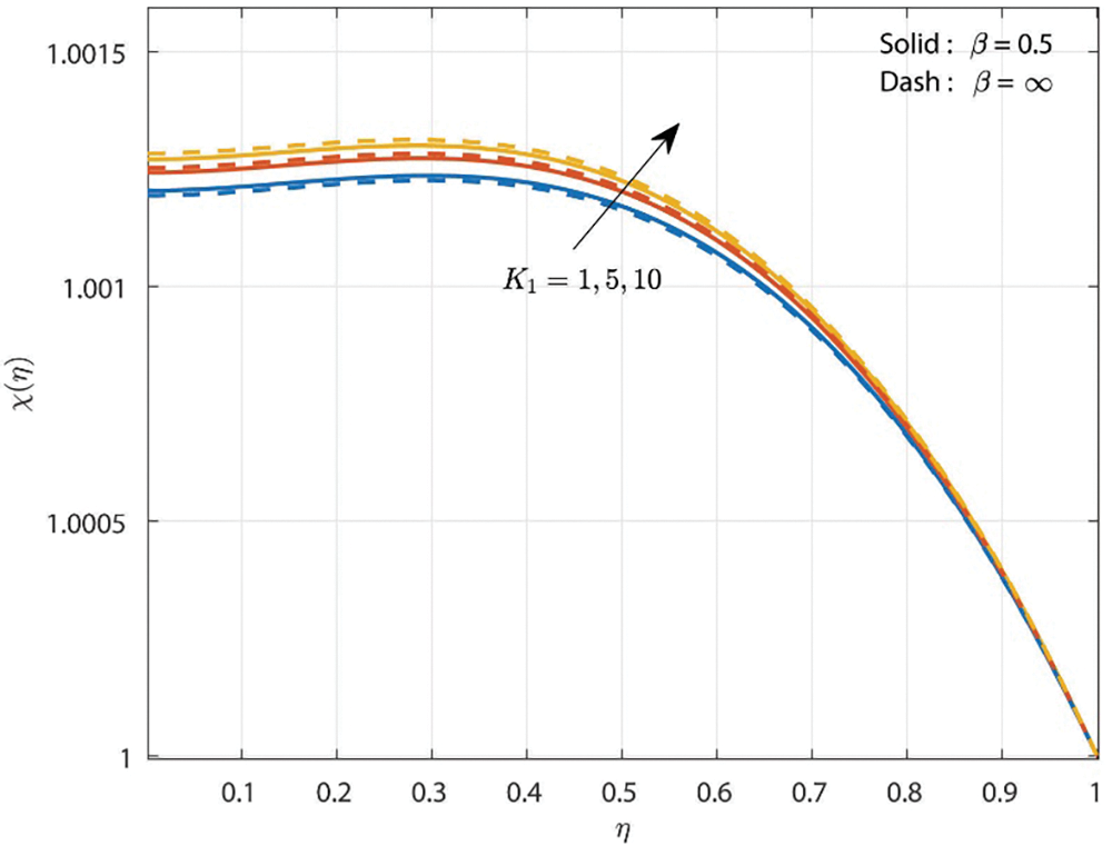
Figure 7: Effect of micropolar parameter on concentration profile

In Fig. 8, the influence of n on the micro rotation ϕ(η) is explained. For both cases (β=0.5 and β→∞), a rise in n leads to an enhancement in the ϕ(η). When the microrotation parameter rises, the microrotation velocity profile similarly grows, suggesting that stronger rotational influences enhance the rotational velocity of liquid particles. The boost in rotational motion is more significant in micropolar fluids than in Casson-micropolar fluids, primarily because the yield stress of the Casson fluid restricts rotational motion until a particular limit is surpassed.

Figure 8: Effect of microrotation parameter on the micro rotation velocity profile

The outcome of R on θ(η) is explained in Fig. 9. A rise in R upsurges the temperature for β=0.5 and β→∞. The thermal distribution rate is greater in the case of β=0.5 compared to the case β→∞. Physically, as the radiation parameter increases, the temperature profile also goes up, suggesting that more thermal radiation improves heat transport inside the liquid. The impact is more pronounced in the Casson-micropolar liquid as opposed to the micropolar liquid. The elevated temperature observed in the Casson-micropolar fluid can be ascribed to its yield stress properties, which impede fluid movement and result in increased heat accumulation. On the other hand, the micropolar fluid, due to its fundamental micro-rotational properties, enhances heat dissipation, leading to a comparatively reduced temperature profile.

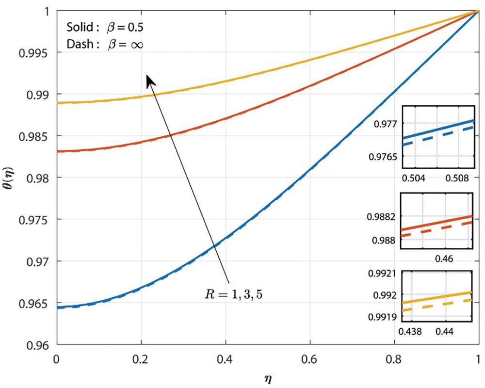
Figure 9: Effect of radiation parameter on temperature profile

Fig. 10 describes how τ affects the χ(η) profile for both cases (β=0.5 and β→∞). The thermophoretic parameter significantly influences the concentration profile. An increase in τ concentration decreases for both cases β=0.5 and β→∞. As the thermophoretic parameter increases, the concentration profile lowers due to the effect of thermophoresis. Thermophoresis induces molecules to migrate from heated to colder locations, resulting in a reduction of concentration in regions with greater temperatures. The drop is particularly noticeable in micropolar fluids, possibly because of their heightened micro-rotational effects that aid in the dispersal of particles. On the other hand, the Casson-micropolar fluid demonstrates a greater concentration profile due to its ability to oppose the swirling of particles through its yield stress, resulting in a more condensed dispersion.

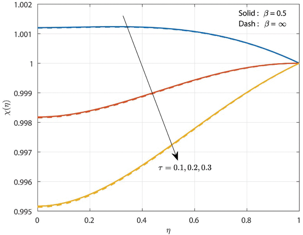
Figure 10: Effect of thermophoretic parameter on concentration profile

Fig. 11 illustrates the effect of δ∗ impacts the χ(η) profile. With an increase in δ∗ the χ(η) profile increases for both β=0.5 and β→∞. Physically, the fluid concentration improves when δ∗ gets improved because more liquid will be involved in the liquid flow throughout the region. The χ(η) profile improves with an rise in δ∗. The magnitude of this impact is more noticeable in the micropolar liquid as compared to the Casson-micropolar liquid. The increased concentration in the micropolar fluid can be ascribed to its micro-rotational phenomena, which facilitate enhanced dissemination and connection to the external source of contaminants. The Casson-micropolar fluid, due to its yield stress, limits the mobility of particles, resulting in a comparatively lower concentration profile.

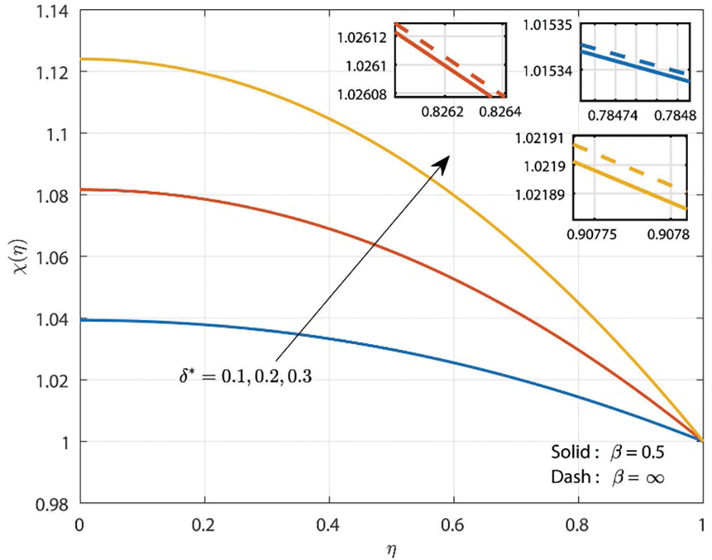
Figure 11: Effect of local pollutant external source parameter on concentration profile

Fig. 12 illustrates how the σ∗ impacts on χ(η) profile. The χ(η) escalates with a rise in the σ∗ for both β=0.5 and β→∞. δ∗ and σ∗ both possess almost similar functions and these two parameters are relevant to the amount of pollutants introduced into the flow. The increased concentration in the Casson-micropolar liquid can be ascribed to its yield stress, which diminishes fluid movement and thus facilitates the accumulation of contaminants. On the other hand, the micropolar fluid, due to its micro-rotational properties, enhances the distribution of contaminants, resulting in a comparatively reduced concentration profile. This distinction is noteworthy in the field of handling the environment and manufacturing operations since it is crucial to regulate the levels of pollutants.

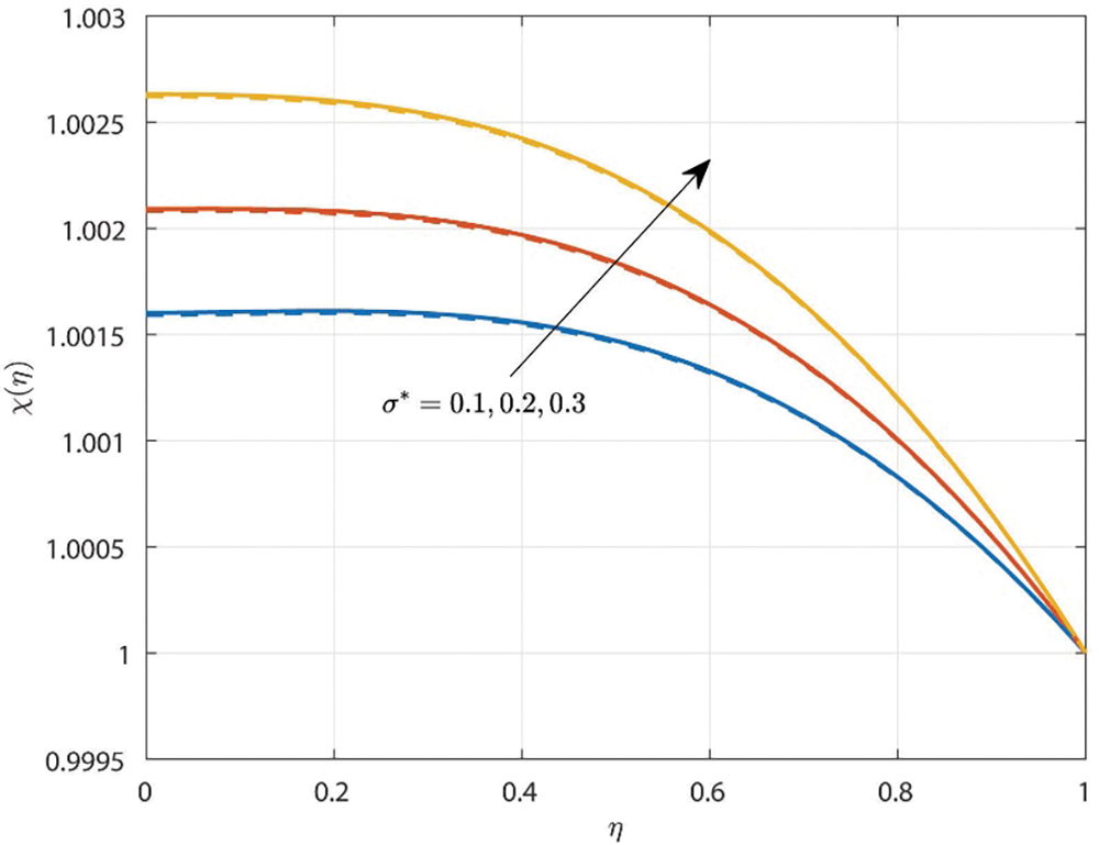
Figure 12: Effect of external pollutant source variation parameter on concentration profile

Fig. 13 shows the influence of K1 on Cf vs. λ1 for both β=0.5 and β→∞ cases. Here, the increase in values of K1 and λ1 declines the surface drag force for both β=0.5 and β→∞ cases. However, in this case β=0.5, the surface drag force is lower than in the case β→∞. The rise in K1 amplifies the micro-rotational impacts and coupling stresses present in the micropolar liquid, resulting in decreased shear forces at the outermost layer. Similarly, an increased value of λ1 indicates a higher level of penetration in a porous substance, which leads to a stronger connection between the liquid and its outer layer, resulting in a decrease in Cf. Further, for β=0.5, the liquid experiences lesser resistance which results in higher shear stress resulting in lower Cf than β→∞.

Figure 13: Effect of micropolar parameter on skin friction vs. porous parameter

Fig. 14 shows the influence of K1 on Nu vs. R for both β=0.5 and β=∞ cases. Here, the increase in values of K1 and R will increase the heat transmission rate for both cases (β=0.5 and β→∞). It is noted that the rate of heat transmission is greater in the case β→∞ compared to the case β=0.5. The rise in K1 declines energy transfer processes by enhancing micro-rotational effects and coupling tensions in the micropolar fluid, hence facilitating less thermal conduction. Moreover, a larger R indicates an augmented emission T-R, hence enhancing the total heat transfer rate through facilitating a greater interchange of energy among the liquid and its surrounding environment which results in less Nu. For β=0.5 the liquid demonstrates increased viscosity, thereby impeding effective thermal conduction than β→∞.

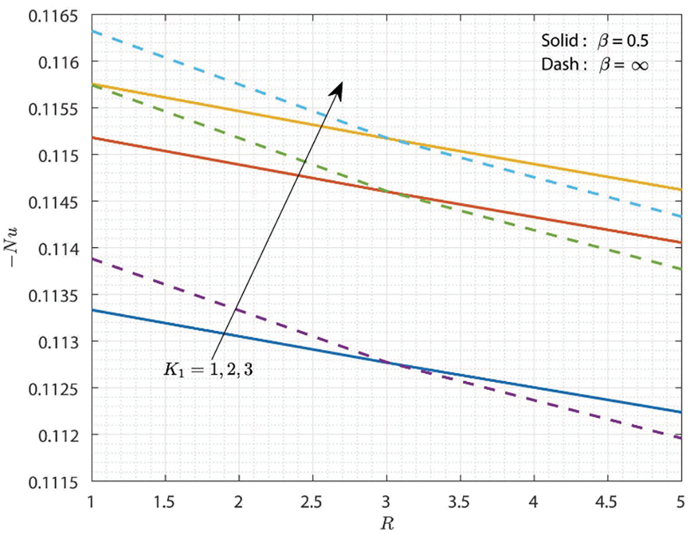
Figure 14: Effect of micropolar parameter on Nusselt number vs. radiation parameter

Fig. 15 shows the influence of K1 on Sh vs. δ∗ for both β=0.5 and β→∞ cases. Here, the increase in values of K1 and δ∗ upsurges the rate of mass transmission for both cases (β=0.5 and β→∞). However, the mass transfer rate is greater in the case β=0.5 compared to the case β→∞. The rise in K1 amplifies the micro-rotational processes and couples tensions within the micropolar liquid, resulting in improved mass transfer performance. Moreover, a greater δ∗ signifies a more potent external origin of contaminants, thereby amplifying the concentration difference and propelling a larger rate of mass movement. The rate of mass movement is higher when β=0.5 than when β→∞.

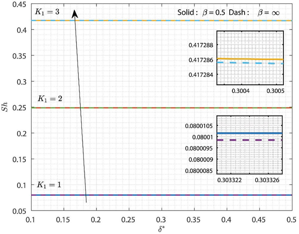
Figure 15: Effect of micropolar parameter on Sherwood number vs. local pollutant external source parameter

5  Application of Artificial Neural Network (ANN): Levenberg-Marquardt (LM) Backpropagation Technique

Neural networks are highly effective for simulating mathematical models and excel at predicting their outcomes. One such network is a Multi-Layer Perceptron (MLP) with Levenberg-Marquardt (LM) backpropagation. LM backpropagation technique is one of the powerful optimization methods used for solving non-linear problems. This scheme was first introduced by the mathematician Kenneth Levenberg in the year 1944. His work is mainly carried out to improve the efficiency of least-squares minimization techniques, particularly for nonlinear systems. Later it was rediscovered by the scientist Donald Marquardt in the year 1963. Marquardt first built upon Levenberg’s work in refining the algorithm to produce more efficient and stable performance. With his enhancements, the method could find a way to adaptively toggle between two optimization strategies (Gauss-Newton and gradient descent) depending on problem characteristics at every iteration. The LM backpropagation algorithm quickly gained extensive attention as it showed fast convergence and reliable results so it is widely applied to many areas of science and engineering. The architecture of MLP proposed in this work is shown in Fig. 16.

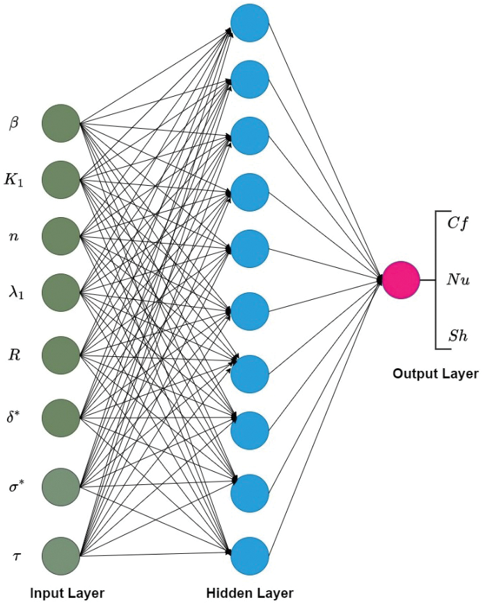
Figure 16: Geometry of the MLP-proposed model

The proposed model contains mainly three components namely, input layer, hidden layer, and output layer. The input layer is called the first layer of the ANN model, such that it acts as an entry point to the data into the neural network model. This layer forwards the data to the next layer called the hidden layer without any processing. In the input layer, the number of neurons is equivalent to the number of input (Ii) components i.e., β,K1,n,λ1,R,δ∗,σ∗,&τ. The second layer called the hidden layer performs computation on the data taken by the input layer by implementing the weights, biases, and activation function. The data set is generated by the proposed numerical scheme (RKF-45 and Shooting scheme) in Section 3. The data set is generated for engineering factors such as Cf,Nu&Sh. About 2376 samples are generated in a combination of these engineering factors and this is considered as the dataset for the neural network model. The data is divided into 70:20:10 for training, testing, and validation purposes. During training, for each sample in the dataset, the inputs (Ii) are multiplied with the corresponding weights (wji) and the weighted sum of inputs (Oj) is generated by using Eq. (30), where b is the bias at each neuron.

Oj=∑i=1nwji•Ii+bj.(30)

An activation function (LeakyReLU) is applied to this weighted sum to generate the output using Eq. (31).

YANN=LeakyReLU(Oj)={OjifOj≥0ω•OjifOj<0.(31)

Then based on the difference between the generated and desired output the LM algorithm adjusts the weights and biases. This process continues till the error between the neural network-generated outputs and the desired outputs for the entire training dataset is minimal. During testing, the trained model predicts the output by using Eq. (31). The MSE (mean square error) and R2 (Coefficient of determination) are chosen to evaluate the prediction effectiveness. The mathematical formula for MSE and R2 is given below (see (32) and (33)):

MSE=1K∑i=1K(YRKF−45(i)−YANN(i))2.(32)

where, K signifies the number of data points, YRKF−45 is the observed values of Cf,Nu&Sh, YANN is the predicted values of Cf,Nu&Sh.

R2=1−∑i=1K(YRKF−45(i)−YANN(i))2∑i=1K(YRKF−45(i))2.(33)

where, ∑i=1K(YRKF−45(i)−YANN(i))2 denotes the sum of squares of residuals and ∑i=1K(YRKF−45(i))2 is the total sum of squares.

Fig. 17a shows the validation performance for the output variables Cf,Nu&Sh. From the figure it is observed that mean square error MSE values show high at the beginning for both testing, training, and validation for the present ANN scheme but during increasing the epochs process, all three processes are attaining their optimum state, and the best fit is observed. During this state, the mean square error falls within the best-fit line. The ANN models take the training phase to calculate the zero error for mean square error and it was found that 2.4427e−10 at the epoch of 509. Further, the error histogram of the overall model is displayed in Fig. 17b. These histograms display the statistical distribution of errors for each expected value, beginning with a zero-error point and progressing upwards. Errors are classified into 20 distinct bins and then organized in a row along a linear segment known as the zero-error line. Greater proximity of data to the zero-error line will be observed in a solution approach that exhibits higher levels of accuracy and precision. It is observed that zero error for overall data is 2.21e−6.

Figure 17: (a) Performance plot of ANN, (b) Error histogram

An essential tool for assessing the effectiveness of a neural network model trained with the Levenberg-Marquardt (LM) backpropagation approach is a regression chart. This metric graphically illustrates the degree of agreement between the projected outcomes of the model and the real data for training, testing, validation, and overall efficacy. A regression plot of the current analysis of the data is shown in Fig. 18. From the figure it is seen that there are four regression subplots such as training, testing, validation, and overall. In the training plot, it is seen that there is a linear relationship between the data. The training plot claims that the present model is well-fitted for the training phase. Furthermore, the validation regression plot indicates that the model has acquired specific patterns from the training data rather than generalized patterns. The testing regression plot shows an excellent correspondence between the observed and projected values in this case validates the model’s resilience and ability to generalize. Lastly, the overall regression plot facilitates the comparison of outcomes throughout the several phases of the modeling approach and guarantees uniformity.

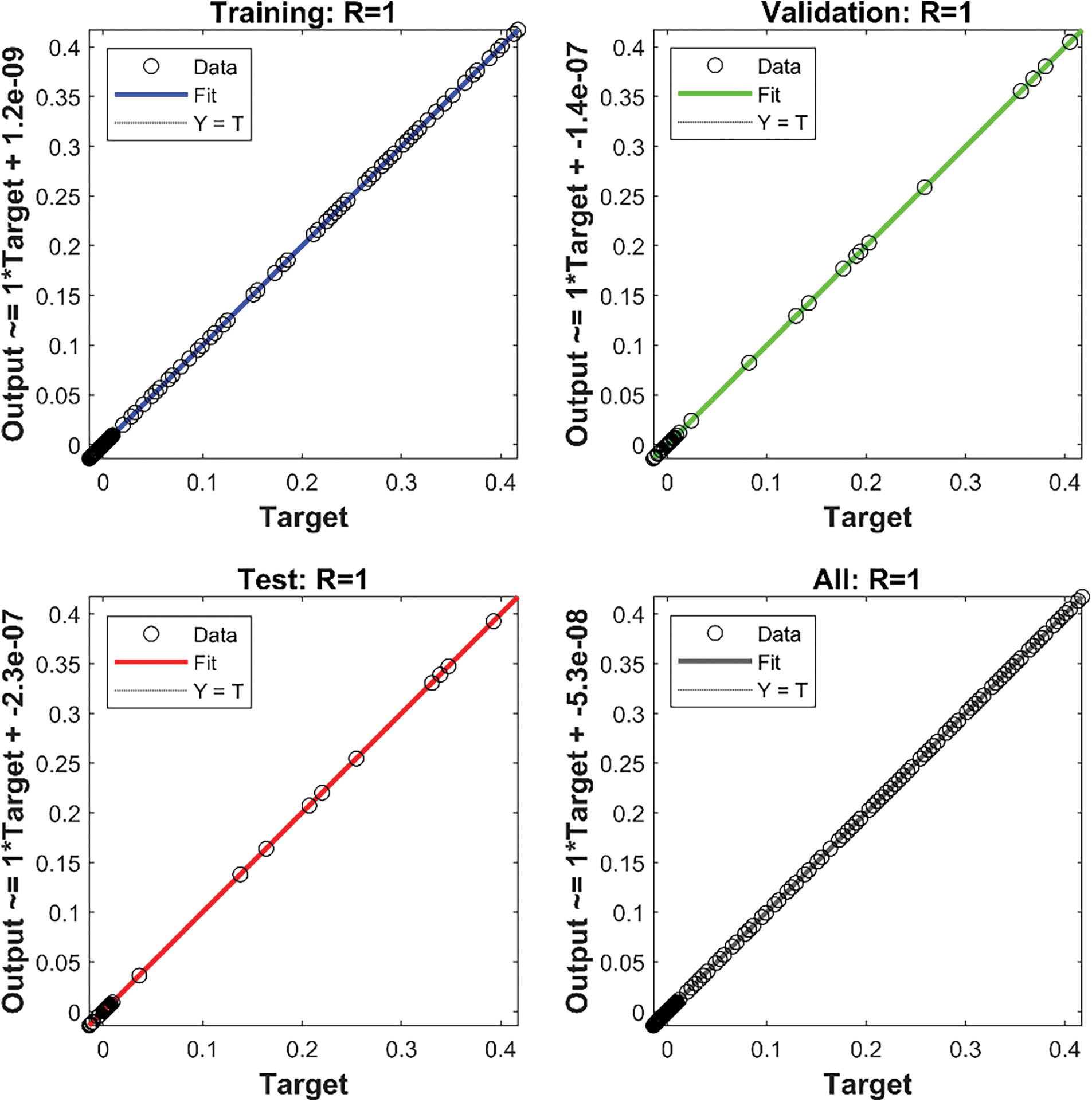
Figure 18: Pictorial representation of regression plot for output and predicted values

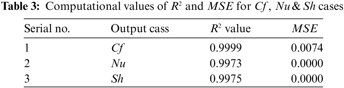
The individual computational values of R2 and MSE for all three cases are provided in Table 3. It is observed that the data is closely co-related and the mean square error is near zero in Cf case and zero in the other two cases.

6  Conclusion

The current study explores the time-dependent two-dimensional stream of Casson micropolar fluid through parallel surfaces under the effect of porous media, T-R, TPD, and waste discharge concentration. The governing equations are reduced to ODEs with the help of suitable similarity transformations. The RKF-45 and shooting procedure are utilized to solve the reduced set of equations and boundary conditions numerically. The major findings of the study are given below:

➢   The velocity declines at the lower plate and enhances at the upper plate due to an increase in the values of porous constraint while reverse behavior is seen in the case of micropolar parameter.

➢   The increase in the values of micropolar parameters will enhance microrotation, temperature, and concentration profiles.

➢   The upsurge in the values of the thermal radiation parameter will increase the temperature profile.

➢   Augmented values of thermophoretic constraint will decline the concentration while local and external pollutant sources will enhance the concentration.

➢   The improvement in micropolar and porous parameters will reduce the surface drag force.

➢   In major cases, micropolar fluid outperforms Casson-micropolar liquid.

➢   The ANN models achieve the best performance of 2.4427e−10 for Cf,Nu&Sh at epoch of 509.

➢   The training, testing, validation, and overall performance are obtained by regression plots and the best fit of data is observed in all these phases.

The present study is limited to examining the stream of Casson micropolar fluid through parallel surfaces under the effect of porous media, T-R, TPD, and waste discharge concentration. The present work can be extended to examine the various kinds of non-Newtonian fluids, different kinds of nanofluid models, various types of physical constraints, and different boundary conditions.

Acknowledgement: This work was supported and funded by the Deanship of Scientific Research at Imam Mohammad Ibn Saud Islamic University (IMSIU).

Funding Statement: We would like to thank the Deanship of Scientific Research at Imam Mohammad Ibn Saud Islamic University (IMSIU) for paying the open access fees.

Author Contributions: The authors confirm their contribution to the paper as follows: study conception and design: Ghaliah Alhamzi, Vinutha Kalleshachar, Badr Saad T. Alkahtani; data collection: Vinutha Kalleshachar, Badr Saad T. Alkahtani; analysis and interpretation of results: Vinutha Kalleshachar, Ravi Shanker Dubey, Badr Saad T. Alkahtani; draft manuscript preparation: Vinutha Kalleshachar, Neelima Nizampatnam, Ghaliah Alhamzi. All authors reviewed the results and approved the final version of the manuscript.

Availability of Data and Materials: The data are available from the corresponding author on reasonable request.

Ethics Approval: Not applicable.

Conflicts of Interest: The authors declare no conflicts of interest to report regarding the present study.

References

1. Ismael AM, Eldabe NT, Zeid MYA, Shabouri SME. Thermal micropolar and couple stresses effects on peristaltic flow of biviscosity nanofluid through a porous medium. Sci Rep. 2022;12(1):16180. doi:10.1038/s41598-022-20320-6. [Google Scholar] [PubMed] [CrossRef]

2. Yasir M, Bilal S, Ahammad NA, Elseesy IE. Thermal irregular generation and absorption of nanoscale energy transportation of thermodynamic material of a micropolar fluid. Ain Shams Eng J. 2024;15(9):102948. doi:10.1016/j.asej.2024.102948. [Google Scholar] [CrossRef]

3. Siddiqui AA, Turkyilmazoglu M. Slit flow and thermal analysis of micropolar fluids in a symmetric channel with dynamic and permeable. Int Commun Heat Mass Transf. 2022;132:105844. doi:10.1016/j.icheatmasstransfer.2021.105844. [Google Scholar] [CrossRef]

4. Ram MS, Spandana K, Shamshuddin MD, Salawu SO. Mixed convective heat and mass transfer in magnetized micropolar fluid flow toward stagnation point on a porous stretching sheet with heat source/sink and variable species reaction. Int J Model Simul. 2022;43(5):670–82. doi:10.1080/02286203.2022.2112008. [Google Scholar] [CrossRef]

5. Siddiqui AA, Turkyilmazoglu M. Film flow of nano-micropolar fluid with dissipation effect. Comput Model Eng Sci. 2024;140(3):2488–9. doi:10.32604/cmes.2024.050525. [Google Scholar] [CrossRef]

6. Li P, Duraihem FZ, Awan AU, Al-Zubaidi A, Abbas N, Ahmad D. Heat transfer of hybrid nanomaterials base maxwell micropolar fluid flow over an exponentially stretching surface. Nanomaterials. 2022;12(7):1207. doi:10.3390/nano12071207. [Google Scholar] [PubMed] [CrossRef]

7. Shamshuddin MD, Ibrahim W. Finite element numerical technique for magneto-micropolar nanofluid flow filled with chemically reactive casson fluid between parallel plates subjected to rotatory system with electrical and Hall currents. Int J Model Simul. 2022;42(6):985–1004. doi:10.1080/02286203.2021.2012634. [Google Scholar] [CrossRef]

8. Shamshuddin MD, Mabood F, Khan WA, Rajput GR. Exploration of thermal Péclet number, vortex viscosity, and Reynolds number on two-dimensional flow of micropolar fluid through a channel due to mixed convection. Heat Transfer. 2022;52(1):854–73. doi:10.1002/htj.22719. [Google Scholar] [CrossRef]

9. Yasir M, Khan M, Al-Zubaidi A, Saleem S. Arrhenius activation energy effect in thermally viscous dissipative flow of micropolar material with gyrotactic microorganisms. Alex Eng J. 2023;84:204–14. doi:10.1016/j.aej.2023.11.003. [Google Scholar] [CrossRef]

10. Muntazir RM, Mushtaq M, Shahzadi S, Jabeen K. MHD nanofluid flow around a permeable stretching sheet with thermal radiation and viscous dissipation. Proc Inst Mech Eng C J Mech Eng Sci. 2021;236(1):137–52. doi:10.1177/09544062211023094. [Google Scholar] [CrossRef]

11. Salawu SO, Obalalu AM, Fatunmbi EO, Shamshuddin M. Elastic deformation of thermal radiative and convective hybrid SWCNT-Ag and MWCNT-MoS4 magneto-nanofluids flow in a cylinder. Results Mater. 2023;17:100380. doi:10.1016/j.rinma.2023.100380. [Google Scholar] [CrossRef]

12. Famakinwa OA, Koriko OK, Adegbie KS, Omowaye AJ. Effects of viscous variation, thermal radiation, and Arrhenius reaction: the case of MHD nanofluid flow containing gyrotactic microorganisms over a convectively heated surface. Partial Differ Equ Appl Math. 2021;5:100232. doi:10.26565/2312-4334-2023-4-10. [Google Scholar] [CrossRef]

13. Mohamed Y, Eldabe N, Abouzeid M, Mostapha D, Ouaf M. Chemical reaction and thermal radiation via Cattaneo-Christov double diffusion (CCDD) effects on squeezing non-Newtonian nanofluid flow between two-parallel vertical plates. Egypt J Chem. 2022;26(3):209–31. doi:10.21608/ejchem.2022.145286.6332. [Google Scholar] [CrossRef]

14. Fatunmbi EO, Okoya SS. Nonlinear radiative thermal analysis of magneto-micropolar fluid over a bidirectionally extending sheet with varied thermal conditions. Case Stud Therm Eng. 2024:104712. doi:10.1016/j.csite.2024.104712. [Google Scholar] [CrossRef]

15. Zhang K, Shah NA, Alshehri M, Alkarni S, Wakif A, Eldin SM. Water thermal enhancement in a porous medium via a suspension of hybrid nanoparticles: MHD mixed convective Falkner’s-Skan flow case study. Case Stud Therm Eng. 2023;47:103062. doi:10.1016/j.csite.2023.103062. [Google Scholar] [CrossRef]

16. Zheng K, Shah SI, Khan MN, Tag-Eldin E, Yasir M, Galal AM. Numerical simulation of melting heat transfer towards stagnation point region over a permeable shrinking surface. Sci Iran. 2022. doi:10.24200/sci.2022.59956.6518. [Google Scholar] [CrossRef]

17. Hiremath P, Hanumagowda BN, Subray PVA, Sharma N, Varma SVK, Muhammad T, et al. Sensitivity analysis of MHD nanofluid flow in a composite permeable square enclosure with the corrugated wall using response surface methodology-central composite design. Numer Heat Transf A Appl. 2024:1–18. doi:10.1080/10407782.2024.2350029. [Google Scholar] [CrossRef]

18. Rahman M, Waheed H, Turkyilmazoglu M, Siddiqui MS. Darcy-Brinkman porous medium for dusty fluid flow with steady boundary layer flow in the presence of slip effect. Int J Mod Phys B. 2023;38(11). doi:10.1142/S0217979224501522. [Google Scholar] [CrossRef]

19. Shamshuddin MD, Ram MS, Ashok N, Salawu SO. Exploring thermal and solutal features in stagnation point flow of Casson fluid over an exponentially radiative and reactive vertical sheet. Numer Heat Transf B Fundam. 2024:1–16. doi:10.1080/10407790.2024.2355561. [Google Scholar] [CrossRef]

20. Ram MS, Shamshuddin MD, Srinitha B, Salawu SO. Numerical treatment of cross-diffusion impact on heat and mass transfer with magnetic radiation of micropolar fluid flow over a porous stretching surface. Mod Phys Lett B. 2024;38(31):2450289. doi:10.1142/S0217984924502890. [Google Scholar] [CrossRef]

21. Rahman M, Waheed H, Turkyilmazoglu M, Siddiqui MS. Unsteady fluid flow in a Darcy-Brinkman Porous medium with slip effect and porous dissipation. Int J Mod Phys B. 2023;38(9). doi:10.1142/S0217979224501236. [Google Scholar] [CrossRef]

22. Abbas. Significance of heat generation and thermophoretic particle deposition in marangoni convective driven boundary layer flow of cross nanofluid with activation energy. Case Stud Therm Eng. 2024:104427. doi:10.1016/j.csite.2024.104427. [Google Scholar] [CrossRef]

23. Yasir M, Khan M, Malik ZU. Analysis of thermophoretic particle deposition with Soret-Dufour in a flow of fluid exhibit relaxation/retardation times effect. Int Commun Heat Mass Transf. 2022;141:106577. doi:10.1016/j.icheatmasstransfer.2022.106577. [Google Scholar] [CrossRef]

24. Rauf A, Shah NA, Mushtaq A, Botmart T. Heat transport and magnetohydrodynamic hybrid micropolar ferrofluid flow over a non-linearly stretching sheet. AIMS Math. 2022;8(1):164–93. doi:10.3934/math.2023008. [Google Scholar] [CrossRef]

25. Srilatha P, Abu-Zinadah H, Kumar RSV, Alsulami MD, Kumar RN, Abdulrahman A, et al. Effect of nanoparticle diameter in maxwell nanofluid flow with thermophoretic particle deposition. Mathematics. 2023;11(16):3501. doi:10.3390/math11163501. [Google Scholar] [CrossRef]

26. Jyothi AM, Kumar RSV, Madhukesh JK, Prasannakumara BC, Ramesh GK. Squeezing flow of Casson hybrid nanofluid between parallel plates with a heat source or sink and thermophoretic particle deposition. Heat Transfer. 2021;50(7):7139–56. doi:10.1002/htj.22221. [Google Scholar] [CrossRef]

27. Xin X, Ganie AH, Alwuthaynani M, Bonyah E, Khalifa HAEW, Fathima D, et al. Parametric analysis of pollutant discharge concentration in non-Newtonian nanofluid flow across a permeable Riga sheet with thermal radiation. AIP Adv. 2024;14(4). doi:10.1063/5.0200401. [Google Scholar] [CrossRef]

28. Albalawi KS, Karthik K, Bin-Asfour M, Alkahtani BST, Madhu J, Alazman I, et al. Impact of waste discharge concentration on fluid flow in inner stretched and outer stationary co-axial cylinders. Appl Therm Eng. 2024;244:122757. doi:10.1016/j.applthermaleng.2024.122757. [Google Scholar] [CrossRef]

29. Jagadeesh M, Kalachar K, Shashikala VKR, Jayadevamurthy PGR, Rangaswamy NK, Ballajja CP. Dynamics of pollutant dispersion and solid-fluid interfacial layer in Jeffrey nanofluid flow subjected to waste discharge concentration: implementation of probabilists’ Hermite polynomial collocation method. Numer Heat Transf Part Appl. 2024:1–19. doi:10.1080/10407782.2024.2319349. [Google Scholar] [CrossRef]

30. Kalleshachar V, Sunitha M, Madhukesh JK, Khan U, Zaib A, Sherif ESM, et al. Computational examination of heat and mass transfer induced by ternary nanofluid flow across convergent/divergent channels with pollutant concentration. Water. 2023;15(16):2955. doi:10.3390/w15162955. [Google Scholar] [CrossRef]

31. Chinyoka T, Makinde OD. Analysis of nonlinear dispersion of a pollutant ejected by an external source into a channel flow. Math Probl Eng. 2010;2010(1):446. doi:10.1155/2010/827363. [Google Scholar] [CrossRef]

32. Ouyang Y, Basir MFM, Naganthran K, Pop I. Effects of discharge concentration and convective boundary conditions on unsteady hybrid nanofluid flow in a porous medium. Case Stud Therm Eng. 2024;58:104374. doi:10.1016/j.csite.2024.104374. [Google Scholar] [CrossRef]

33. Shah Z, Islam S, Ayaz H, Khan S. Radiative heat and mass transfer analysis of micropolar nanofluid flow of casson fluid between two rotating parallel plates with effects of hall current. J Heat Transf. 2018;141(2):205. doi:10.1115/1.4040415. [Google Scholar] [CrossRef]

34. El-Aziz MA, Afify AA. Influences of slip velocity and induced magnetic field on MHD stagnation-point flow and heat transfer of casson fluid over a stretching sheet. Math Probl Eng. 2018;2018:1–11. doi:10.1155/2018/9402836. [Google Scholar] [CrossRef]

35. Hussain T, Xu H. Time-dependent squeezing bio-thermal MHD convection flow of a micropolar nanofluid between two parallel disks with multiple slip effects. Case Stud Therm Eng. 2022;31:101850. doi:10.1016/j.csite.2022.101850. [Google Scholar] [CrossRef]

36. Jusoh R, Nazar R. Effect of heat generation on mixed convection of micropolar Casson fluid over a stretching/shrinking sheet with suction. J Phys Conf Ser. 2019;1212:012024. doi:10.1088/1742-6596/1212/1/012024/meta. [Google Scholar] [CrossRef]

37. Turkyilmazoglu M. Unsteady flow over a decelerating rotating sphere. Phys Fluids. 2018;30(3):1308. doi:10.1063/1.5021485. [Google Scholar] [CrossRef]

38. Turkyilmazoglu M. Evidence of stretching/moving sheet-triggered nonlinear similarity flows: atomization and electrospinning with/without air resistance. Int J Numer Methods Heat Amp Fluid Flow. 2024;34:3598–614. doi:10.1108/HFF-04-2024-0254/full/html. [Google Scholar] [CrossRef]

39. Naduvinamani NB, Shankar U. Radiative squeezing flow of unsteady magneto-hydrodynamic Casson fluid between two parallel plates. J Central South Univ. 2019;26(5):1184–204. doi:10.1007/s11771-019-4080-0. [Google Scholar] [CrossRef]

40. Khan U, Zaib A, Ishak A, Waini I, Raizah Z, Boonsatit N, et al. Significance of thermophoretic particle deposition, arrhenius activation energy and chemical reaction on the dynamics of wall jet nanofluid flow subject to Lorentz forces. Lubricants. 2022;10(10):228. doi:10.3390/lubricants10100228. [Google Scholar] [CrossRef]

41. Kumar MS, Sandeep N, Kumar BR. Effect of nonlinear thermal radiation on unsteady MHD flow between parallel plates. Glob J Pure Appl Math. 2016;12:60–5. [Google Scholar]

42. Guedri K, Mahmood Z, Fadhl BM, Makhdoum BM, Eldin SM, Khan U. Mathematical analysis of nonlinear thermal radiation and nanoparticle aggregation on unsteady MHD flow of micropolar nanofluid over shrinking sheet. Heliyon. 2023;9(3):e14248. doi:10.1016/j.heliyon.2023.e14248. [Google Scholar] [PubMed] [CrossRef]