Machine Learning Techniques in Predicting Hot Deformation Behavior of Metallic Materials

Nomenclature

1  Introduction

For centuries, cold and hot forming represented an irreplaceable element in building the modern civilization as we know it today [1–4]. From conventional techniques, such as rolling [5], forging [6], drawing [7], and extrusion [8], to unconventional ones, e.g., methods of severe plastic deformation [9–12], incremental forming [13,14], or rotary swaging [15,16], forming technologies are typically employed to fabricate numerous components in a wide range of industrial fields (construction engineering, transportation, nuclear and chemical engineering, food industry, or bioengineering [17–21]).

The flow stress is a significant factor associated with the forming processes, influencing the processing parameters, such as forming forces and the development of structures and properties of the formed materials [22,23]. The flow stress evolution can have quite a complicated character, especially when forming under hot conditions, due to the occurrence of structure softening processes [24]. For decades, researchers have focused on modeling hot flow stress evolution based on numerous experimentally acquired datasets to improve the control of hot-forming processes [25,26]. From the mathematical point of view, the hot flow stress of a plastically deformed material represents an outcome nonlinearly dependent on three predictors—strain, strain rate, and temperature [27]. Regression analyses of experimental datasets typically result in the formulation of parametric relationships offering the possibility of predicting hot flow stress behavior with various degrees of accuracy [28–30]. For example, Savaedi et al. [31] performed a unique study in which they compared the performance of several models, such as Arrhenius, ANN, modified Zerilli-Armstrong, Johnson-Cook, Hensel-Spittel, and Dislocation density-based ones, when applied for predicting flow stress of high entropy alloys (HEAs). Shafaat et al. [32] conducted predictions of hot compression flow stress curves for the Ti6Al4V alloy using the hyperbolic sine constitutive equation (Sellars model), Cingara, and Johnson-Mehl-Avrami-Kolmogorov (JMAK) models. They acquired reliable flow stress curve predictions using the Cingara and JMAK models. Nevertheless, the unfading effort to increase the prediction accuracy drives the researchers towards developing even more accurate models.

The mass expansion of computer technology resulted in the development of various ML techniques, offering advanced possibilities for regression analysis [33–37]. Regarding modeling flow stress utilizing ML techniques, the ANNs have gained primary attention. ANNs provide the possibility to model the hot flow stress evolution with higher precision than classical parametric relationships. In addition, the undisputed advantage of ANNs is the possibility of describing the course of flow stress for a relatively wide range of associated predictors via a single regression model [38–42]. The parametric equations are often limited to relatively narrow ranges of strains (given by the everlasting competition between the work hardening and softening processes). Therefore, equations derived to model wider strain ranges are usually burdened by higher errors [29,31,32]. Among for-the-regression-suitable ANNs topologies, an FF-MLP is the most popular approach employed to model the hot flow stress evolution. For example, Quan et al. [43] compared the usually applied by-strain-compensated Garofalo’s parametric flow stress model to a classic feed-forward multilayer perceptron network when studying the hot deformation behavior of as-cast Ti6Al2Zr1Mo1V alloy, and revealed that the relative percentage error returned by the neural network ranges between −10 % and 10 %, while the error for the usual flow stress model ranges from −20 % to 30 %. They further compared these two approaches when investigating extruded 7075 aluminum alloy [39], confirming that the perceptron model features are more accurate. Lin et al. [44,45] improved the accuracy of the multilayer perceptron response containing a higher number of hidden layers by applying a restricted Boltzmann machine during the training stage.

Some researchers also applied the RBNN architecture, which has a simpler structure and calculation mechanism compared to FF-MLP and thus offers an incomparably higher computing rate, though with a slightly lower accuracy [46,47]. Modifications of the FF-MLP and RBNN flow stress models, such as the Cascade-Forward Multilayer Perceptron [48], GRNN [49], or Layer Recurrent Network [50], have also been studied. Nevertheless, among these methods, the FF-MLP approach provides the most reliable description accuracy, although one must also consider its disadvantages, such as the time and hardware-demanding adaptation phase.

In addition to the ANN-based regression models, hot flow stress modeling is frequently performed via an SVM approach [51,52]. For example, Quan et al. [53] introduced novel Latin Hypercube Sampling (LHS) and Genetic Algorithm (GA) Support Vector Regression prediction models to characterize the hot flow behavior of a forged Ti-based alloy in wide temperature and strain rate intervals, according to experimentally acquired stress-strain data. Both models can accurately predict the alloy’s highly non-linear flow stress behavior and feature improved computational efficiency compared to mathematical regression and ANN models. Song [54] compared different algorithms for modeling hot deformation flow stress curves of 316 L stainless steel. They indicated that the ANN and SVM approaches featured improved RMSE values compared to calculations based on the Arrhenius equation. However, the applied algorithms cannot extrapolate and predict flow stress beyond the monitored data range. Qiao et al. [55] further dealt with ANN and SVM methodology in studying the flow stress of AlCrFeNi multi-component alloy. Application of the DTR method has also been documented [56–58]. By its structure, the SVM regression technique is very similar to the mentioned ANNs, specifically to the RBNN one; the SVM can be considered as its extension or modification. In contrast, the DTR method represents an entirely different approach, which has not been widely examined for modeling hot flow stress.

This research compares the above ML techniques (FF-MLP, RBNN, GRNN, SVM, and DTR) in modeling the hot flow stress behavior of conventional medium-carbon steel. The primary emphasis is on the accuracy of a model response, prediction capability, and required computing time. Possible disadvantages of the approaches are also mentioned. In addition, since the introduced machine learning techniques are not entirely comprehensive, the comparison of the ML techniques is enriched with another promising approach, which has probably not been applied for hot flow stress modeling yet, the GPR [59,60]. Another aim of the research is thus to assess the possibility and suitability of applying the GPR approach in hot flow stress modeling.

2  Acquiring Experimental Dataset

The performance of the selected ML techniques in modeling the flow stress behavior under hot conditions was evaluated using a flow curve dataset for a C45-type medium-carbon steel acquired experimentally via uniaxial hot compression testing using Gleeble 3800 equipment. The C45 steel type is highly advantageous for producing medium-strength elements resistant to abrasion, such as electric motor shafts, pump impellers, shafts, spindles, and fasteners. It is also utilized to fabricate non-quenched gear wheels, rods, wheel hubs, levers, and numerous tools, such as knives. The chemical composition of the steel was verified by EDX analysis using a Tescan FERA 3 equipped with EDAX software. Both datasets are listed in Table 1 (EDX cannot relevantly detect carbon content). In addition, the EDX spectrum chart documenting the performed analysis is shown in Fig. 1. The acquired data confirms that the chemical composition of the examined steel corresponds to that declared by the producer. Therefore, the results acquired within the presented study can be considered widely applicable to commercially available steel of such a type.

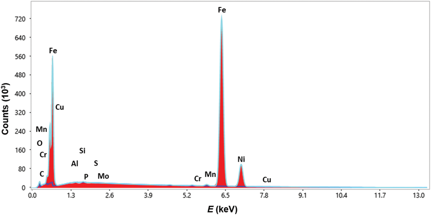
Figure 1: EDX spectrum chart of chemical composition of studied C45 steel

As for the utilized testing device, Gleeble 3800 is a universal thermal-mechanical physical simulation machine produced by Dynamic Systems Inc. (Austin, TX, USA), which can be utilized to perform complex studies of hot deformation behaviors of various materials via a variety of tests (dilatometric tests, nil strength temperature tests, tensile tests, compression tests). It is also capable of performing simulations of multi-pass forming processes. One of its mobile conversion testing units, Hydrawedge (see the photo of its testing chamber in Fig. 2a) is purposefully designed to perform hot compression tests in a wide range of deformation temperatures and strain rates, which enables to perform thorough studies of the influences of various thermomechanical conditions on the flow stress evolutions of examined materials.

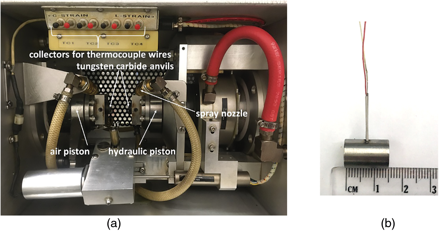
Figure 2: Gleeble 3800 Hydrawedge testing chamber (a); testing sample with welded thermocouple wires (b)

The samples for the hot compression testing were cylindrical shapes with a length of 15 mm and a diameter of 10 mm. The uniaxial compression was performed for each sample up to a true strain of −1.1. The deformation temperature and strain rate conditions were variable. Specifically, temperatures of 1173, 1273, 1373, 1473, and 1553 K were combined with strain rates of 0.1, 1, 10, and 100 s−1, which provided an experimental dataset consisting of twenty individual flow stress curves. The required deformation temperature for each testing sample was achieved via direct electrical resistance heating, and the temperature was directly measured using a pair of thermocouple wires welded on each sample in its middle length, see a photo of the prepared sample in Fig. 2b. Oxidation was prevented by keeping the testing chamber under vacuum. Before each test, the anvil-sample interface was covered with a layer of nickel-based high-temperature grease and a tantalum foil.

3  Machine Learning Regression Analysis

3.1 Preparing Experimental Dataset for Processing

The hot compression flow stress curve dataset represents a highly non-linear dependency of a single outcome, σ (true flow stress (MPa)), on three predictors—temperature, T (K), strain rate, ε˙ (s−1) and true strain, ε (-). The examined experimental dataset is, in its basic form, arranged as a two-dimensional matrix, where each row corresponds to a single T-ε˙-ε observation and the column vectors represent the individual predictors and target outcome. Since varying dimensions and ranges of the variables within the dataset can negatively influence model response and convergence speed when applying some machine learning regression techniques, the matrix columns were normalized to be dimensionless and ranging in the interval of [0,1]⊂Q (Eq. (1)) [61]:

y=x−xminxmax−xmin(1)

where x, y, xmin, and xmax are unnormalized and normalized forms of the examined matrix and minimal and maximal values of the unnormalized matrix columns, respectively. Before the strain rate predictor column was normalized, the strain rate was transformed into a logarithmic form. Although some of the above-listed ML models do not require any normalization procedure, a normalized dataset was used for all MLs to increase the reliability of subsequent comparisons of the computed data.

Given the nature of machine learning, ML regression models tend to overfit the characterized data, i.e., they return nonsensical predictions if they are not assembled with proper settings. In order to overcome this issue, ML techniques with various settings were assembled on 70% of the data of the experimentally acquired dataset (training subset), and the model’s performance was verified using the remaining 30% portion of the dataset (testing subset). The dataset split is listed in Table 2.

3.2 Essence of Applied Machine Learning Techniques

3.2.1 Artificial Neural Networks

ANNs for regression analyses are constructed to provide functional relationships between predictors and outcomes based on networks of artificial neurons arranged into layers. The structure of such a network and the nature of a neuron’s inner calculation mechanism are then influenced by the selected ANN topology, the most prominent of which are characterized below.

The standard FF-MLP model consists of an input layer, one or more hidden layers, and an output layer. The first hidden layer has a synaptic weight connection from the predictor matrix (input layer), and each subsequent layer has a connection from the previous one. The output layer then produces the FF-MLP regression model response. As for the herein presented regression, the inner calculation mechanism of the FF-MLP hidden neuron can be expressed as Eq. (2) [61,62].

aj=tanh⁡[∑i=1m(ai⋅wij)+bj](2)

where ai is the response vector (axon) of i-th neuron of a lower-level layer, aj and bj are the axon and bias of j-th neuron of a higher level layer, and wij is the synaptic weight connecting the i-th and j-th neurons. i=[1,m]⊂N and j=[1,n]⊂N, where m and n represent the number of neurons in the lower level and higher level layer, respectively. The number of neurons in the input and output layers corresponds with the number of predictors and outcomes. Since the herein presented research is only characterized by a single outcome, the final desired FF-MLP model response is a single vector returned as the linear combination of the neuron responses of the last hidden layer added to the bias b (Eq. (3)) [61,62]:

σ=∑j=1n(aj⋅wj)+b(3)

where wj is the weight connecting the j-th neuron axon of the last hidden layer with the output layer neuron, and n is the number of neurons in the last hidden layer. The number of hidden layers and neurons then represents the hyperparameters of the FF-MLP model, which have to be tuned to ensure its reliable performance. Optimization of the weights and biases from Eqs. (2) and (3) in order to minimize the network response error was, in each case, solved via the Levenberg-Marquardt optimization with the backpropagation learning algorithm and by the application of the Bayesian regularization. This optimization was performed for 20 various pseudo-randomly generated sets of initial w-b values at each combination of the examined hyperparameters.

The structure of the RBNN model and the GRNN model consists of a single input layer, an RB layer, and a single output layer. The purpose of the RB layer is to convert a non-linear regression issue into a linear form via mapping of a low-dimensional predictor feature space (R3 in the presented research) to a high-dimensional one (Rn). The inner calculation mechanism of a single RB layer neuron (RBN) can be formulated as Eq. (4) [63–65].

aj=exp⁡[−(‖Cj−P‖⋅−ln⁡(0.5)γ)2](4)

where aj and Cj are the j-th RBN axon and a corresponding neuron center, respectively; j=[1, n]⊂N, where n is the number of RBNs; ‖Cj−P‖ is the vector of Euclidean distances between the center of j-th neuron and data points of a predictor matrix, P; γ is the spread of the Gaussian function and represents a tunable hyperparameter of the RBNN and GRNN models.

For the RBNN model, its output layer’s inner calculation mechanism can be expressed similarly to the FF-MLP model, i.e., by Eq. (3). However, the GRNN model’s response is given differently, as shown in Eq. (5) [63,64].

σ=∑j=1naj⋅wj∑j=1naj(5)

The neuron centers in Eq. (4) are set to be equal to the observations of the predictor matrix (T-ε˙-ε triplets). For the RBNN model, the weights and biases of Eq. (3) are then estimated via the simple least square method, and the weights in Eq. (5) are set to be equal to the datapoints of the outcome vector (σ singletons). Based on the nature of the RBNN and GRNN models, the number of neurons in the RB layer is practically equal to the number of observations involved in the training subset. However, unlike the GRNN model, the RBNN model only employs a restricted amount of these neurons due to the collinearity phenomenon.

3.2.2 Support Vector Machine

The SVM regression model is, by its nature, similar to the RBNN method described above. The SVM approach also benefits from mapping a low-dimensional predictor space to a high-dimensional feature space, i.e., the transformation of a non-linear regression issue into a linear one. The SVM model response can be formulated via Eq. (6) [65].

σ=∑j=1n[G(SVj, P)⋅(αj−αj∗)]+b(6)

where G(SVj,P) is the j-th vector of a high-dimensional feature space, SVj is the j-th support vector, and α-values represent the corresponding Lagrange multipliers, where j=[1, n]⊂N, n is the number of predictors in the high-dimensional feature space (number of SVs). This space is represented by the Gram matrix, which is assembled based on a specific non-linear kernel function (Gaussian or polynomial). Determining the α-values and bias b is based on a linear ε-insensitive regression technique—solved via the sequential minimal optimization algorithm within the presented research. The applied regression technique brings two basic hyperparameters, which must be tuned, into the SVM model—specifically, ε-insensitive loss and box constraint. The performance of the SVM regression model is further influenced by the selection of the above kernel function and the corresponding hyperparameter (spread of the Gaussian function and polynomial order with regard to the Gaussian and polynomial kernel, respectively).

3.2.3 Decision Tree Regression

The DTR model is denominated based on its characteristic tree-like structure. The DTR model consists of nodes, which are hierarchically divided from the root node (nonterminal decision node storing the examined predictor matrix) through layers of subnodes (inner nonterminal decision nodes), to leaves (terminal nodes representing model outcomes). From the mathematical point of view, the examined predictor space is gradually divided by a sequence of decisions on a finite number of separated subspaces bound by specific intervals of examined predictors. These subspaces are further associated with specific outcome values. The DTR model response on a submitted predictor observation is thus given by the assignment to a proper subspace. For the presented research, this can be expressed by the following conditional function (Eq. (7)):

σ=rk|for T=[Tak, Tbk]∧ε˙=[ε˙ak, ε˙bk]∧ε=[εak, εbk](7)

where Tak, Tbk, ε˙ak, ε˙bk, εak, and εbk are the lower (a-subscript) and upper (b-subscript) bounds of the temperature, strain rate, and strain intervals delimiting the k-th predictor subspace. The specific k-th response (leaf) rk is returned by the DTR model when the input predictor observation falls under the corresponding k-th predictor subspace. The complexity of a decision tree, the number of predictor subspaces, and thus the number of leaves is influenced by the nature of the processed dataset, utilized learning algorithm, and model hyperparameters. As for the presented research, the interaction-curvature algorithm, for which the maximum number of decision nodes within a layer, in connection with the minimum leaf size, represent the tunable DTR model hyperparameters, was applied to determine the way the particular decision nodes are split (considering node binary partition). The resulting complexity of the assembled tree then represents a tradeoff between the response accuracy and prediction capability.

3.2.4 Gaussian Process Regression

The GPR model applies a probabilistic-based approach to predict a proper outcome response. In this research, the GPR model response can be expressed as Eq. (8) [66].

σ=H⋅β+f(8)

The GPR model consists of two main elements. The first one is given by a p×n basis matrix H, representing the projection of the original predictor space (R3 in the presented research) into a new feature space (Rn), where the space dimension n is influenced by the selection of the explicit basis function, and p is the number of observations. Then, β is the corresponding n×1 vector of basis function coefficients (one for each feature). The second element of the GPR model, f, then represents the p×1 vector of latent variables (one for each predictor observation). The vector f is considered to be distributed as a GP with a zero mean and covariance (kernel) matrix K(Ptr, Pn) (Eq. (9)) [66]:

f∼GP[0,K(Ptr,Pn)](9)

The K(Ptr, Pn) matrix determines how the response at one predictor observation is affected by responses at other observations—Ptr and Pn are predictor matrices containing training and new observations, respectively. The new observations from the testing subset are considered in the model training process. Then, the trained model is prepared to accept entirely new observations. In other words, the basic strategy behind the GPR is to get a regression model in which the residuals are modeled via GP. The K(Ptr, Pn) matrix is then assembled based on a specific kernel function—see Table 3. Considering Eq. (9), the values of the required f-vector can be acquired by incorporating the zero mean and K(Ptr, Pn) into the known multivariate Gaussian distribution model.

The performance of the GPR model is influenced by several hyperparameters: selection of the above basis function, kernel function, and the value of noise standard deviation δn. In addition, the kernel functions introduce other variables into the model—signal standard deviation δf, and characteristic length scale δl. The initial values of δn, δf, and δl parameters and the above β-values were in each case refined using the quasi-Newton optimization algorithm, and the parameters of the Automatic Relevance Determination-based kernels (GPR model) were not optimized.

3.2.5 Hyperparameter State Space

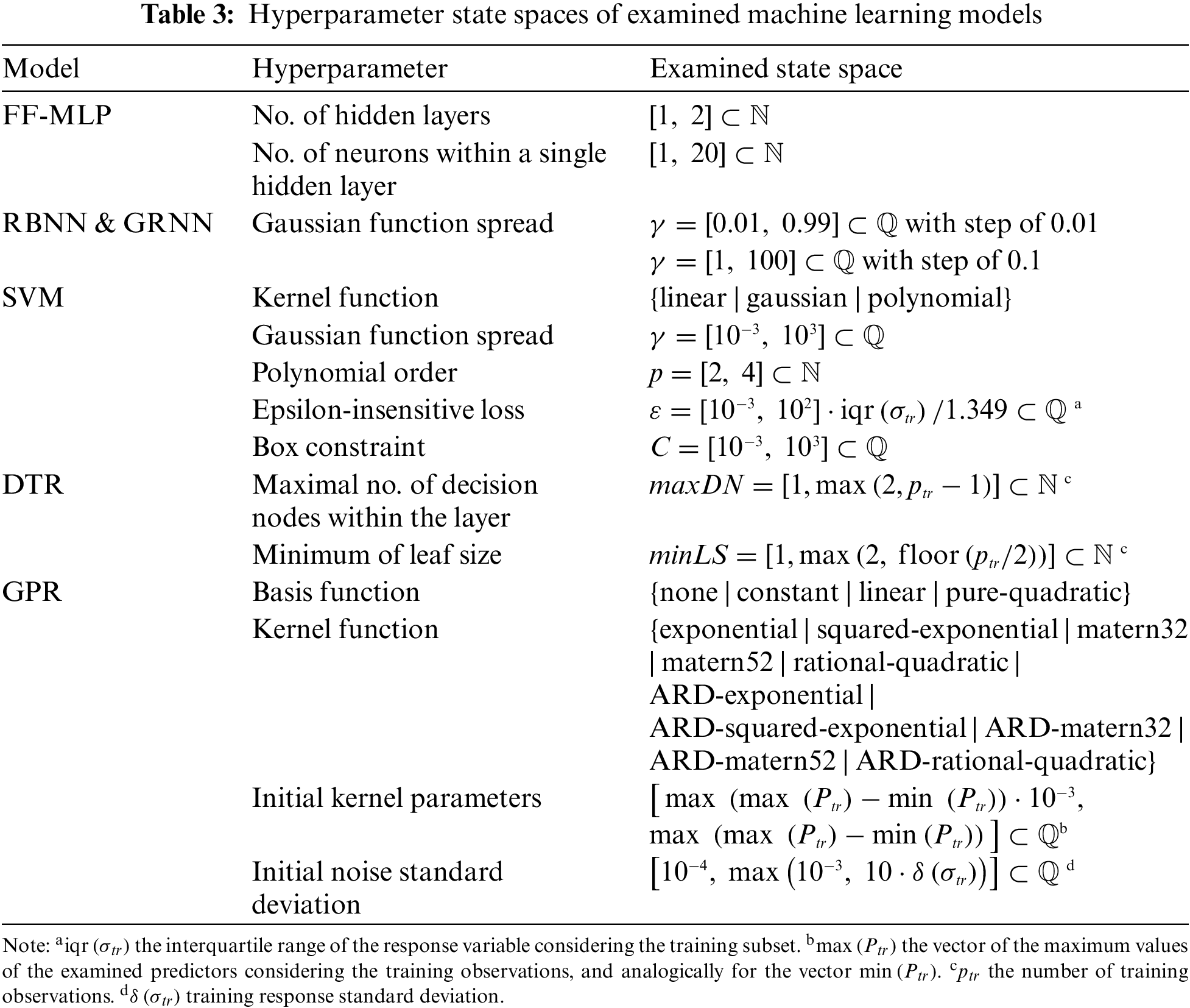
The optimal values must be estimated since the proposed machine learning models are associated with various hyperparameters. Table 3 lists their overview and the corresponding state spaces examined within the presented research. As regards the FF-MLP, RBNN, and GRNN models, the optimal hyperparameter settings were found through a trial-and-error method by testing each value of the corresponding state space. The state spaces of other models were then browsed via the Bayesian optimization algorithm.

4  Results and Discussion

Accordingly, the proposed ML-based regression models must be tuned concerning the training subset and the new observations to return a proper outcome response, i.e., to enable reliable predicting. The applied models’ reaction to new observations is evaluated using a specific testing subset, as detailed in Table 2. The optimal hyperparameters of the applied machine learning techniques, resulting from the performed tuning, are summarized in Table 4.

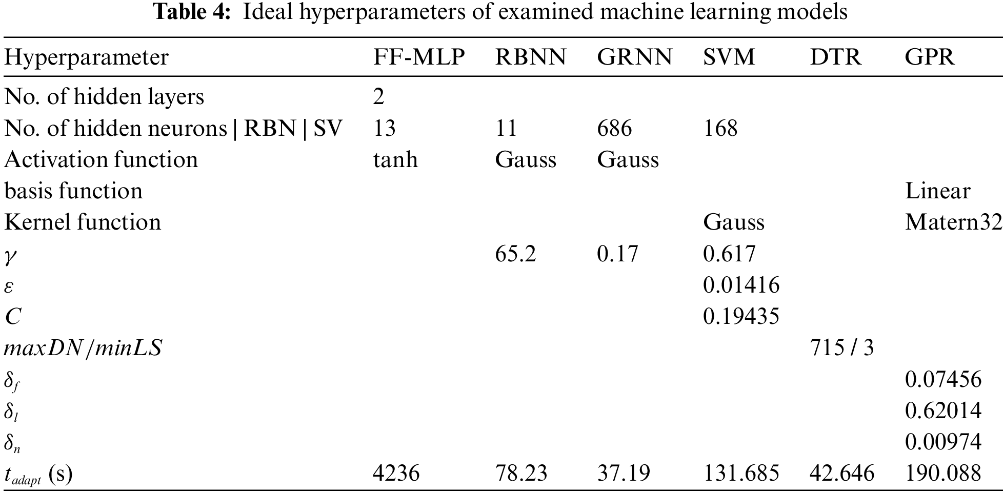
The bottom row in Table 4 summarizes adaptation runtimes for all the applied ML techniques to enable indicative comparison of the individual approaches. The most time-consuming adaptation phase (exceeds the time of an hour) is associated with the FF-MLP regression model; the other models exhibited computing times lower than 4 min, some even lower than 1 min. The fact that the FF-MLP adaptation is the most time-consuming can be directly attributed to trial-and-error searching for optimal initial weights and biases, which are repeatedly pseudo-randomly generated under each examined combination of hidden layers and hidden neurons during the computations.

The first tentative insight into the accuracy of the assembled regression models using the RMSE indicator (MPa) (Eq. (10)) is depicted in Fig. 3.

RMSE=1p⋅∑i=1pΔi2(10)

where Δi (MPa) is the difference between the i-th target and returned true flow stress response, i.e., model residuum i=[1, p]⊂N, where p is the number of data points in the training or testing (predicting) subset.

Figure 3: Comparison of root mean squared errors of examined machine learning models

Considering the returned RMSE values, the ANN-based regression models, FF-MLP, RBNN, and GRNN (especially the GRNN one), feature lower response accuracy than the other applied ML techniques. In addition, the ANN models show relatively higher differences between the training and testing subsets, implying that the reaction of the examined ANN models on a new dataset can be less reliable. Fig. 3 indicates that the SVM, DTR, and especially GPR methods offer higher fitting accuracy and predicting reliability when compared to the presented ANN models. Additional statistical indicators, namely the Mean Absolute Percentage Error (MAPE) (%) (Eq. (11)) and the coefficient of determination R2 (−) (Eq. (12)), confirm the dominant position of the GPR method, as listed in Table 5. The ANN model built on the FF-MLP architecture is very close to this GPR model’s accuracy.

MAPE=1n⋅∑i=1n|ΔiTi|⋅100(11)

R2=1−∑i=1nΔi2∑i=1n(Ti−T¯)2(12)

where Ti (MPa) and T¯ (MPa) are the i-th target true flow stress response and the mean value of target responses, respectively, for i=[1, n]⊂N, where n is the number of all data points (training and testing subset).

A box-and-whisker diagram, expressing the analysis of the returned flow stress residues simply and comprehensively, is presented in Fig. 4 to acquire a deeper insight into the accuracy of the examined models.

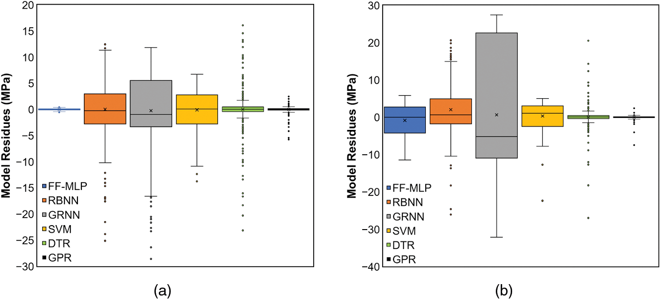
Figure 4: Box-and-whisker diagrams of returned residues: train subset (a); test subset (b)

Fig. 4 indicates that the most favorable regression response is achieved when applying the GPR model. The absolute values of residues provided by this model are for the training and testing subsets not higher than 8 MPa. The FF-MLP regression model provides the second most favorable response. The absolute residues associated with the testing subset are generally lower than 10 MPa. Fig. 4 also shows that the third model providing the most reliable response is the SVM one. As for both the training and testing subsets, the absolute residues returned from the SVM regression are, similar to the FF-MLP model, generally not higher than 10 MPa. However, the SVM residue vector contains an outlier (approx. −22 MPa) in the testing subset. Nevertheless, a detailed analysis revealed that this outlier is associated with the true strain value of 0.039, i.e., with the beginning of deformation processing (the first flow curve datapoint). From a practical point of view, a deceptive prediction for such a small strain value can be considered low in significance. Therefore, from a statistical point of view, the reliability of the SVM model can be considered comparable to that of the FF-MLP approach.

The ranges of RBNN, GRNN, and DTR model residues for the training subset are approximately from −25 to 12, −29 to 12, and −23 to 16 MPa, respectively. In other words, the scatters of these residues are prominently larger when compared to the scatters observed for the other models; similar results were also acquired for the testing subset. Regarding the DTR methodology, absolute residues higher than 10 MPa are associated with true strain values of up to 0.16, i.e., in the early deformation stage. On the other hand, for the RBNN and GRNN models, the absolute residues higher than 10 MPa are more or less homogeneously distributed through the entire strain range.

Figs. 5 and 6 further depict graphical comparisons of target flow and flow stress curves returned by the applied regression models to enhance the performed statistical analysis. Fig. 5a–d confirms the presented statistical evaluation of the ANN-based models. Neither the RBNN model nor the GRNN one can reliably follow the curve shape. This finding is consistent with the acquired large scatters of residuals presented in Fig. 4. The FF-MLP model exhibits higher reliability as it shows significant deviations only for predictions. The FF-MLP model is against the RBNN model and GRNN model more robust. The simplified architecture of the RBNN and GRNN models is not robust enough to capture the complicated nature of hot flow curves. The GRNN model, especially, whose weights are formed only by the values of the input and output variables, practically does not provide sufficient variability. Fig. 6a–d compares target flow stress curves with those returned by the other examined ML techniques. These comparisons confirm that the GPR method offers the most reliable regression performance. The training and testing subsets exhibit an incomparably higher regression fit than those acquired by the other applied models. The success of the GPR model lies in its probabilistic-based approach, where the regression model is constructed in such a way that residual values are modeled via the Gaussian process. Fig. 4 indicates that the accuracy of the SVM method is just behind the accuracy of FF-MLP. This finding is confirmed by Figs. 5 and 6; as can be seen, the SVM flow stress curve shapes deviate slightly from the target flow curve shapes but not as much as those provided by the RBNN and GRNN approaches. The SVM methodology is very close to the RBNN model. However, SVM is more robust thanks to a slightly different way of calculating the output variable, i.e., linear ε-insensitive regression technique instead of classic linear regression, which provides two other key parameters; by properly tuning them, higher accuracies can be achieved. However, as the time requirements of the RBNN and GRNN regression techniques are lower than that of the SVM approach, i.e., these techniques are fast, simple to assembly, and do not require sophisticated software, see Table 4, they can be applied if a quicker estimation (at the expense of lower reliability) is required. As also ensues from Fig. 6a–d, the DTR approach seems rather inappropriate for a reliable description of the flow stress curve. The disadvantage of the DTR method is that the assembled model divides the strain range into several subranges, and the influence of increasing strain on a flow stress change is practically omitted; see the returned groups of constant responses depicted by green points in Fig. 6a–d.

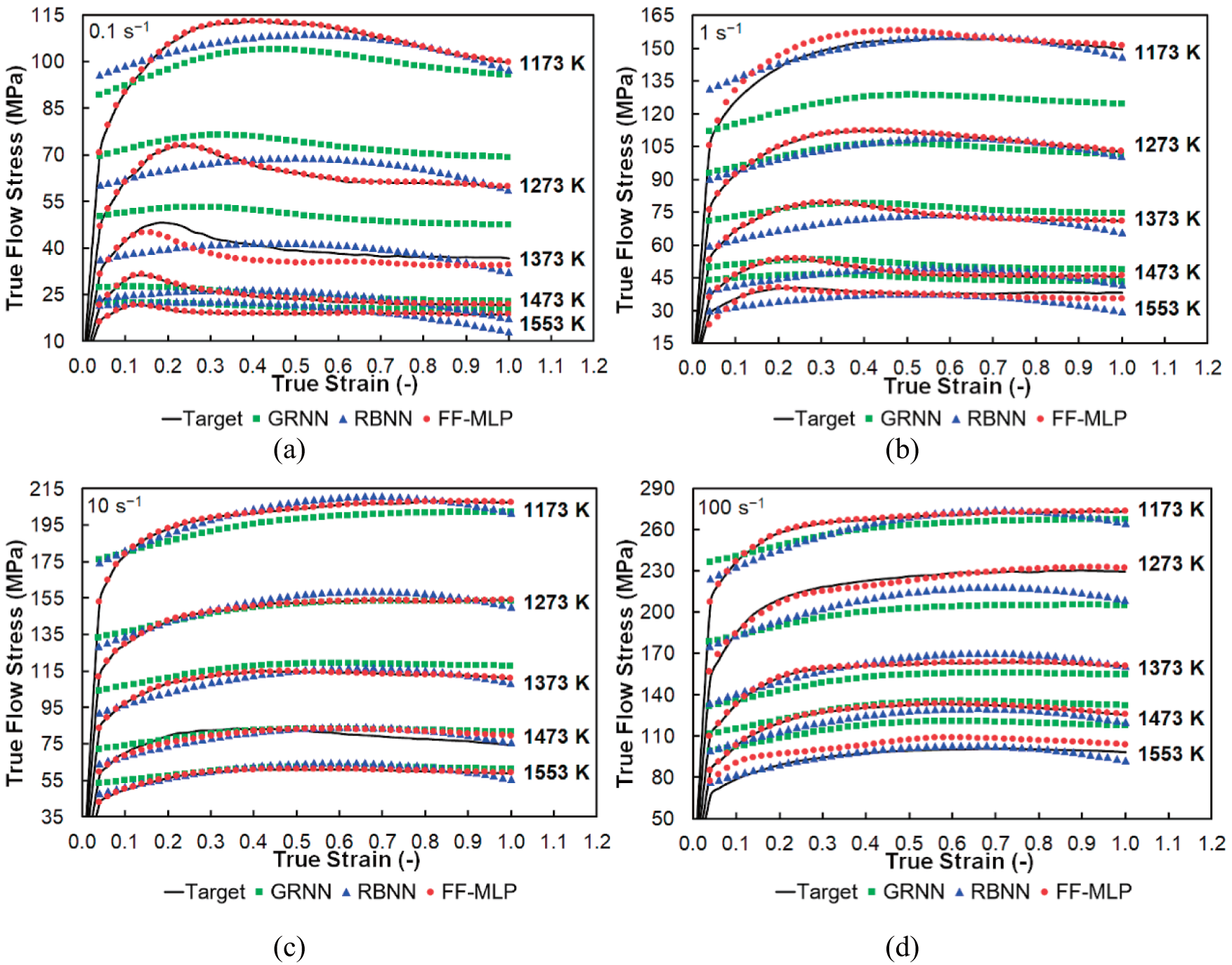
Figure 5: Comparison of target (experimental) data and data modeled via ANN-based models: strain rate of 0.1 s−1 (a); strain rate of 1 s−1 (b); strain rate of 10 s−1 (c); strain rate of 100 s−1 (d)

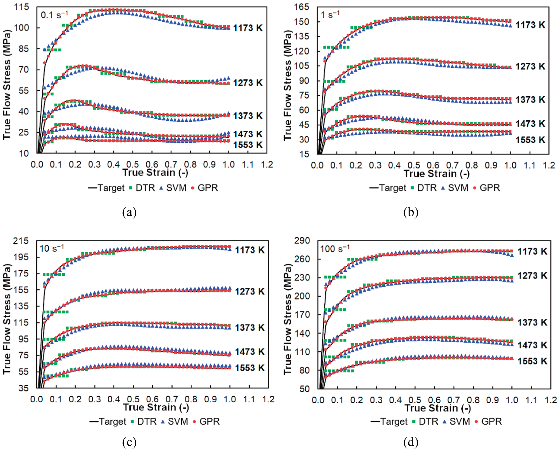
Figure 6: Comparison of target (experimental) data and data modeled via other ML-based models: strain rate of 0.1 s−1 (a); strain rate of 1 s−1 (b); strain rate of 10 s−1 (c); strain rate of 100 s−1 (d)

Table 6 further summarizes an overview of the critical characteristics of individual machine learning techniques in connection with hot flow stress response modeling.

5  Conclusions

This research presents the possibilities of various ML techniques, specifically three ANN-based methods (FF-MLP, RBNN, and GRNN), and SVM, DTR, and GPR approaches when applied to mathematically describe the evolution of flow stress for steels plastically deformed under hot conditions. Mutual comparison of the ANNs approaches shows that the FF-MLP regression offers the most favorable results; the RBNN and GRNN models featuring simpler structures failed in characterizing the experimental flow stress curves, most probably given by their shape diversity. Nevertheless, contrary to the RBNN and GRNN, the FF-MLP structure is highly non-linear and requires longer computing time. The DTR, SVM, and GPR methods also provide more reliable results than the RBNN and GRNN ones. The flow stress curve shapes calculated by the DTR method are highly inaccurate, although the predicted flow stress levels are comparable with the experimental data. Although the mathematical base of the SVM method is comparable to that of RBNN and GRNN, its higher robustness probably resulted in more reliable results as regards the flow stress curve shape diversity. The most accurate regression fit is acquired when applying the GPR method, even though this technique was not employed before to solve such a regression task. Based on the acquired results, its unique approach is practically unrivaled, and the GPR model can thus be recommended for handling tasks that deal with descriptions of hot flow stress curves. The accuracy of the GPR model is followed by the FF-MLP and SVM techniques, the application of which can also be recommended to solve such regression tasks. Nevertheless, the application of the RBNN, GRNN, and DTR models can still be considered if keeping the exact shape diversity of the modeled flow stress curves is not strictly required.

Acknowledgement: The cooperation of Jaromír Kopeček, FZU—Institute of Physics of the Czech Academy of Sciences, is greatly appreciated.

Funding Statement: The research was supported by the SP2024/089 Project by the Faculty of Materials Science and Technology, VŠB–Technical University of Ostrava.

Author Contributions: The authors confirm their contribution to the paper as follows: study conception and design: Petr Opěla, Josef Walek; data collection: Petr Opěla, Jaromír Kopeček; analysis and interpretation of results: Petr Opěla, Josef Walek; draft manuscript preparation: Petr Opěla, Josef Walek, Jaromír Kopeček. All authors reviewed the results and approved the final version of the manuscript.

Availability of Data and Materials: The data that supports the findings of this study is available from the corresponding author upon request.

Ethics Approval: Not applicable.

Conflicts of Interest: The authors declare no conflicts of interest to report regarding the present study.

References

1. Sakai T, Belyakov A, Kaibyshev R, Miura H, Jonas JJ. Dynamic and post-dynamic recrystallization under hot, cold and severe plastic deformation conditions. Prog Mater Sci. 2014;60:130–207. doi:10.1016/j.pmatsci.2013.09.002. [Google Scholar] [CrossRef]

2. Pustovoytov D, Pesin A, Tandon P. Asymmetric (hot, warm, cold, cryo) rolling of light alloys: a review. Metals. 2021;11(6):956. doi:10.3390/met11060956. [Google Scholar] [CrossRef]

3. Kunčická L, Kocich R, Lowe TC. Advances in metals and alloys for joint replacement. Prog Mater Sci. 2017;88:232–80. doi:10.1016/j.pmatsci.2017.04.002. [Google Scholar] [CrossRef]

4. Kocich R, Kunčická L, Benč M, Weiser A, Németh G. Corrosion behavior of selective laser melting-manufactured bio-applicable 316L stainless steel in ionized simulated body fluid. Int J Bioprinting. 2024;10(1):1416. doi:10.36922/ijb.1416. [Google Scholar] [CrossRef]

5. Derevyagina LS, Gordienko AI, Surikova NS, Volochaev MN. Effect of helical rolling on the bainitic microstructure and impact toughness of the low-carbon microalloyed steel. Mater Sci Eng A. 2021;816:141275. doi:10.1016/j.msea.2021.141275. [Google Scholar] [CrossRef]

6. Kocich R, Kursa M, Szurman I, Dlouhý A. The influence of imposed strain on the development of microstructure and transformation characteristics of Ni-Ti shape memory alloys. J Alloys Compd. 2011;509(6):2716–22. doi:10.1016/j.jallcom.2010.12.003. [Google Scholar] [CrossRef]

7. Volokitina I, Volokitin A, Panin E, Fedorova T, Lawrinuk D, Kolesnikov A, et al. Improvement of strength and performance properties of copper wire during severe plastic deformation and drawing process. Case Stud Constr Mater. 2023;19:e02609. doi:10.1016/j.cscm.2023.e02609. [Google Scholar] [CrossRef]

8. Galiev FF, Saikov IV, Alymov MI, Konovalikhin SV, Sachkova NV, Berbentsev VD. Composite rods by high-temperature gas extrusion of steel cartridges stuffed with reactive Ni-Al powder compacts: influence of process parameters. Intermetallics. 2021;138:107317. doi:10.1016/j.intermet.2021.107317. [Google Scholar] [CrossRef]

9. Hlaváč LM, Kocich R, Gembalová L, Jonšta P, Hlaváčová IM. AWJ cutting of copper processed by ECAP. Int J Adv Manuf Technol. 2016;86:885–94. doi:10.1007/s00170-015-8236-2. [Google Scholar] [CrossRef]

10. Kocich R, Kunčická L. Development of structure and properties in bimetallic Al/Cu sandwich composite during cumulative severe plastic deformation. J Sandw Struct Mater. 2021;23(8):4252–75. doi:10.1177/1099636221993886. [Google Scholar] [CrossRef]

11. Kocich R, Szurman I, Kursa M, Fiala J. Investigation of influence of preparation and heat treatment on deformation behaviour of the alloy NiTi after ECAE. Mater Sci Eng A. 2009;512(1–2):100–4. doi:10.1016/j.msea.2009.01.054. [Google Scholar] [CrossRef]

12. Kocich R, Greger M, Macháčková A. Finite element investigation of influence of selected factors on ECAP process. In: Metal 2010: 19th International Metallurgical and Materials Conference, 2010 May 18–20; Ostrava, Czech Republic; p. 166–71. [Google Scholar]

13. Zhang Q, Guo H, Xiao F, Gao L, Bondarev AB, Han W. Influence of anisotropy of the magnesium alloy AZ31 sheets on warm negative incremental forming. J Mater Process Technol. 2009;209(15–16):5514–20. doi:10.1016/j.jmatprotec.2009.05.012. [Google Scholar] [CrossRef]

14. Shahare HY, Dubey AK, Kumar P, Yu H, Pesin A, Pustovoytov D, et al. A comparative investigation of conventional and hammering-assisted incremental sheet forming processes for AA1050 H14 sheets. Metals. 2021;11(11):1862. doi:10.3390/met11111862. [Google Scholar] [CrossRef]

15. Macháčková A, Krátká L, Petrmichl R, Kunčická L, Kocich R. Affecting structure characteristics of rotary swaged tungsten heavy alloy via variable deformation temperature. Materials. 2019;12(24):4200. doi:10.3390/ma12244200. [Google Scholar] [PubMed] [CrossRef]

16. Wang Z, Chen J, Besnard C, Kunčická L, Kocich R, Korsunsky AM. In situ neutron diffraction investigation of texture-dependent shape memory effect in a near equiatomic NiTi alloy. Acta Mater. 2021;202:135–48. doi:10.1016/j.actamat.2020.10.049. [Google Scholar] [CrossRef]

17. Ukai S, Ohtsuka S, Kaito T, de Carlan Y, Ribis J, Malaplate J. Oxide dispersion-strengthened/ferrite-martensite steels as core materials for generation IV nuclear reactors. In: Pascal Y, editor. Structural materials for generation IV nuclear reactors. Cambridge: Woodhead Publishing; 2017. p. 357–414. doi:10.1016/B978-0-08-100906-2.00010-0. [Google Scholar] [CrossRef]

18. Perumal KE. Potential for application of special stainless steels for chemical process equipments. Adv Mater Res. 2013;794:691–6. doi:10.4028/www.scientific.net/AMR.794.691. [Google Scholar] [CrossRef]

19. Zagarin DA, Dzotsenidze TD, Kozlovskaya MA, Shkel’ AS, Rodchenkov DA, Bugaev AM, et al. Strength of a load-carrying steel frame of a mobile wheeled vehicle cabin. Metallurgist. 2020;64(5–6):476–82. doi:10.1007/s11015-020-01017-5. [Google Scholar] [CrossRef]

20. Macháčková A, Kocich R, Bojko M, Kunčická L, Polko K. Numerical and experimental investigation of flue gases heat recovery via condensing heat exchanger. Int J Heat Mass Transf. 2018;124:1321–33. doi:10.1016/j.ijheatmasstransfer.2018.04.051. [Google Scholar] [CrossRef]

21. Zach L, Kunčická L, Růžička P, Kocich R. Design, analysis and verification of a knee joint oncological prosthesis finite element model. Comput Biol Med. 2014;54:53–60. doi:10.1016/j.compbiomed.2014.08.021. [Google Scholar] [PubMed] [CrossRef]

22. Wang Z, Chen J, Kocich R, Tardif S, Dolbnya IP, Kunčická L, et al. Grain structure engineering of NiTi shape memory alloys by intensive plastic deformation. ACS Appl Mater Interfaces. 2022;14(27):31396–410. doi:10.1021/acsami.2c05939. [Google Scholar] [PubMed] [CrossRef]

23. Kunčická L, Kocich R, Németh G, Dvořák K, Pagáč M. Effect of post process shear straining on structure and mechanical properties of 316 L stainless steel manufactured via powder bed fusion. Addit Manuf. 2022;59:103128. doi:10.1016/j.addma.2022.103128. [Google Scholar] [CrossRef]

24. Kocich R, Kunčická L. Crossing the limits of electric conductivity of copper by inducing nanotwinning via extreme plastic deformation at cryogenic conditions. Mater Charact. 2024;207:113513. doi:10.1016/j.matchar.2023.113513. [Google Scholar] [CrossRef]

25. Lin YC, Chen XM. A critical review of experimental results and constitutive descriptions for metals and alloys in hot working. Mater Des. 2011;32(4):1733–59. doi:10.1016/j.matdes.2010.11.048. [Google Scholar] [CrossRef]

26. Wang Z, Zhang Y, Liogas K, Chen J, Vaughan GBM, Kocich R, et al. In situ synchrotron X-ray diffraction analysis of two-way shape memory effect in Nitinol. Mater Sci Eng A. 2023;878:145226. doi:10.1016/j.msea.2023.145226. [Google Scholar] [CrossRef]

27. Kunčická L, Kocich R. Optimizing electric conductivity of innovative Al-Cu laminated composites via thermomechanical treatment. Mater Des. 2022;215:110441. doi:10.1016/j.matdes.2022.110441. [Google Scholar] [CrossRef]

28. Wang S, Luo JR, Hou LG, Zhang JS, Zhuang LZ. Physically based constitutive analysis and microstructural evolution of AA7050 aluminum alloy during hot compression. Mater Des. 2016;107:277–89. doi:10.1016/j.matdes.2016.06.023. [Google Scholar] [CrossRef]

29. Zhang C, Zhang L, Shen W, Liu C, Xia Y, Li R. Study on constitutive modeling and processing maps for hot deformation of medium carbon Cr–Ni–Mo alloyed steel. Mater Des. 2016;90:804–14. doi:10.1016/j.matdes.2015.11.036. [Google Scholar] [CrossRef]

30. Jiang S, Wang Y, Zhang Y, Xing X, Yan B. Constitutive behavior and microstructural evolution of FeMnSiCrNi shape memory alloy subjected to compressive deformation at high temperatures. Mater Des. 2019;182:108019. doi:10.1016/j.matdes.2019.108019. [Google Scholar] [CrossRef]

31. Savaedi Z, Motallebi R, Mirzadeh H. A review of hot deformation behavior and constitutive models to predict flow stress of high-entropy alloys. J Alloy Compd. 2022;903:163964. doi:10.1016/j.jallcom.2022.163964. [Google Scholar] [CrossRef]

32. Shafaat MA, Omidvar H, Fallah B. Prediction of hot compression flow curves of Ti–6Al–4V alloy in α + β phase region. Mater Des. 2011;32(10):4689–95. doi:10.1016/j.matdes.2011.06.048. [Google Scholar] [CrossRef]

33. Shirobokov M, Trofimov S, Ovchinnikov M. Survey of machine learning techniques in spacecraft control design. Acta Astronaut. 2021;186:87–97. doi:10.1016/j.actaastro.2021.05.018. [Google Scholar] [CrossRef]

34. Biamonte J, Wittek P, Pancotti N, Rebentrost P, Wiebe N, Lloyd S. Quantum machine learning. Nature. 2017;549:195–202. doi:10.1038/nature23474. [Google Scholar] [PubMed] [CrossRef]

35. Khruschev SS, Plyusnina TY, Antal TK, Pogosyan SI, Riznichenko GY, Rubin AB. Machine learning methods for assessing photosynthetic activity: environmental monitoring applications. Biophys Rev. 2022;14:821–42. doi:10.1007/s12551-022-00982-2. [Google Scholar] [PubMed] [CrossRef]

36. Deng Y, Zhou X, Shen J, Xiao G, Hong H, Lin H, et al. New methods based on back propagation (BP) and radial basis function (RBF) artificial neural networks (ANNs) for predicting the occurrence of haloketones in tap water. Sci Total Environ. 2021;772:145534. doi:10.1016/j.scitotenv.2021.145534. [Google Scholar] [PubMed] [CrossRef]

37. Chen Y, Shen L, Li R, Xu X, Hong H, Lin H, et al. Quantification of interfacial energies associated with membrane fouling in a membrane bioreactor by using BP and GRNN artificial neural networks. J Colloid Interface Sci. 2020;565:1–10. doi:10.1016/j.jcis.2020.01.003. [Google Scholar] [PubMed] [CrossRef]

38. Ji G, Li L, Qin F, Zhu L, Li Q. Comparative study of phenomenological constitutive equations for an as-rolled M50NiL steel during hot deformation. J Alloy Compd. 2017;695:2389–99. doi:10.1016/j.jallcom.2016.11.131. [Google Scholar] [CrossRef]

39. Quan GZ, Zou ZY, Wang T, Liu B, Li JC. Modeling the hot deformation behaviors of as-extruded 7075 aluminum alloy by an artificial neural network with backpropagation algorithm. High Temp Mater Process. 2017;36(1):1–13. doi:10.1515/htmp-2015-0108. [Google Scholar] [CrossRef]

40. Wu SW, Zhou XG, Cao GM, Liu ZY, Wang GD. The improvement on constitutive modeling of Nb-Ti micro alloyed steel by using intelligent algorithms. Mater Des. 2017;116:676–85. doi:10.1016/j.matdes.2016.12.058. [Google Scholar] [CrossRef]

41. Wang YS, Linghu RK, Zhang W, Shao YC, Lan AD, Xu J. Study on deformation behavior in supercooled liquid region of a Ti-based metallic glassy matrix composite by artificial neural network. J Alloys Compd. 2020;844:155761. doi:10.1016/j.jallcom.2020.155761. [Google Scholar] [CrossRef]

42. Likas A. Probability density estimation using artificial neural networks. Comput Phys Commun. 2001;135(2):167–75. doi:10.1016/S0010-4655(00)00235-6. [Google Scholar] [CrossRef]

43. Quan GZ, Lv WQ, Mao YP, Zhang YW, Zhou J. Prediction of flow stress in a wide temperature range involving phase transformation for as-cast Ti–6Al–2Zr–1Mo–1V alloy by artificial neural network. Mater Des. 2013;50:51–61. doi:10.1016/j.matdes.2013.02.033. [Google Scholar] [CrossRef]

44. Lin YC, Liang YJ, Chen MS, Chen XM. A comparative study on phenomenon and deep belief network models for hot deformation behavior of an Al-Zn–Mg-Cu alloy. Appl Phys A: Mater Sci Process. 2017;123:68. doi:10.1007/s00339-016-0683-6. [Google Scholar] [CrossRef]

45. Lin YC, Li J, Chen MS, Liu YX, Liang YJ. A deep belief network to predict the hot deformation behavior of a Ni-based superalloy. Neural Comput Appl. 2018;29:1015–23. doi:10.1007/s00521-016-2635-7. [Google Scholar] [CrossRef]

46. Ossandón S, Reyes C, Cumsille P, Reyes CM. Neural network approach for the calculation of potential coefficients in quantum mechanics. Comput Phys Commun. 2017;214:31–8. doi:10.1016/j.cpc.2017.01.006. [Google Scholar] [CrossRef]

47. Zhong J, Sun C, Wu J, Li T, Xu Q. Study on high temperature mechanical behavior and microstructure evolution of Ni3Al-based superalloy JG4246A. J Mater Res Technol. 2020;9(3):6745–58. doi:10.1016/j.jmrt.2020.03.107. [Google Scholar] [CrossRef]

48. Setti SG, Rao RN. Artificial neural network approach for prediction of stress-strain curve of near β titanium alloy. Rare Met. 2014;33:249–57. doi:10.1007/s12598-013-0182-2. [Google Scholar] [CrossRef]

49. Tarasov DA, Buevich AG, Sergeev AP, Shichkin AV. High variation topsoil pollution forecasting in the Russian Subarctic: using artificial neural networks combined with residual kriging. Appl Geochemistry. 2018;88:188–97. doi:10.1016/j.apgeochem.2017.07.007. [Google Scholar] [CrossRef]

50. Osipov V, Nikiforov V, Zhukova N, Miloserdov D. Urban traffic flows forecasting by recurrent neural networks with spiral structures of layers. Neural Comput Appl. 2020;32:14885–97. doi:10.1007/s00521-020-04843-5. [Google Scholar] [CrossRef]

51. Willsch D, Willsch M, De Raedt H, Michielsen K. Support vector machines on the D-Wave quantum annealer. Comput Phys Commun. 2020;248:107006. doi:10.1016/j.cpc.2019.107006. [Google Scholar] [CrossRef]

52. He DG, Lin YC, Chen J, Chen DD, Huang J, Tang Y, et al. Microstructural evolution and support vector regression model for an aged Ni-based superalloy during two-stage hot forming with stepped strain rates. Mater Des. 2018;154:51–62. doi:10.1016/j.matdes.2016.09.007. [Google Scholar] [CrossRef]

53. Quan GZ, Zhang ZH, Zhang L, Liu Q. Numerical descriptions of hot flow behaviors across β transus for as-forged Ti–10V–2Fe–3Al alloy by LHS-SVR and GA-SVR and improvement in forming simulation accuracy. Appl Sci. 2016;6(8):210. doi:10.3390/app6080210. [Google Scholar] [CrossRef]

54. Song SH. A comparison study of constitutive equation, neural networks, and support vector regression for modeling hot deformation of 316L stainless steel. Materials. 2020;13(17):3766. doi:10.3390/ma13173766. [Google Scholar] [PubMed] [CrossRef]

55. Qiao L, Zhu J. Constitutive modeling of hot deformation behavior of AlCrFeNi multi-component alloy. Vacuum. 2022;201:111059. doi:10.1016/j.vacuum.2022.111059. [Google Scholar] [CrossRef]

56. Chatterjee S, Frohner N, Lechner L, Schöfbeck R, Schwarz D. Tree boosting for learning EFT parameters. Comput Phys Commun. 2022;277:108385. doi:10.1016/j.cpc.2022.108385. [Google Scholar] [CrossRef]

57. Lim SS, Lee HJ, Song SH. Flow stress of Ti-6Al-4V during hot deformation: decision tree modeling. Metals. 2020;10(6):739. doi:10.3390/met10060739. [Google Scholar] [CrossRef]

58. Chaudry UM, Jaafreh R, Malik A, Jun TS, Hamad K, Abuhmed T. A comparative study of strain rate constitutive and machine learning models for flow behavior of AZ31-0.5 Ca Mg alloy during hot deformation. Mathematics. 2022;10(5):766. doi:10.3390/math10050766. [Google Scholar] [CrossRef]

59. Ren O, Boussaidi MA, Voytsekhovsky D, Ihara M, Manzhos S. Random sampling high dimensional model representation Gaussian process regression (RS-HDMR-GPR) for representing multidimensional functions with machine-learned lower-dimensional terms allowing insight with a general method. Comput Phys Commun. 2022;271:108220. doi:10.1016/j.cpc.2021.108220. [Google Scholar] [CrossRef]

60. Guirguis D, Hamza K, Aly M, Hegazi H, Saitou K. Multi-objective topology optimization of multi-component continuum structures via a Kriging-interpolated level set approach. Struct Multidisc Optim. 2015;51:733–48. doi:10.1007/s00158-014-1154-3. [Google Scholar] [CrossRef]

61. Beale MH, Hagan MT, Demuth HB. Neural Network ToolboxTM 7: User’s guide. Natick: The MathWorks Inc.; 2010. [Google Scholar]

62. Opěla P, Schindler I, Kawulok P, Kawulok R, Rusz S, Sauer M. Shallow and deep learning of an artificial neural network model describing a hot flow stress evolution: a comparative study. Mater Des. 2022;220:110880. doi:10.1016/j.matdes.2022.110880. [Google Scholar] [CrossRef]

63. Opěla P, Schindler I, Kawulok P, Kawulok R, Rusz S, Navrátil H. On various multilayer perceptron and radial basis function based artificial neural networks in the process of a hot flow curve description. J Mater Res Technol. 2021;14:1837–47. doi:10.1016/j.jmrt.2021.07.100. [Google Scholar] [CrossRef]

64. Qiao L, Wang Z, Zhu J. Application of improved GRNN model to predict interlamellar spacing and mechanical properties of hypereutectoid steel. Mater Sci Eng A. 2020;792(1):139845. doi:10.1016/j.msea.2020.139845. [Google Scholar] [CrossRef]

65. Tan XH, Bi WH, Hou XL, Wang W. Reliability analysis using radial basis function networks and support vector machines. Comput Geotech. 2011;38(2):178–86. doi:10.1016/j.compgeo.2010.11.002. [Google Scholar] [CrossRef]

66. MathWorks Help Center (© 1994–2024 The MathWorks, Inc.). Documentation. Gaussian process regression models. Available from: https://www.mathworks.com/help/stats/gaussian-process-regression-models.html. [Accessed 2023]. [Google Scholar]