
 Submit a Paper
 Propose a Special lssue
 Open Access
ARTICLE

Multi-Step Clustering of Smart Meters Time Series: Application to Demand Flexibility Characterization of SME Customers
1 Department of Computer Sciences and Automatic Control, Universidad Nacional de Educación a Distancia (UNED), Madrid, 28040, Spain
2 Iberdrola Innovation Middle East, Doha, 210177, Qatar
* Corresponding Author: Santiago Bañales. Email:
(This article belongs to the Special Issue: Advanced Artificial Intelligence and Machine Learning Methods Applied to Energy Systems)
Computer Modeling in Engineering & Sciences 2025, 142(1), 869-907. https://doi.org/10.32604/cmes.2024.054946
Received 12 June 2024; Accepted 25 October 2024; Issue published 17 December 2024
 View Full Text
 Download PDF
Abstract
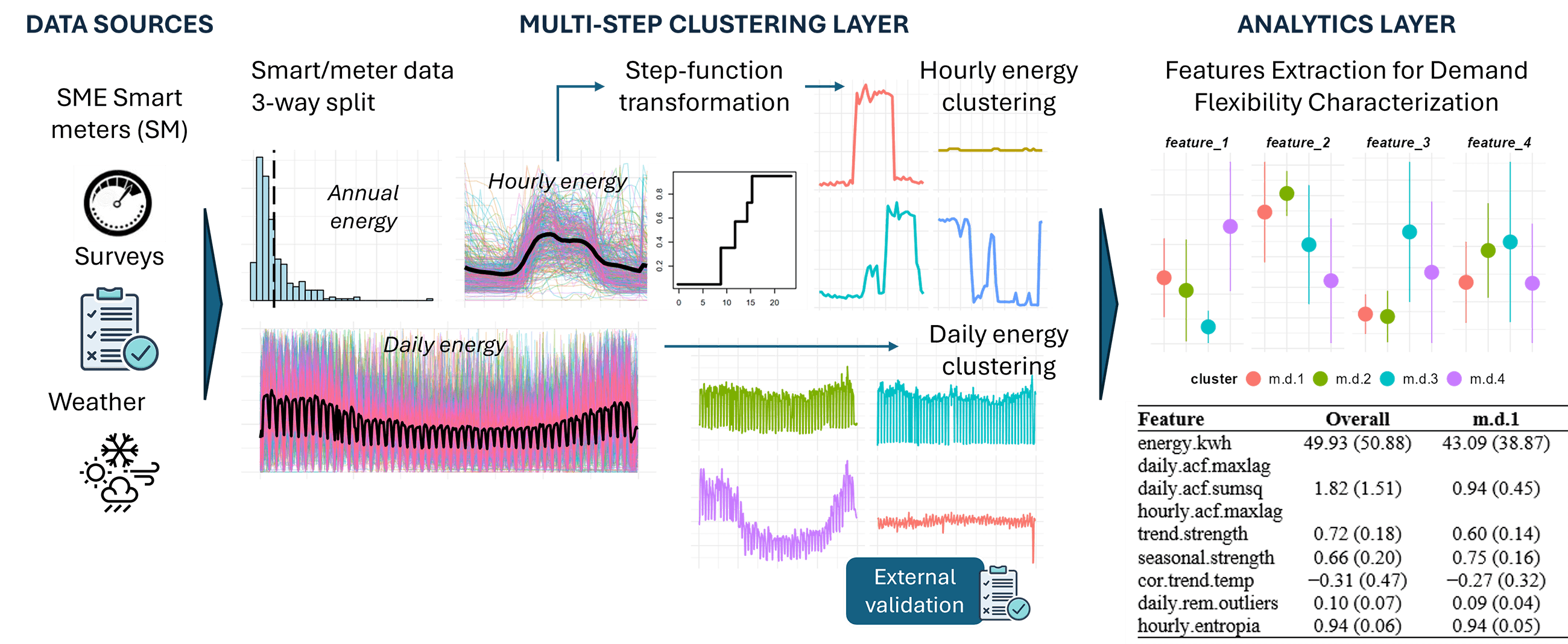
Customer segmentation according to load-shape profiles using smart meter data is an increasingly important application to vital the planning and operation of energy systems and to enable citizens’ participation in the energy transition. This study proposes an innovative multi-step clustering procedure to segment customers based on load-shape patterns at the daily and intra-daily time horizons. Smart meter data is split between daily and hourly normalized time series to assess monthly, weekly, daily, and hourly seasonality patterns separately. The dimensionality reduction implicit in the splitting allows a direct approach to clustering raw daily energy time series data. The intraday clustering procedure sequentially identifies representative hourly day-unit profiles for each customer and the entire population. For the first time, a step function approach is applied to reduce time series dimensionality. Customer attributes embedded in surveys are employed to build external clustering validation metrics using Cramer’s V correlation factors and to identify statistically significant determinants of load-shape in energy usage. In addition, a time series features engineering approach is used to extract 16 relevant demand flexibility indicators that characterize customers and corresponding clusters along four different axes: available Energy (E), Temporal patterns (T), Consistency (C), and Variability (V). The methodology is implemented on a real-world electricity consumption dataset of 325 Small and Medium-sized Enterprise (SME) customers, identifying 4 daily and 6 hourly easy-to-interpret, well-defined clusters. The application of the methodology includes selecting key parameters via grid search and a thorough comparison of clustering distances and methods to ensure the robustness of the results. Further research can test the scalability of the methodology to larger datasets from various customer segments (households and large commercial) and locations with different weather and socioeconomic conditions.Graphic Abstract
Keywords
Nomenclature
| ACF | Autocorrelation Correlation Factors |
| BAX | Binary Aggregate approXimation |
| CER | Irish Commission for Energy Regulation |
| COP26 | Conference of the Parties (United Nations Framework Convention on Climate Change (UNFCCC) hosted in the UK in 2021 |
| DER | Distributed Energy Resources |
| DR | Demand Response |
| DSM | Demand Side Management |
| DTW | Dynamic Time Warping |
| ELC | Electrical Load Clustering |
| EV | Electrical Vehicles |
| HC | Hierarchical Clustering |
| LSD | Load Shape Dictionary |
| PAA | Piecewise Aggregate Approximation |
| PAM | Partition Around Medoids |
| PCA | Principal Component Analysis |
| SME | Small and Medium Enterprises |
| STL | Seasonal and Trend decomposition using Loess |
| Notation | |
| Number of customers in a dataset | |
| Customer index | |
| Number of days with data | |
| Day index | |
| Number of data points per day | |
| Hour index | |
| Number of attributes in a customer survey | |
| Number of attributes after binarization | |
| Vector of attribute values for customer | |
| Value of attribute | |
| Average use of energy during the period for each customer | |
| Normalized daily energy time series for customer | |
| Normalized daily energy for customer | |
| Daily shape-load time series for customer | |
| Vector of daily load-shape for customer | |
| Component of | |
| Step function transformed daily shape-load time series for customer | |
| Vector of step function daily load-shape for customer | |
| Step function component of | |
| Daily Clustering: Identification of Daily Load-Shape Representatives Per Customer | |
| Input to the clustering procedure | |
| Number of daily load-shape customer clusters | |
| Set of daily load-shape customer cluster centers | |
| Center of cluster | |
| Vector of cluster members for cluster | |
| Cluster labels categorical vector, | |
| Hourly Clustering #1: Identification of Day-Unit Representatives Per Customer | |
| Input to the clustering procedure | |
| Number of clusters (i.e., representatives) per customer | |
| Set of clustering centers for customer | |
| Center of customer | |
| Set of cluster members for customer | |
| Vector of cluster labels vector for customer | |
| Hourly Clustering #2: Selection of Standard Day-Unit Hourly Profiles | |
| Input to the clustering procedure | |
| Number of standard daily load-shape clusters (i.e., representatives) | |
| Set of clustering standard daily load-shape centers | |
| Center of cluster | |
| Vector of cluster label for customer | |
| Vector of cluster label for customer | |
| Hourly Clustering #3; Customers’ Hourly Load-Shape Clustering | |
| Input to the clustering procedure | |
| Input to the clustering procedure | |
| Number of load-shape customer clusters (segments) | |
| Set of load-shape customer cluster centers | |
| Center of cluster | |
| Vector of cluster members for cluster | |
| Cluster labels categorical vector, | |
Fulfilling the intent of signatory countries of COP26, the 2021 United Nations Climate Conference pact to keep global temperature increase below 1.5°C by 2050 will require a drastic electrification of energy demand, a massive investment in renewable and storage technologies and a significant improvement in energy efficiency indicators [1]. The customer-citizen is called upon to play an instrumental role in this unprecedented transformation of our energy system, with optimization of energy use and digital citizen engagement being two of the critical interrelated information systems themes that enable Climate-Intelligent Cities [2]. New business models arise from the progressive adoption of Distributed Energy Resources (DER), Electrical Vehicles (EVs), smart meters, and business platforms, transforming the traditional passive energy user into a “prosumer” capable of generating, trading, and consuming electricity in an optimized way as a single agent [3], as part of energy communities [4,5] and/or aggregation agents [6]. The digitalization of the energy system is a crucial element to catalyze and facilitate the effective participation of the customer-citizen in such a radical transformation of our energy system [7]. Smart meters play a crucial role as an interface between the customer, enabling the adoption of new technologies (renewable DERs, energy storage, EVs, and energy management platforms) and the overall energy system [8]. Although the first generation of smart meter systems focused on relatively simple functionalities, such as improving the billing cycle, they are now an essential tool that enables a large set of real-time services, such as awareness, market participation, scheduling and control, and network services [9]. Customer participation in these markets and services is not an easy task. Data-driven platforms owned and managed by utilities, retailers, and/or energy services companies can be employed to design value propositions, segment customers, and deliver advanced automated energy services such as effective pricing and tariff design [10], distributed generation of solar energy [11], energy efficiency and conservation in buildings [12] or the provision of demand response and flexibility services [13].
Clustering customers according to similar energy usage patterns is one of the most significant applications of smart meters time-series analysis [14]. Following the massive deployment of smart meters in the last two decades, Electric Load Clustering (ELC) has been widely utilized to design personalized pricing schemes, select customers for energy efficiency, demand flexibility programs, and improve the computational efficiency of load forecasting [15,16]. The provision of demand flexibility services, the ability of electrical demand to adapt consumption patterns in reaction to signals from a system operator, is becoming increasingly important in the context of a massive integration of intermittent and fluctuating renewable generation into the energy systems as one of the strategies to balance supply and demand in different time horizons [17–19].
This paper aims to define and test a computationally efficient multi-step clustering methodology for segmenting customers based on their potential to provide demand flexibility services. There are four critical contributions to the approach. First, a smart meters’ time series split between daily and hourly normalized load profiles is introduced to allow a differentiated assessment of seasonal (month-by-month), daily (day vs. night), and intraday (hour-by-hour) effects of demand flexibility. Second, a 3-step sequential clustering approach with complexity reduction is introduced to segment the intraday hourly profiles considering the changing patterns of electrical load shape over days, weeks, and months. Third, customer metadata obtained from surveys is employed to extract customers’ and premises’ attributes and compute external validation clustering metrics. Fourth, time series decomposition techniques are utilized to construct a coherent set of data-driven demand flexibility metrics that characterize each customer and cluster regarding demand flexibility potential. This methodology is applied to a dataset of SME customers, providing deep insights into the energy profile of this critical customer segment. SMEs are seldom analyzed in the available energy profiling literature, even though SMEs represent a significant share of final energy use, estimated at ~13% worldwide [20] and between 9% and 18% in different members of the European Union [21], and have great potential for energy efficiency and conservation [22].
The rest of the paper is structured as follows. Section 2 provides a succinct literature review, identifying critical gaps related to clustering applications for demand flexibility. Section 3 presents the methodology and the theoretical tools and highlights the main methodological contributions. Section 4 describes the dataset employed to test the methodology and shows and discusses the results applied to this dataset. Finally, Section 5 presents the main conclusions and determines potential topics for further research.
Since the start of global smart meters’ deployment in the early 2000s, much research has focused on applying time series clustering techniques to profile high-frequency energy use data. Load profiling using smart meter data has been used for several applications, such as load forecasting [23], theft detection [24], and the design of Demand Side Management (DSM) or Demand Response (DR) programs [25]. Three key topics emerge from research on time series clustering: dimensionality reduction, clustering techniques, and validity indicators [26,27]. The most widely used approach to reduce the dimensionality of time series is based on transforming time series into static data by extracting ad-hoc features, such as aggregation of energy use data over user-defined periods, extraction of daily and/or seasonal averages, maximum and/or minimum values, load factor ratios or different measures of contribution to the peak of the system [28]. For instance, in [29], the study defines features based on three categories: the raw time series data, the peak at different parts of the day, and statistical descriptors such as mean, standard deviation, and percentiles. After identifying an optimal number of clusters by comparing different methods applied to this set of features, the study employs the customer’s features as predictors in a classifier to assign a probability of membership to a given cluster. Raw data clustering using Dynamic Time Warping (DTW) distance, without the use of complexity reduction techniques, has also been applied to smart meter datasets, but their wide applications are constrained by the computational needs of such an approach [30,31]. The most widely used technique for clustering smart meters time series data is k-center approaches, including k-means and k-medoids [16,32] and their fuzzy version [33]. Internal clustering validation indicators, such as the Mean Adequacy index, Cluster Dispersion index, Davies-Bouldin index, and the Average Silhouette index, are often utilized to evaluate the quality of clustering results and the optimal number of clusters [16,32], being the use of external validation indexes seldom applied [34].
This feature-based approach to complexity reduction has two main drawbacks. First, selecting representative metrics is somewhat arbitrary and subject to expert-based knowledge. Second, adopting an averaging representation method can neglect critical aspects related to the multiple consumption patterns that a customer may have during the temporal period covered by the smart meter’s time series [35]. A more structured approach is to apply formal data representation techniques, encompassing data-adaptive, non-data-adaptive, and model-based approaches [36]. Several of these formal data representation techniques have been applied to smart meter datasets, such as clipping [28,37], Fourier transforms [38], Principal Component Analysis (PCA) [39], quantile auto-covariances [40], or time series Autocorrelation Correlation Factors (ACF) [41]. Deep learning times series clustering techniques have also been applied to infer hidden non-linear features to better represent the electrical load pattern. These techniques have been found to perform better than classical techniques on high-dimensionality smart meter data with the advantage of automatic selection of representative features [42]. Eskandarnia et al. [43] used an autoencoder framework representing data as a hierarchy within deep network layers, allowing for dimensionality reduction and highly nonlinear decision separation between clusters at the autoencoder bottleneck level. Xiao et al. [44] deployed a fully connected dense layer architecture to cluster customers based on the potential for participation in Demand Response (DR) programs.
Crossing smart meter data with other information sources, such as weather and customer attributes, has also been widely employed to improve clustering quality and provide better characterization. Sandoval Guzmán et al. [45] proposed a dimensionality reduction approach based on matrix-tensor decomposition applied to a hybrid set of internal (smart meters) and external (weather) variables. Socio-economic information was used as a feature of a deep learning model in [46] to predict the likelihood of a household’s membership to a given load pattern cluster. A similar approach is applied in [47], where cluster membership was analyzed using classification and variable selection methods on a set of 26 building characteristics. Vahedi et al. [48] developed a distributed auto-clustering approach for load profile segmentation and temperature-based categories defined as group days with similar temperatures.
Another central aspect of smart meter time series clustering is considering the evolution of load profile patterns over time. Understanding seasonality and trend patterns is vital in determining the usefulness of load profile clustering in tariff design and DSM applications. Simplistic approaches to dimensionality reduction based on average feature values over time fail to capture this essential aspect. Several approaches have been proposed in the literature to model the time variation of load patterns. Li et al. [49] designed a bi-level clustering method to group customers by shape similarity, and a one-step Markov chain was employed to model the dynamics of load profiles over time. The co-clustering approach used in [47] allows the days of observation and the seasonality embedded in the temporal data to be considered in the clustering procedure.
A different approach to capturing load patterns over time involves identifying typical daily demand archetypes, also called standard profiles or representative load shapes and analyzing their temporal evolution for each customer and cluster. Eight typical demand archetypes are identified in the literature [50], and the structure of their temporal evolution is analyzed for 13,000 households in the UK over three years. The analysis identifies the effects on trends and seasonality of external attributes such as temperature conditions, calendar effects (weekends and vacation periods), and exceptional events such as the COVID-19 pandemic. Using a 3-step k-means clustering, Zhan et al. [51] identified six typical profiles in 81 buildings in Singapore and characterized the evolution of these profiles across a temporal matrix of days of the week (Monday to Sunday) and week of the year. A two-step clustering methodology was followed in the literature [31] to create a Load Shape Dictionary (LSD) that identifies representatives at both the local (customer) and global (population) levels. Therefore, the 2-step and LSD approach provides a better understanding of load shape patterns and facilitates the scalability of larger datasets. Similarly, Mets et al. [52] employed a two-stage clustering approach to identify typical daily usage patterns for individuals and coherent groups of individuals in a second stage. Fang et al. [53] encoded each daily load curve into a three-element alphabet by implementing a 2-step procedure that includes a dimensionality reduction based on the similarity of adjacent timestamp loads and a binary aggregate approximation (BAX). Multi-step clustering of smart meters data has been shown to provide additional benefits such as better capture of building operational characteristics [51], better preservation of the distribution and shape patterns present in the data [54], and a more accurate representation of the load shape temporal patterns and peak demands trough cluster merging in steps [55].
Multi-step clustering is particularly suitable for DSM applications. In addition to the advantages of multi-step clustering discussed in the previous paragraph, multi-step clustering based on local and global daily load profiles allows the characterization of load-shape patterns, including seasonality trends over different time horizons, at both the customer and group of customers levels. Distinguishing energy use patterns over time is key for selecting customers for DSM programs and customizing price-based schemas for demand flexibility. Therefore, building on the literature [28], this study proposes a multi-step time series clustering approach based on the identification of typical daily load profiles at the customer and population level, introducing several new contributions to the existing literature:
• A split and normalization of the data into daily and intraday time series makes it possible to analyze the effects of seasonality in different periods. Although the splitting procedure does not imply a loss of information, it reduces complexity by allowing a direct approach to clustering raw data from the daily energy times series data.
• Regarding normalized intraday hourly times series data, dimensionality reduction is achieved by applying a step-function transformation procedure, allowing a flexible identification per customer and cluster of periods of similar energy use during the typical day.
• Local and global intraday standard hourly load profiles are identified using a fully automated 2-step clustering approach with stopping criteria to detect the optimal number of clusters based on the decreasing reduction of intra-cluster distance.
• Although most of the literature proposes a 2-stage clustering approach to identify typical daily load profiles, this study introduces a third clustering step to group customers based on the similarity of temporal patterns of the daily load profiles. Accordingly, a new metric is introduced based on a distance-matrix computation.
• External clustering validation is performed using customer attributes embedded in surveys relevant to demand flexibility, such as the schedule of operations or thermostatic loads (cooling and heating).
• New data-driven demand flexibility features are extracted from a structured time series analysis to characterize each customer and each cluster from a demand flexibility perspective along four axes: volume, temporal baseline, consistency, and variability. This feature extraction is performed at different clustering levels, highlighting the importance of a multi-step approach to better characterize demand flexibility potential.
• Clusters are rigorously characterized using statistical tests by crossing smart meter data with building attributes and weather information.
• Extensive comparisons are made between dissimilarity metrics, clustering methods, and complexity reduction techniques to demonstrate the robustness of the proposed methodology.
• To the best of the authors’ knowledge, it is the first time that a dataset of SME customers has been employed to solve the problem of clustering based on load shape patterns.
Fig. 1 summarizes the interrelationship between the four blocks of the proposed methodology: (1) smart meter’s time series split into three components; (2) customers’ clustering according to daily energy load-shape patterns; (3) customer’s clustering based on intraday hourly load-shape patterns; (4) extraction of demand flexibility metrics from time series features and characterization of daily energy load-shape patterns. The methodology has been implemented using R language [56] running in a virtual machine cluster of 30 GB of RAM and 16 cores.
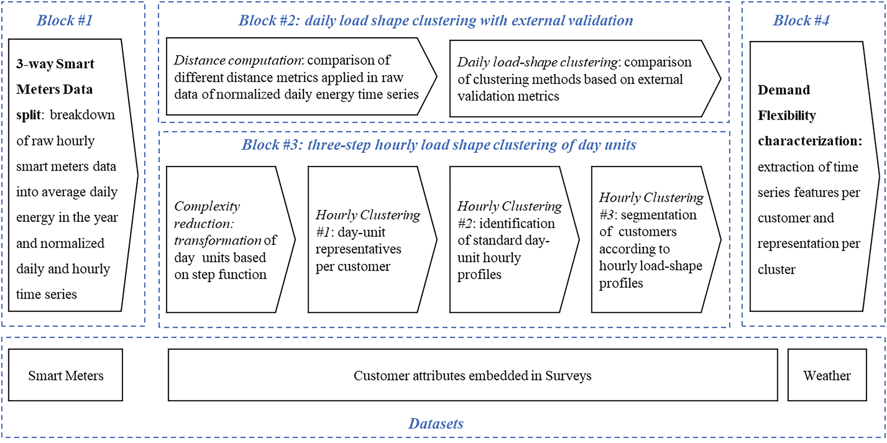
Figure 1: Methodology blocks
3.1 Block 1: Three-Way Split of Smart Meters Time Series
The methodology of this paper is based on two principles: the consideration of the calendar day as the critical time unit in time series analysis and the differentiated assessment between daily and hourly load-shape patterns. These principles are implemented by first extracting the average use of energy
3.2 Block 2: Clustering of Daily Customer’s Load Shape with External Validation
The normalized daily energy time series
Cramer’s V correlation coefficient between clusters’ vectors and selected operational and equipment customer attributes is used as an external validation metric [57]. Cramer’s V correlation coefficient between the two categorical vectors is calculated using the expression
The application of the daily load shape clustering procedure results in the identification of a set
3.3 Block 3: A Three-Step Hourly Load Shape Clustering of Day-Units with Complexity Reduction
This study implements a novel approach to normalize hourly load-shape time series in two phases: (1) complexity reduction using, for the first time to the authors’ knowledge, a step function approach and (2) a 3-step clustering pipeline based on the sequential extraction of the hourly load-shape day-unit representatives using an automated stop criterion.
3.3.1 Complexity Reduction of Day-Units via Step Function Transformation
Complexity reduction is achieved in two steps. First, the normalized shape
3.3.2 Hourly Clustering #1: Day-Unit Representatives per Customer
The first clustering step consists of identifying day-unit representatives for the hourly load-shape vector,
where
Hourly Clustering #1 represents a significant reduction in data complexity, as each customer is now represented only by
3.3.3 Hourly Clustering #2: Identification of Standard Day-Unit Hourly Profiles
In the second step of clustering, standard day-unit load-shape profiles are selected for the entire customer population at the union. Each customer day-unit representative found in the first clustering step
The Hourly Clustering #2 results in the identification of a set
The results obtained by following this approach for complexity reduction and the automatic stop criterion for Hourly Clustering #1 and #2 depending on the choice of the critical parameters of the number of steps
3.3.4 Hourly Clustering #3: Customers’ Segmentation according to Hourly Load-Shape Patterns
After Hourly Clustering #2, each customer is represented by two-time series equal to the number of days: a numerical time series containing the normalized daily energy and a categorical time series containing the s cluster labels of the standard daily profiles. The goal of Hourly Clustering #3 is to segment the population based on a measure of the total distance between its load-shape representatives over the total number of days. Since each customer’s hourly load shape is represented by one of the standard load profiles assigned in Hourly Clustering #2, a measure of the total distance between two customers will be the sum of the distance between each corresponding standard load profile for each day over the number of days with data. Hence, Table 1 shows a hypothetical example where only two standard load-shape profiles result from Hourly Clustering #2, i.e., {A, B}, representing the standard load profile corresponding to two customers, X and Y, for each of the days with data. A 2 × 2 symmetric dissimilarity matrix is defined for the standard load profiles, where the diagonal values are

This procedure was implemented using a computationally efficient matrix-based approach. The load-shape time series of each customer
where
Customer segments for Hourly Clustering #3 are computed by comparing two clustering methods, k-medoids and Hierarchical Clustering, with the ad-hoc distance matrix described above as a measure of dissimilarity. The comparison between the two methods and selecting the optimal number of clusters is performed using Cramer’s V correlation between the clustering labels vector and the operational and equipment attributes as external validation.
3.4 Block 4: Definition of Demand Flexibility Metrics via Time Series Feature Engineering
There is a lack of consensus on a standard definition of metrics that characterize the demand flexibility of buildings [61,62]. Villar et al. [18] identified the following demand flexibility attributes: power modulation amount, Duration, Rate of change, Response time, Location (transmission or distribution grid node), Delivery time, Time availability periods, Predictability, and Controllability. Luo et al. [62] differentiated between power and energy availability, emphasized the role of temporality, i.e., the evolution of load-shape over time, and added economic-related attributes to characterize demand flexibility. Flexibility Up and Down, i.e., the differentiation between the flexibility to increase or decrease power consumption and the quantification of ramp-up and rebound effects, is also critical for detailed modeling of demand flexibility at the specific equipment level [61]. Three categories of attributes are considered essential in the literature [35] to characterize the demand response: the consideration of multiple consumption patterns over time, the consistency of consumption patterns, and peak contribution metrics. Finally, the characterization of variability, in the form of (for example) entropy measurements, is essential to estimate the attractiveness of a given customer to different demand response programs: the customer with intrinsic variability would be more suitable for demand response price-based programs, while customers with lower variability will be more suitable for incentive-based programs due to the greater predictability of their consumption [63]. Table 2 lists the 16 data-driven metrics proposed in this paper to characterize demand flexibility. These metrics are derived from the smart meter’s time series features related to four different categories: Energy (E), Temporal patterns (T), Consistency (C), and Variability (V).
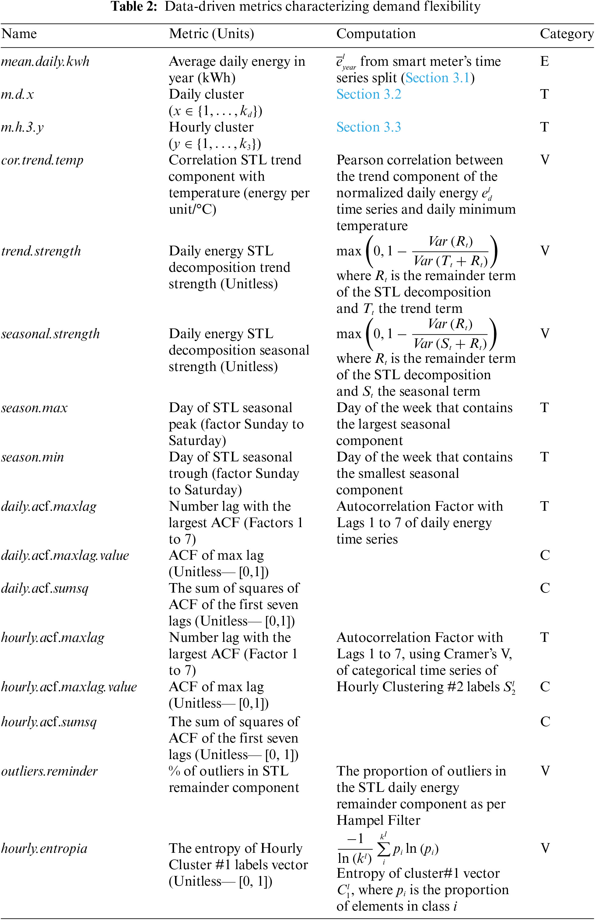
Energy (E) is the volume of energy potentially available for demand flexibility purposes, represented by the average daily energy use during the analysis period. Temporal patterns (T) are the underlying temporal structure of energy use, characterized by trend and seasonality patterns. Seasonal and Trend decomposition using Loess (STL) [64] is used on the daily time series
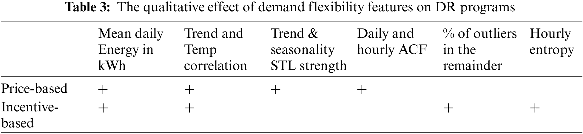
This set of features is employed to characterize the potential for demand flexibility for each customer, individually and as part of a given daily or hourly cluster, and to characterize their suitability for different DR programs. Table 3 lists a qualitative assessment of the impact of Energy, Consistency, and Variability on the suitability of different customers or sets of customers for price-based or incentive-based DR programs. Higher mean energy and greater correlation with temperature are positive indicators for any DR program. Customers with stronger trends, seasonality components, and larger ACF factors will be better suited for this category of programs to the extent that predictability is a determinant of success in price-based programs. Similarly, customers with a larger unexplained variation in daily energy and hourly patterns will be better suited for incentive-based programs. Temporal patterns will help select customers when specific timeframes for demand flexibility are targeted, such as customers with higher energy use on weekends, during the evening, or during the summer period.
4.1 Block #1: Description of the Dataset and Energy Time Series Split
The methodology was applied to the smart meter dataset from the Irish Commission for Energy Regulation (CER) publicly available smart metering trial [67]. This dataset has been widely used in the literature due to the high quality of the data and the available characterization of customers through surveys. Instead of focusing, like most previous research, on residential customers, the methodology is applied to the SME dataset for the first time, to the authors’ knowledge. A significant advantage of using the Irish CER dataset is the ease of replicability.
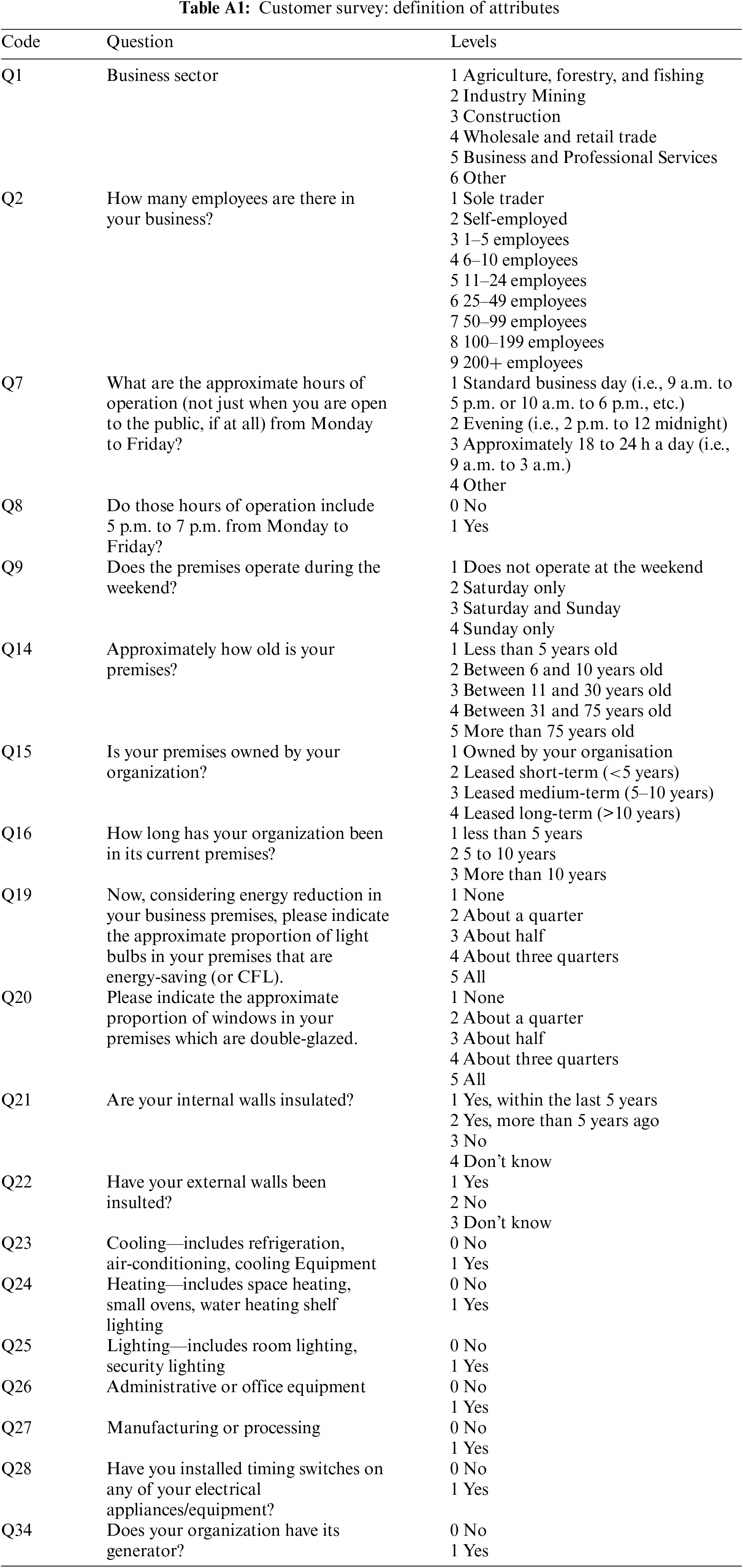
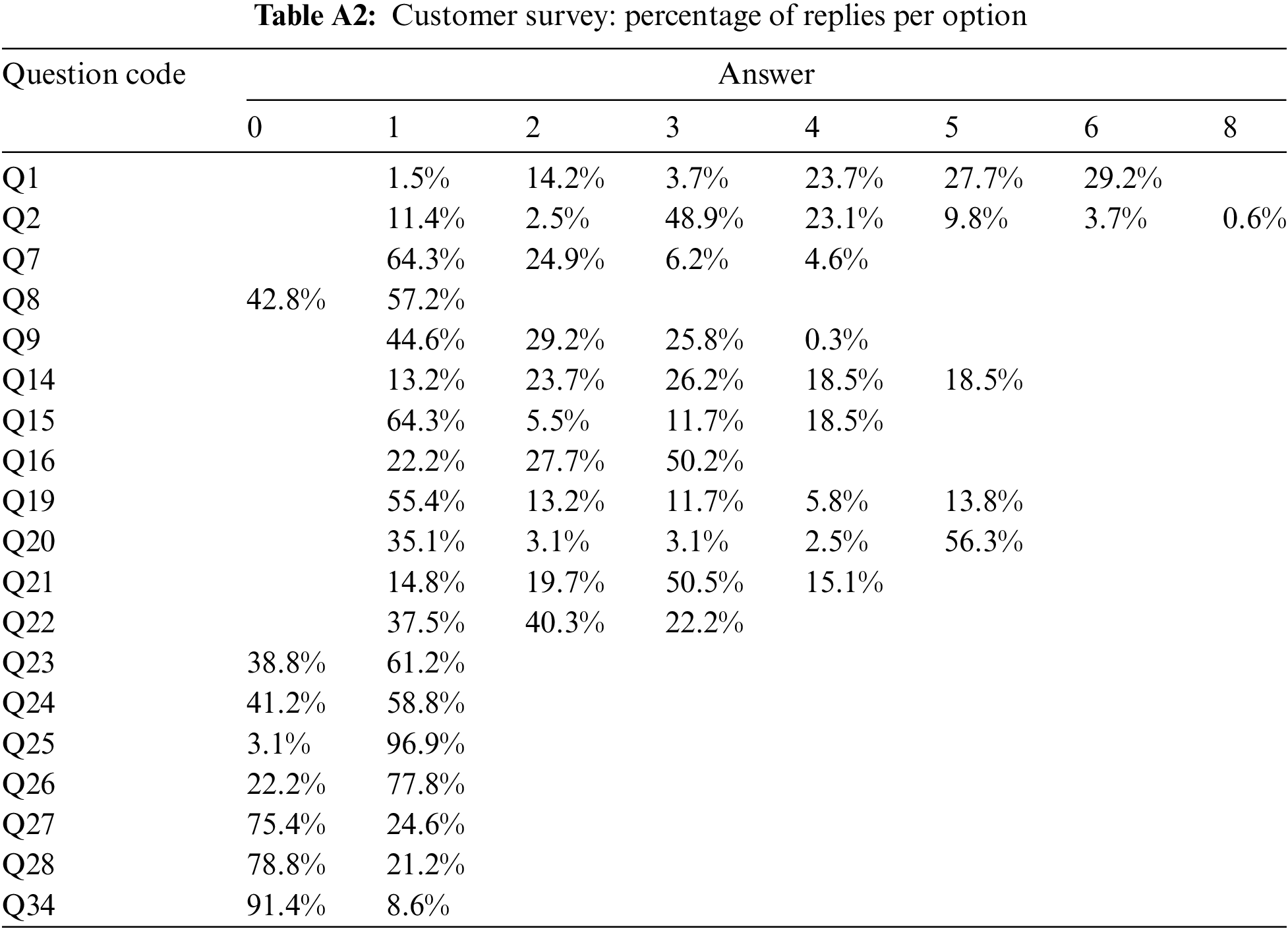
The SME smart meter dataset was filtered to obtain records from 2010, obtaining 484 unique customer codes. Data quality is high: 429 customers (88%) have 100% complete records, 29 (~6%) missed 1 day of data, 22 (~5%) missed 2 days, and only 5 (~1%) missed 1 day worth of data. Missing values were interpolated using Seasonally Split Missing Value Imputation [68]. Items over two-thirds of days with zero consumption have been filtered out from the dataset. The dataset al.so contains a pretrial survey with 92 questions [69], which is utilized to characterize the customer and its facilities as a source of external validation. Tables A1 and A2 in Appendix A show the 16 questions considered for the analysis, given their relevance and the quality and completeness of the answers. The intersection between the clean 2010 smart meter data and the customer characterization embedded in the selected survey questions provides 325 unique customer IDs with a complete set of smart meter data for one year and complete data for external validation.
Each customer time series of 17,520 values (365 days by 48 time points per day) is split into three: a single value representing the average daily energy consumption over the year, a vector of 365 normalized daily energy values totals, and a time series of half-hourly energy use normalized by the total daily energy, as illustrated in Fig. 2. Daily energy shows a right-skewed distribution with an average of ~50 kWh/day. The average daily energy is slightly higher in the winter than in the spring and summer months and shows a clear weekly seasonality. The normalized half-hourly load shape shows an expected average profile with well-defined periods (night, morning, afternoon, and evening) but with a large dispersion among customers.
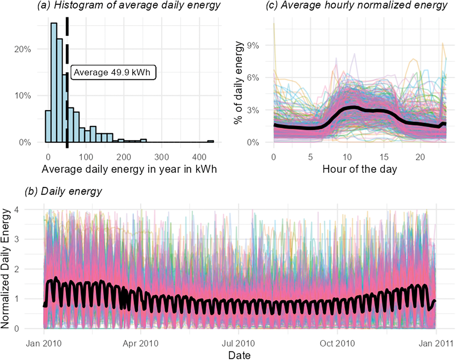
Figure 2: Smart meters time series split
4.2 Block #2: Clustering of Normalized Daily Energy Time Series
Fig. 3 compares different daily energy time series clustering models using Cramer’s V correlation between the categorical vector of the resulting clustering labels and the selected customer attributes as defined in the surveys as an external validation metric. The selected customer attributes are divided into two categories: operational attributes (Q7, Q8, and Q9), which are related to the operational schedules of the SMEs, and equipment attributes (Q23 and Q24), which are related to the existence of thermally sensitive equipment for cooling or heating. Cramer’s V values are represented for all models and each number of clusters, showing the average value of operational and equipment attributes and the total average.
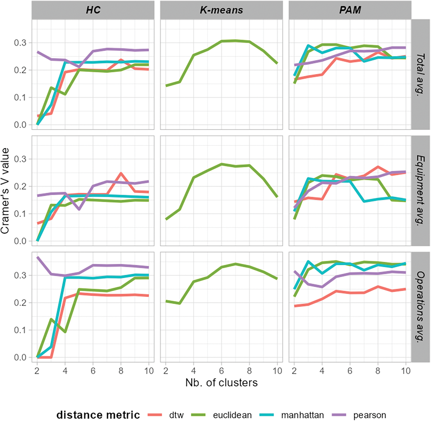
Figure 3: Comparison of clustering methods for daily energy clustering
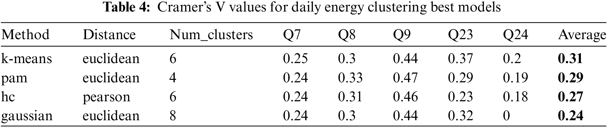
Table 4 details the Cramer’s V values for each attribute for the best model of each method. The PAM model with Euclidean distance is selected as the model that best combines simplicity (only 4 clusters vs. 6 clusters in k-means and HC) with the best results in correlation with operational attributes and the second best in equipment.
4.2.2 Identification of Daily Energy Representatives
Fig. 4 shows the daily energy profiles of the medoids of each cluster for the selected method and distance. Clusters #1 (27% of customers) and #2 (13% of customers) show a similar trend throughout the year, with slightly higher energy use in the winter months, with the difference of a daily variation much higher in the case of Cluster #2. Cluster #4 (26% of customers) also depicts a relatively flat average energy use throughout the year, but with much less variation in daily energy use. Finally, Cluster #3 (34% of customers) illustrates the greatest difference between the summer and winter, with energy use in winter roughly double that in summer.
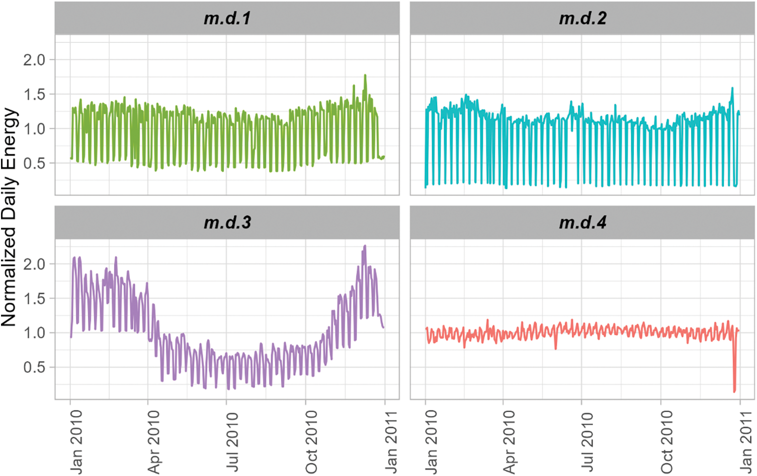
Figure 4: Medoids of each daily time series cluster
4.3 Block #3: Clustering of Normalized Hourly Energy Time Series
4.3.1 Step Function Complexity Reduction per Day-Unit
Fig. 5 illustrates the dimensionality reduction process for a single day of a given customer of the dataset (Customer ID: 1503; Date: 13 October 2010). Considering the average load shape of SME customers, the number of steps considered is five, corresponding to night, morning, lunchtime, afternoon, and evening. In this example, the reduction factor equals ~5.3, the ratio between 48 original time values and nine parameters after the transformation (five steps and four jumps values). This complexity reduction process is conducted for the 365 day-units of each of the 325 customers’ smart meter time series analyzed.
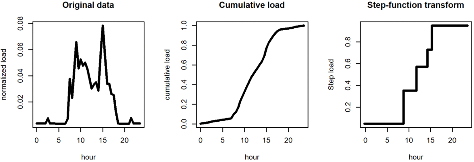
Figure 5: Complexity reduction via cumulative step function transformation
4.3.2 Grid Search to Determine the Best Parameters of the Hourly Energy Clustering Procedure
The hourly clustering procedure described in Section 3.3 requires the choice of three parameters: the number of steps
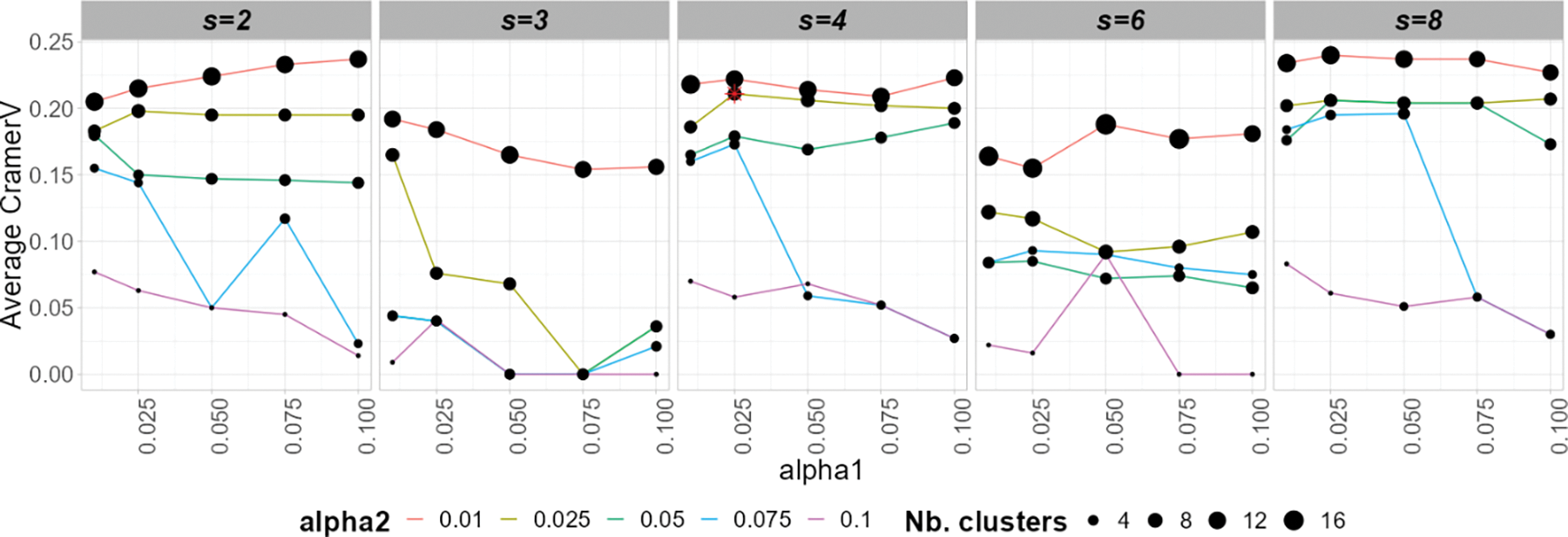
Figure 6: Grid search comparative results to select hourly energy clustering parameters
Fig. 6 indicates that in a single visualization, the effect of the variation of the three input parameters (
Fig. 6 shows the average values of Cramer’s V across the five selected customer attributes: Q7, Q8, and Q9 (operations) and Q23, Q24 (equipment). It is also insightful to differentiate the correlation results for each attribute separately. Fig. 7 depicts the variation of Cramer’s V results per attribute for all models and compares them to the chosen model (in red). The correlation factors are higher for Q24 (presence of cooling equipment) and Q9 (operations during the weekend), and for Q23 (presence of heating equipment) and Q8 (evening operations), the results vary widely, being at the lower end close to zero. The chosen model has correlation factors above the normal variation range for all the attributes considered.
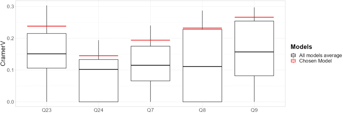
Figure 7: Cramer’s V correlation factor per attribute grid search comparative results
4.3.3 Hourly Clustering #1 and #2: Day-Unit Representatives
Applying the Hourly Clustering #1 procedure with the chosen parameters identifies day-unit representatives per customer, ranging between a median of 5 representatives per customer, a minimum of 2, and a maximum of 12. The computation of internal clustering validation metrics shows good clustering results for Hourly Clustering #1: an average distance reduction of 52% (maximum of 90%) and an average mean silhouette value of 0.33 (maximum 0.91). Hourly Clustering #2 procedure identifies seven standard day-unit hourly profiles, depicted in Fig. 8. Two main categories of profiles can be identified. Most of the customers’ day-units (~73%) show a “standard” SMEs profile, operating during normal business hours (m.2.1 -21%-, m.2.2 -31%- and m.2.3 -21%-). The three clusters in this category differ in the “flatness” of the hourly energy profile, which depends on the relative day vs. night energy use. The second category of SMEs (~26%) has operating hours mainly in the evening or at night (m.2.4 -21%-, m.2.5 -31%- and m.2.6 -21%-). Finally, ~1% of customers’ day-units correspond to 24-h zero energy use profiles (m.2.7). The internal validation metrics for Hourly Clustering #2 achieved are an average distance reduction of 50.3% and an average silhouette value of 0.298 (with a maximum of 0.34).
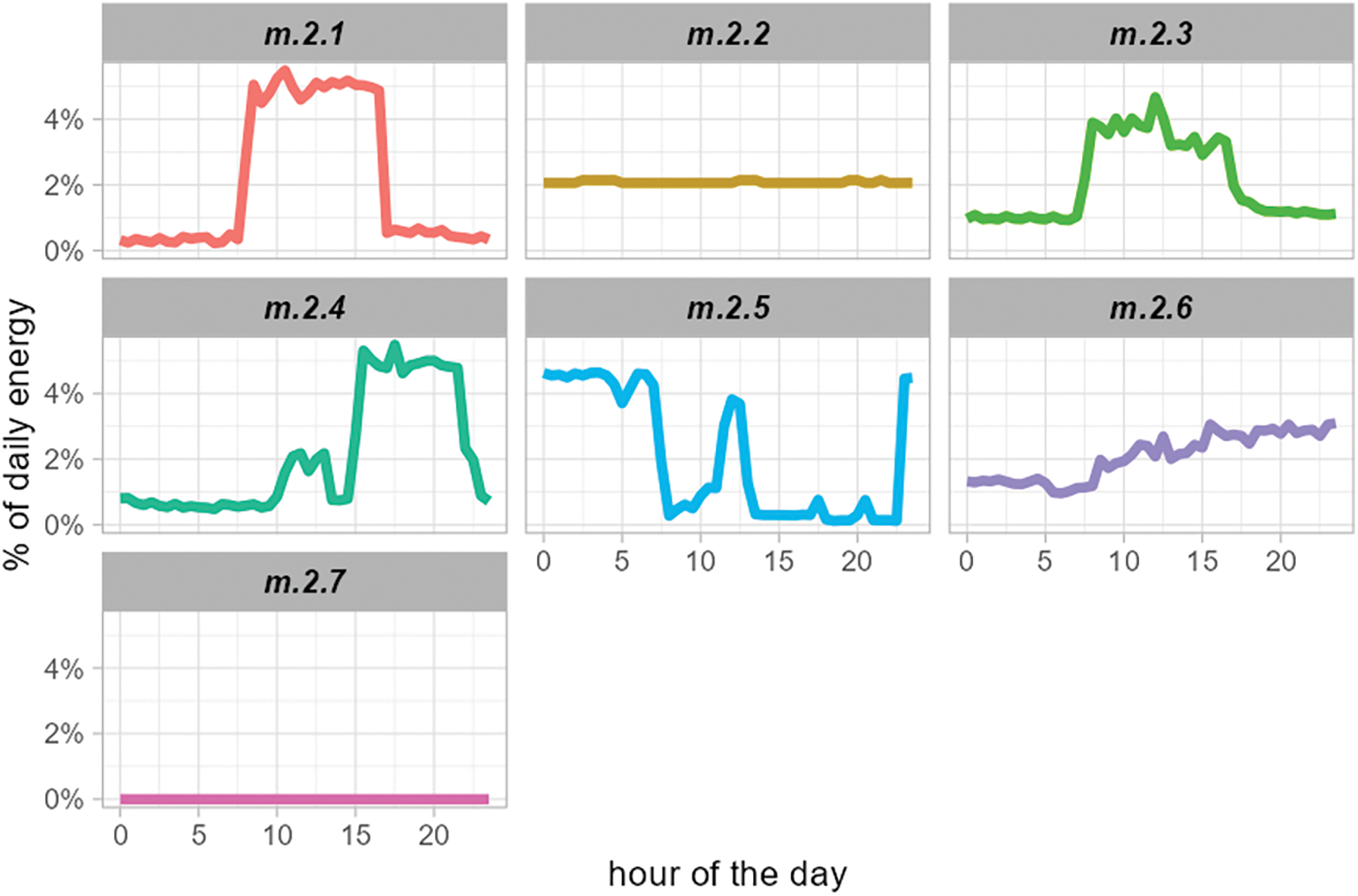
Figure 8: Medoids of Hourly Clustering #2 (standard day-unit hourly profiles)
4.3.4 Comparison of Step-Function Approach for Dimensionality Reduction and Piecewise Aggregate Approximation
Regarding external validation metrics, the clustering results were compared to an alternative complexity reduction technique, the Piecewise Aggregate Approximation (PAA), to verify the contribution of the cumulative step function transformation used in this study. The advantage of the step function approach over PAA is that the periods after the transformation do not have the same value and better reflect the actual temporal behavior of the customer. The cumulative step function approach also avoids arbitrariness in selecting proper time boundaries for preselected periods when using heuristic features for dimensionality reduction (defining the morning period between 9 a.m. and noon). The comparison results show that the step-function approach achieves a ~15% better equipment correlation factor, a similar correlation with operational attributes, and an overall improvement of ~6% in the total correlation for the five attributes selected. However, a better accuracy comes at the price of an increase of ~60% in computation time.
4.3.5 Individual Customer’s Assessment of Hourly Clustering Evolution Over Time
The methodology implemented in this study allows an analysis of the temporal evolution of individual hourly energy use profiles. Several day-unit profiles with a unique time series characterize each customer. Table 5 shows the distribution of the number of Hourly Clustering #2 per customer. The median number of hourly clustering #2 day-unit profiles per customer is 3, with a minimum of 1 (same day-unit profile throughout the year) and a maximum of 6.
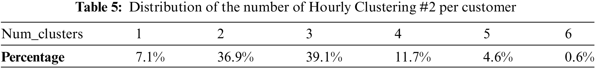
Table 6 shows the percentage of customers where each cluster is more represented. The “standard” profile depicted by clusters m.2.1, m.2.2, and m.2.3 are the most frequent standard days for 76% of customers.
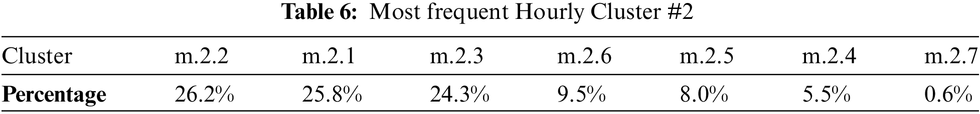
Fig. 9 illustrates the temporal evolution of Hourly Clustering #2 day-unit profiles for a customer. From this rate evolution graph, weekly and seasonal patterns of hourly energy use profile can be detected: profiles #1, #4, and #5 are much more common during weekends (~70% to 90% of these profiles occur during weekends) and specific profiles characterize the summer months (profile #2: ~70% from June to August) and other profiles characterize the winter months (profiles #4 and #5: ~80% to 100% from October to February).
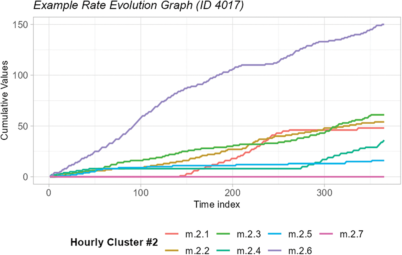
Figure 9: Illustration of Hourly Cluster #2 time evolution profile
4.3.6 Hourly Clustering #3: Customer Segmentation according to Hourly Load-Shape Patterns
Computation of Distance between Hourly Representatives
The distance between each centroid of Hourly Clustering #2 is computed by integrating the function resulting from the difference between the step functions of each pair of centroids to build the dissimilarity matrix
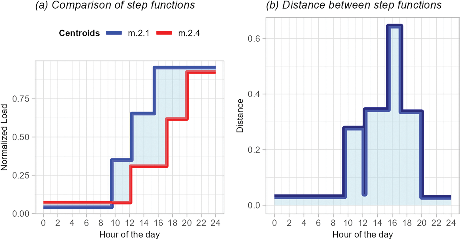
Figure 10: Computation of distance between the step functions of two Hourly Clustering #2 Centroids
Applying this procedure to all the Centroids generates the dissimilarity matrix
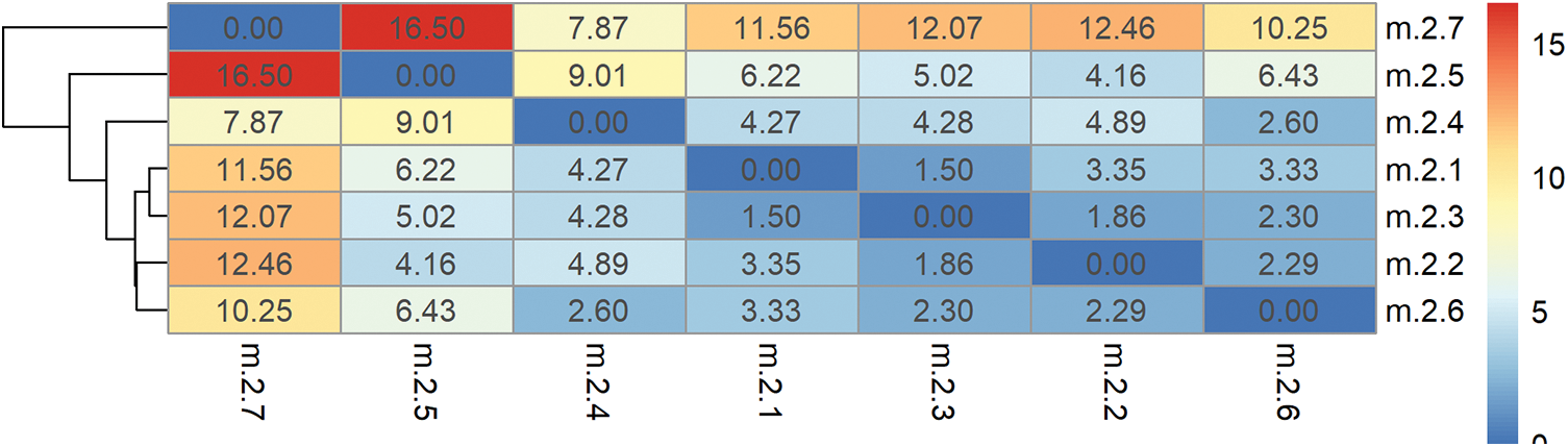
Figure 11: Heatmap of the distance between Hourly Clustering #2 Centroids
Hourly Clustering #3 Results
HC and PAM are applied to two different clustering methods using the distance function defined in equation Eq. (2) as a dissimilarity matrix. The correlation factor Cramer’s V is used again as an external validation metric. Fig. 12 shows the comparative results. HC clustering method with an optimal number of 6 clusters is selected based on visual inspection.
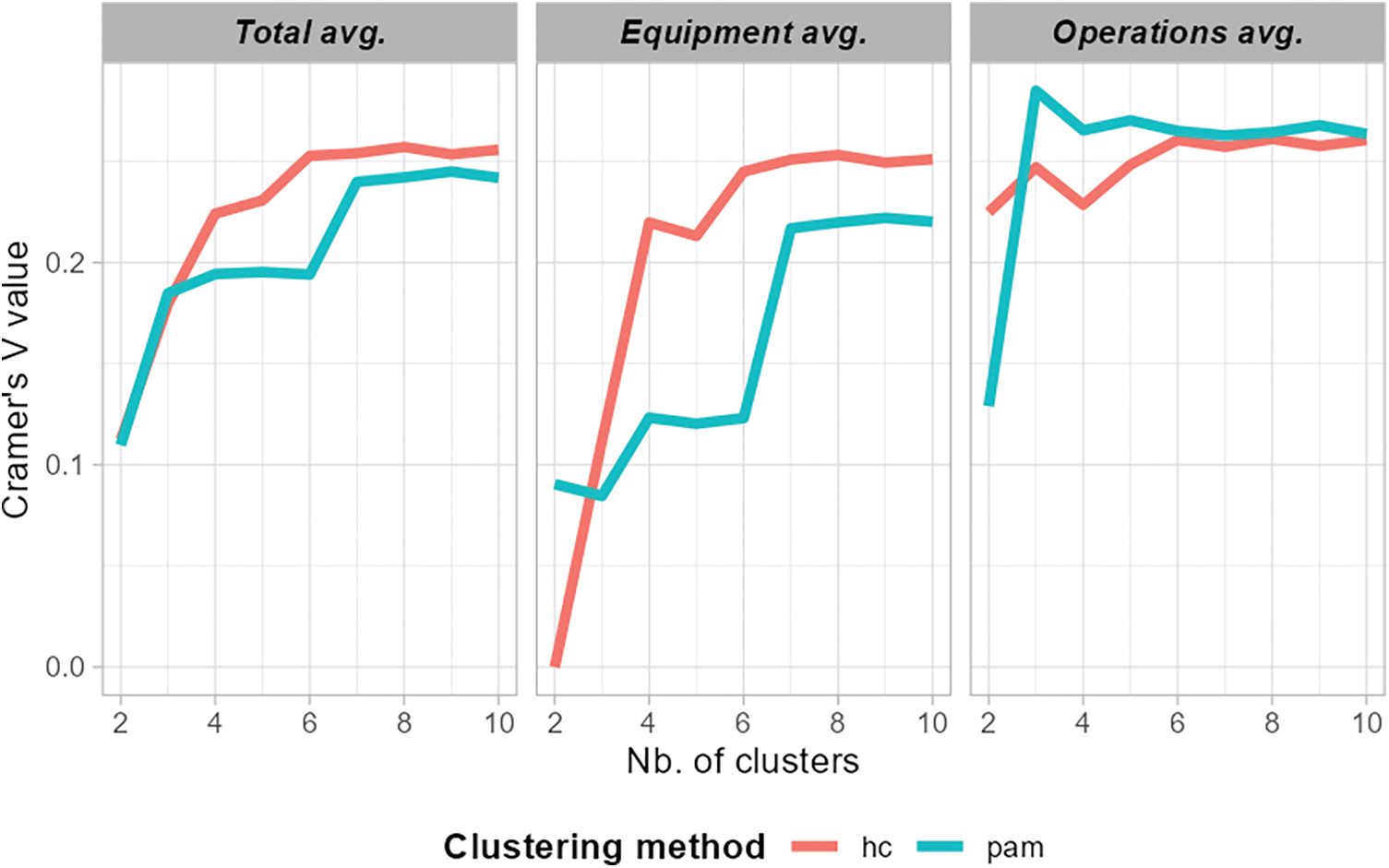
Figure 12: Determining the number of clusters for Hourly Clustering #3
Relationship between Hourly Clustering #2 and #3 Membership
After applying the full clustering procedure, each customer is assigned a single Hourly Clustering #3 cluster and a time series of 365 Hourly Clustering #2 labels. The mosaic plot in Fig. 13 shows the relative share of each customer’s hourly load-shape profile (Hourly Cluster #3) and the proportion of standard day-unit profiles (Hourly Cluster #2), sorted by size. Customer Hourly Clusters #1 to #3 represent ~70% of all customers and are mainly represented by standard day-unit day profiles on days #1 to #3, representing the SMEs operating during normal business hours throughout the day. Customer hourly clusters #4 to #6 represent ~10% of customers each and illustrate SME customers that operate mainly in the evening or at night, each of them having a higher proportion of one of the standard day-unit profiles representing evening or night operations (standard day-unit standard daily profiles days #4 to #6). Standard day-unit profile #7, which has zero daytime energy use, focuses on the hourly profile of customers #4 (8% of the days) and #6 (2% of the days).
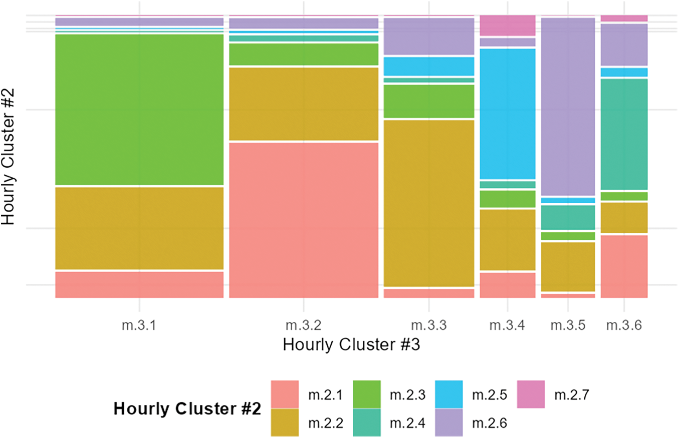
Figure 13: Proportion of standard day-unit profiles in customer hourly profiles
4.4 Block #4: Demand Flexibility Characterization via Time Series Feature Engineering
4.4.1 Daily Clusters’ Characterization with Demand Flexibility Features
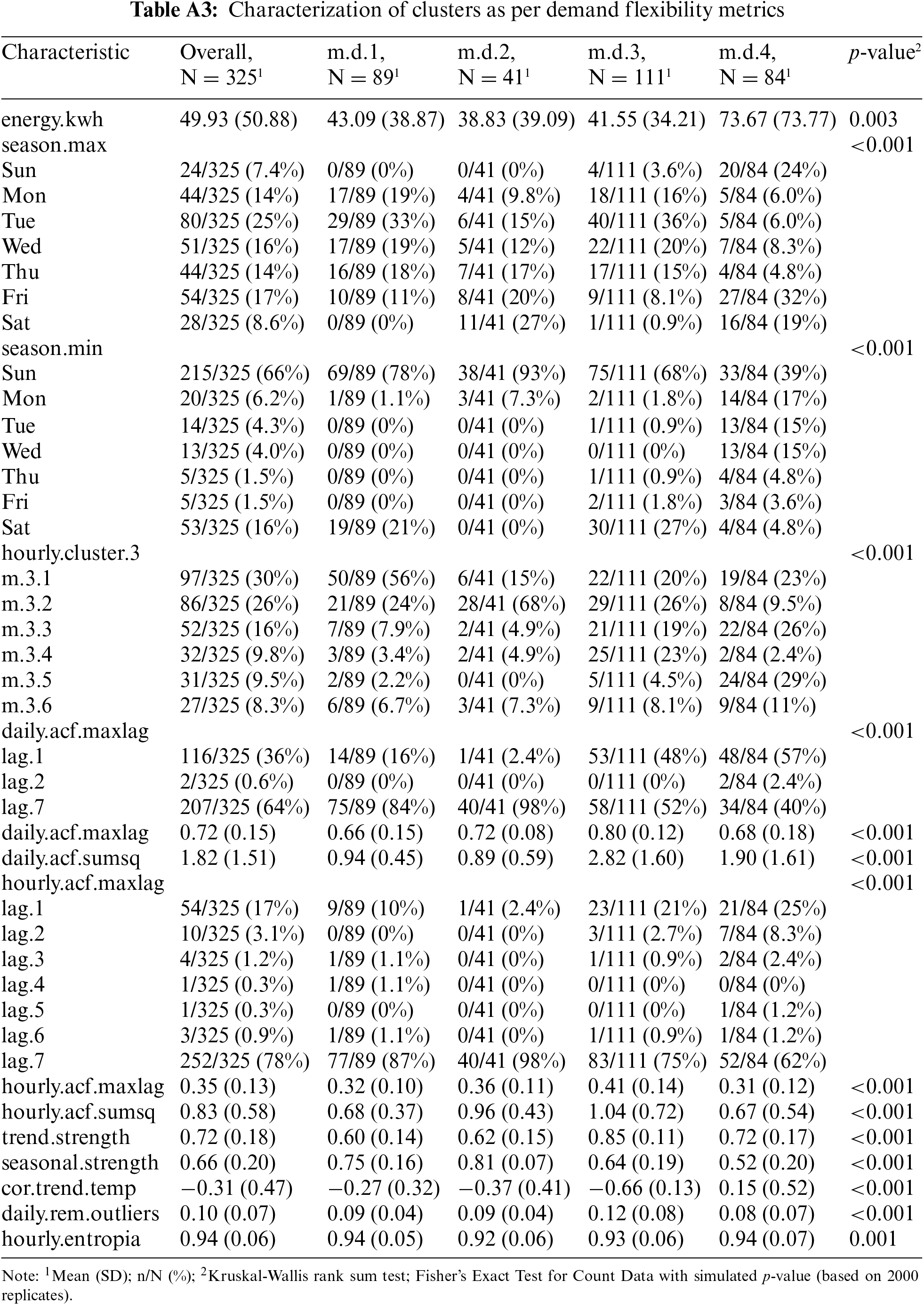
Each customer and cluster are characterized from a demand flexibility perspective by extracting the time series features defined in Table 2. Table A3 shows the distribution patterns of each attribute in the total customer population and the relative distribution for each daily cluster. The p-values of the Kruskal-Wallis rank sum test and Fisher’s Exact Test imply that all features have the statistical significance of each attribute as a cluster differentiation. The m.d.4 daily cluster is characterized by a much higher mean energy use (~50% higher on mean than the average energy of the total population), a higher relative energy use during weekends, a stronger daily energy correlation with a lag of one day, a positive correlation between temperature and relative energy use (higher energy use in the summer months) and slightly larger variation in day-unit hourly clustering profiles. The daily cluster m.d.3 has a lower mean daily energy use, a peak of weekly seasonality concentrated in the middle of the week, and the strongest autocorrelation factor in both daily and hourly time series, with a greater concentration in one-day lags, which implies greater predictability in energy use than average. These daily clusters exhibit the strongest negative correlation with low temperatures and the largest unexplained daily energy variation. Daily Clusters #1 and #2 show similar features in terms of mean energy consumption, lower predictability as measured by autocorrelation factors, low trend strength, around average negative correlation with low temperatures, and lower un-explained daily energy variation. On the other hand, they differ in the weekly seasonal strength, with Daily Cluster #2 being the strongest, the consistency of hourly day-unit series measured by the autocorrelation factor, and the loci of weak seasonality, which is more concentrated on Saturdays in case of Cluster #2. The summary table also shows the relative composition of daily energy clusters in customer hourly load-shape clusters (Hourly Clustering #3). Daily Cluster #1 is dominated by customer Hourly Cluster #1, Daily Cluster #2 has a higher proportion of customer Hourly Cluster #2, and Daily Clusters #3 and #4 have a greater variation in hourly profiles but with a relatively higher proportion of evening and night hourly customer profiles.
4.4.2 Interpretation: Suitability of Clusters for Demand Flexibility Programs
The suitability of each cluster group for demand flexibility programs will depend on the nature of the program. Fig. 14 depicts the variation of critical features (mean plus/minus standard deviation) to define DR suitability following the qualitative framework in Table 3. Clusters #1 and #2 are quite similar regarding their DR suitability. Their high seasonality strength makes them particularly suited to price-based programs, and a percentage of ~9% of outliers in the remainder component will also make them receptive to incentive-based programs. Cluster #3 is the best suited for demand flexibility for both price and incentive-based programs. This Cluster exhibits the highest negative correlation with temperature, high predictability in larger daily and hourly ACF factors, and the highest percentage of outliers in the remainder. Cluster #4 will be the best target for a demand flexibility program focused on-demand control during the summer. Demand during the hottest days can be managed by controlling the set points of thermostatic loads by having the highest mean daily energy and a positive correlation between temperature and daily energy use.
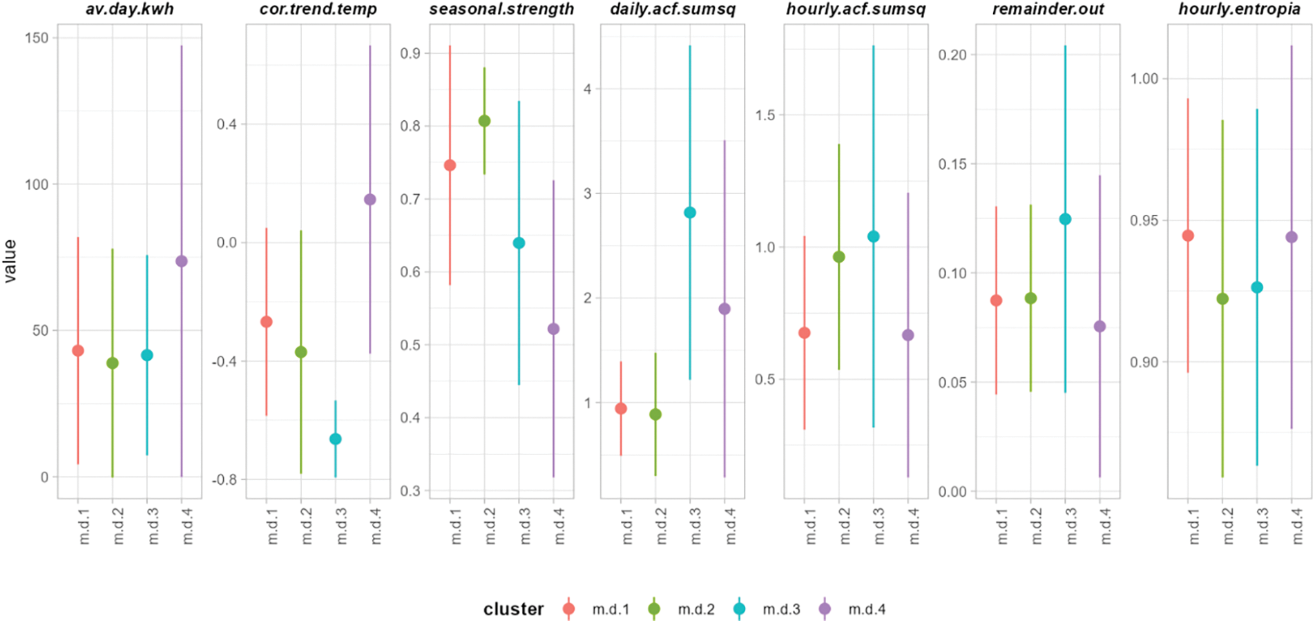
Figure 14: Variation of selected DR features per daily cluster
4.4.3 Daily Clusters’ Characterization with Customer and Building Attributes
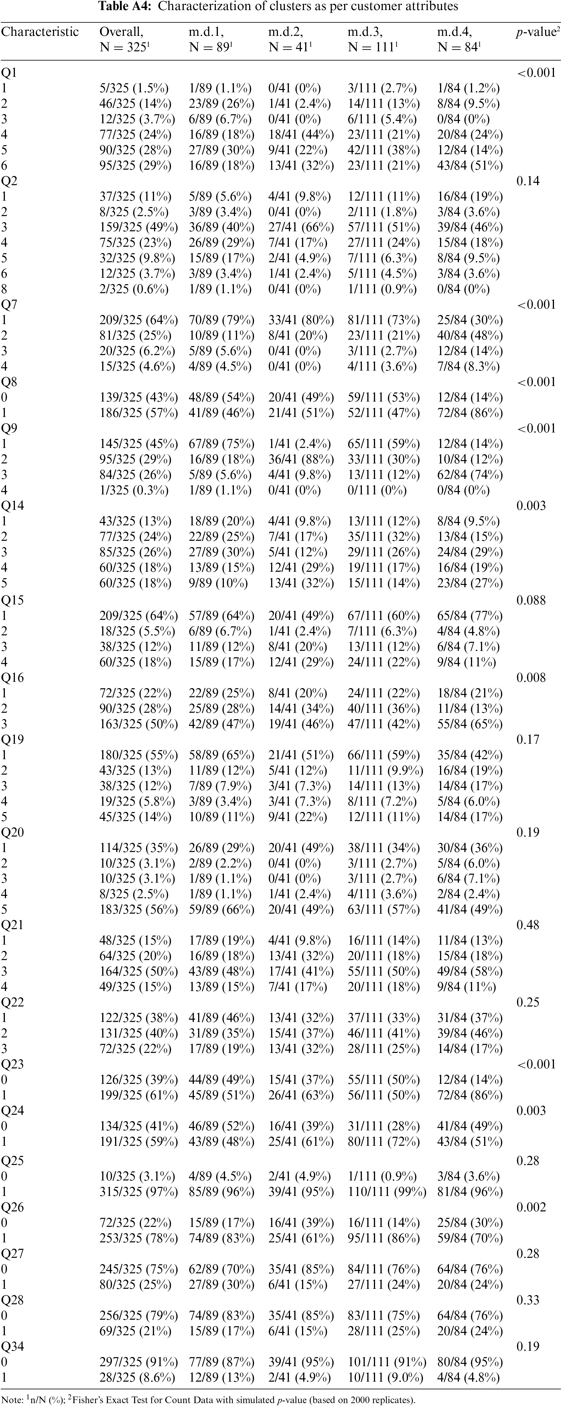
Table A4 in the Appendix A also shows the statistical characterization of the daily energy clusters regarding customer attributes included in the surveys. Only eight customer attributes reveal statistical significance as determinants of the daily energy load shape: business sector (Q1), attributes that define the operations schedule (Q7, Q8, and Q9), the age of the facilities (Q14), the presence of cooling (Q23) and heating (Q24) equipment and the existence of administrative or office equipment (Q26). Daily Cluster #1 has a relatively higher proportion of SMEs in the mining industry, standard business operations during weekdays, and relatively new facilities. Daily Cluster #2 has a relatively higher proportion of SMEs in wholesale trade, standard business operations that also open on Saturdays, older premises, and a relatively lower percentage of office equipment. Daily Cluster #3 is more dominated by professional services, operating standard day hours, with some businesses open in the evenings and mainly on weekdays. The most important attribute is a higher proportion of businesses with heating equipment and, unsurprisingly, with office administrative equipment. Daily Cluster #4 has a more significant proportion of the “others” business sector, primarily extends operations into evenings and weekends, and has the largest proportion of cooling equipment. This cluster can correspond to businesses in the food and catering sectors that use cooling equipment to prevent the deterioration of fresh products. This additional characterization of the daily energy load-shape clusters reinforces the identification of Clusters #3 and #4 with the greatest potential for demand flexibility due to their relatively high consistency in energy use patterns and the presence of equipment temperature-sensitive that can be employed to modify demand according to the system needs.
The multi-step clustering procedure proposed in this study has several advantages over simpler load clustering approaches based on classical dimensionality reduction techniques applied in a single step. First, the 3-way split of smart meter data allows the characterization of distinct time series in different periods (yearly, monthly, weekly, daily, and intra-daily) without loss of information, making this distinction significant for DSM applications. Splitting facilitates a raw data approach to clustering of daily energy time series due to the radical reduction in the number of elements in the daily energy time series data (see Section 3.2). Second, the three-step clustering reduces sequential dimensionality, extracting value and insights at each step. In this way, each customer can be characterized according to the evolution of its membership to Hourly Clustering #2 centroids (see Section 4.3.5), and relevant time series characterization features can be defined using information from each clustering step (see Table 2). Third, staging the identification of the day-unit representatives as medoids at first the local level (customer) and then at the global level (population) radically improves the scalability of the methodology (see Section 3.3.3). In addition, several techniques were utilized to rigorously characterize the interactions between the different elements of the time series split and the results of each clustering stage. For instance, the cross-summary table Table A3 statistically characterizes the relationship between daily cluster results and the average daily energy in kWh and the relationship between Daily Clustering and Hourly Clustering #3. Fig. 13 illustrates the relationship between Hourly Clusters #2 and #3. The relevance of the different identified clusters is tested using a combination of external and internal validation metrics. Daily Clusters and Hourly Clusters #3, representing each customer in the dataset, use a statistically significant external validation metric to ensure alignment with customer attributes important for demand flexibility applications (thermostatic loads and operational schedules in this study). The definition of day-unit hourly profiles that represent each customer (Hourly Clustering #1) and the entire population (Hourly Clustering #2) is based on the reduction of intra-cluster distance. Internal validation metrics show good clustering results: an average reduction of the intra-cluster distance of 52% in Hourly Clustering #1 and 50% in Hourly Clustering #2 and an average silhouette value of 0.33 and 0.298, respectively.
Fig. 15 compares the external validation results using equipment attributes (Q23 and Q24) and simpler single-step k-means to illustrate one of the benefits of a multi-step clustering approach over simpler one-step alternatives. The simpler model has been built using PAA with four steps for dimensionality reduction, averaging the energy use values for each period of the day throughout the year. Energy values were min-max normalized and used as variables in a k-means clustering procedure. Equipment attributes were chosen as a benchmark for two reasons: first because cooling and heating equipment are critical elements in providing demand flexibility; second, the impact of these devices changes over time, depending on the season. The comparative results show better correlations between clusters and equipment are obtained for HC and PAM multi-step models. In addition, the results of the one-step model are less stable than those provided by the multi-step models: the correlation factor shows large oscillations depending on the number of clusters considered.
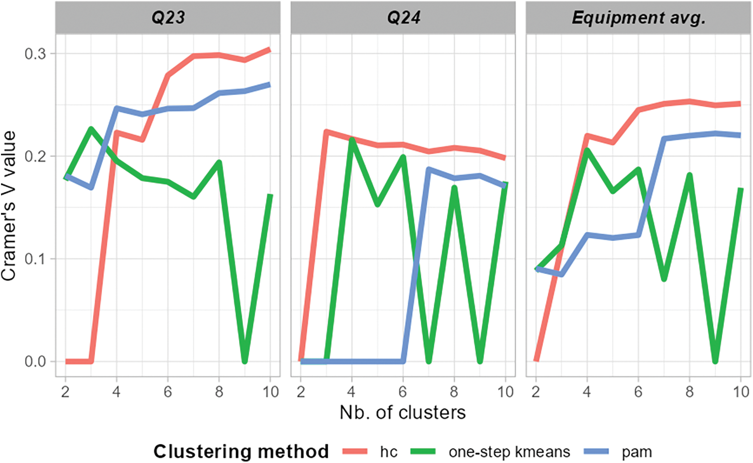
Figure 15: Comparison of multi-step Hourly Clustering and one-step k-means
The characteristics of the Irish CER dataset are a strength in achieving the proposed methodology. The dataset offers detailed, high-quality consumption data over an extended period, beyond the customer surveys that provide behavioral insights. On the one hand, the high granularity allows for capturing subtle variations in consumption patterns. On the other hand, the customer characterization survey provides a comprehensive view of customers. In this way, the combination of both quantitative (energy usage) and qualitative (surveys) data improves segmentation accuracy that simpler datasets would not allow. However, this study also has limitations induced by the chosen dataset that could be addressed in further research. The methodology was designed to be scalable to large datasets using linear methods, staging the k-medoids clustering procedure, and simple matrix computation for distance computation in Hourly Clustering #3 (Section 3.3.3). However, the methodology should also be applied to larger datasets to assess the impact of the computing setup and the application of big data management techniques on the scalability and computing efficiency of the methodology. On the one hand, scaling the methodology to larger data sets may involve using more advanced computing infrastructure, such as distributed computing or cloud-based platforms. On the other hand, the methodology can be extended to different customer segments by introducing additional parameters to capture the characteristics of each segment or by incorporating feedback loops where insights from segment-specific analyses can refine the overall methodology. Applying the step-function approach can also question the scalability of the methodology. The step-function approach outperforms PAA as it can more accurately capture variations in time-series data. In this case, it avoids arbitrariness in selecting proper time boundaries for preselected periods. However, it increases the computational burden. Therefore, there is a trade-off between accuracy and computational cost. Several potential solutions could be implemented to address this problem. For instance, parallel computing or optimization techniques can be utilized to reduce processing time, or a hybrid approach combining the step-function approach with PAA, using PAA for the initial rough segmentation and the step-function approach to refine the most critical sections.
The other limitation regards the potential biases in the dataset used for this study. The dataset’s relatively small size can question this sample’s representativeness concerning the whole population of SME customers in Ireland. In addition, the customer selection process for the Irish trial is unknown; therefore, the dataset could overrepresent or misrepresent specific customer segments depending on how the enrolment process was conducted. Applying the methodology to several datasets from different regions and customer segments and comparing the results would contribute to confirming robustness.
The demand flexibility potential of a customer was characterized by 16 indicators organized around four key categories: Energy (E), Temporal patterns (T), Consistency (C), and Variability (V). The amount of energy that a given customer can supply to the system depends on the total energy consumed (E), the temporal structure of trend and seasonality patterns (T), the degree of predictability in energy consumption (C), and the “free” energy available measured as un-explained variation in energy use (V). The proposed demand flexibility indicators define the structure of the numeric (daily energy) and categorical (hourly patterns of energy use) time series for each customer. Table A3 in Appendix A lists each indicator’s relative importance in the clustering process. The p-value metric allows for benchmarking of the relative significance of each metric in the clustering results, where a lower value represents greater importance. The relative significance of each demand flexibility metric in the clustering results is also illustrated in Fig. 14. Utilities and energy services companies may use this clustering methodology for several purposes. As illustrated in this study, the smart meter time series splitting and the sequential clustering methodology would allow energy companies to engage similar customers and groups of customers for price and incentive-based demand flexibility programs. The 3-step clustering procedure could also be used to propose hyper-personalized pricing schemes to customers; based on the evolution of the standard daily-unit profile pattern (Section 4.3.5), customized pricing structures can be automatically defined per customer considering patterns of energy use at the annual, monthly, weekly, daily and intra-day level. Daily and Hourly Clustering can also be used for large-scale load forecasting over short, medium, and long-term horizons. Instead of computing the energy forecast from the raw data of each customer, which is highly demanding in terms of computing power when dealing with real-life datasets, the load forecast can be applied to the representative elements in each clustering stage and then generalized to each of the members per cluster. Finally, additional characterization of the clusters according to customer attributes, such as operational schedules, presence of equipment, or socioeconomic variables, would allow a scenario-like forecast of long-term load profiles according to potential evolutions of customer attributes, such for example, greater penetration of specific equipment such as EVs or heat pumps or a structural change in socio-economic variables such as the typology and size of SMEs or the number of members per household.
The multi-step clustering procedure applied to a dataset of 325 SME customers successfully identifies energy use load-shape patterns at both daily and intra-daily (hourly) levels. In addition, extracting relevant features from time series allows for characterizing the demand flexibility of customers and corresponding clusters along the axis of available energy, temporal patterns, consistency, and variability. The clustering procedure applies a sequential complexity reduction, generating deep knowledge at each step. First, splitting the daily and hourly normalized time series allows a raw-data approach to the daily energy times series without loss of information. Second, the three-step intraday hourly energy time series progressively identifies load-shape patterns, individually and collectively. The first step of the hourly clustering step identifies day-unit representatives per customer and characterizes the variation of load shapes per customer. The second step of hourly clustering defines standard day-unit load-shape profiles, representatives of the entire population. The third step of hourly clustering segments customers into six hourly clustering profiles, considering the evolution of the standard profiles over time. The methodology introduces three innovative techniques into this clustering procedure: (1) a step-function approach for complexity reduction, (2) correlation with customer attributes as an external clustering validation metric, and (3) a matrix-based ad-hoc distance metric to segment customers based on hourly load-shape patterns. In addition, the correlation between customer attributes embedded in surveys and daily and hourly cluster labels is employed to identify statistically significant determinants of load shape in energy use. The application of the methodology includes the selection of critical parameters using grid search and the comparison of distances and clustering methods to ensure the robustness of the results. The methodology is designed to be computationally effective and scalable to a larger number of customers.
Further work can extend the methodology to larger datasets, including households, and explore applying the clustering results beyond the demand flexibility characterization. Correlation analysis between clusters based on load-shape, time series features, and customer attributes opens the door to future research on customer attribute inference from load-shape time series features extraction or the mirror-supervised problem of predicting load-shape patterns from customer attributes.
Acknowledgement: This work was partly supported by the Spanish Ministry of Science and Innovation under Projects PID2022-137680OB-C32 and PID2022-139187OB-I00. This publication is also supported by Iberdrola S. A. as part of its innovation department research studies. Its contents are solely the authors’ responsibility and do not necessarily represent the official views of Iberdrola Group. The primary author thanks Iberdrola for its support in providing a virtual machine to undertake computer simulations.
Funding Statement: The authors received no specific funding for this study.
Author Contributions: Conceptualization, Santiago Bañales; methodology, Santiago Bañales; supervision, Raquel Dormido and Natividad Duro; writing—original draft, Santiago Bañales; writing—review and editing, Raquel Dormido and Natividad Duro. All authors reviewed the results and approved the final version of the manuscript.
Availability of Data and Materials: The Irish Smart Seter Trial CER dataset has been accessed via the Irish Social Science Data Archive—www.ucd.ie/issda (accessed on 30 August 2024) in accordance with the terms of use of the License agreement. Copyright and all other intellectual property rights in the data and associated documentation are vested in the original data creators or depositors. The authors of this paper acknowledge the work of the original data creators, depositors, copyright holders, and the ISSDA and declare that those who carried out the original analysis and collection of the data bear no responsibility for further analysis or interpretation of it. Copyright and all other intellectual property rights in the data and associated documentation are vested in the original data creators or depositors. Weather data has been obtained from the Irish Meteorological Service (Met Éireann) historical data service (source www.met.ie) (accessed on 30 August 2024). Copyright Met Éireann. These data are published under Creative Commons Attribution 4.0 International (CC BY 4.0). https://creativecommons.org/licenses/by/4.0/ (accessed on 30 August 2024). Disclaimer: Met Éireann does not accept any liability whatsoever for any error or omission in the data, their availability, or for any loss or damage arising from their use.
Ethics Approval: Not applicable.
Conflicts of Interest: The authors declare no conflicts of interest to report regarding the present study.
References
1. COP26. The glasgow climate pact. In: UN Climate Change Conference, UK, 2021. Available from: https://ukcop26.org/wp-content/uploads/2021/11/COP26-Presidency-Outcomes-The-Climate-Pact.pdf. [Accessed 2024]. [Google Scholar]
2. Pee LG, Pan SL. Climate-intelligent cities and resilient urbanisation: challenges and opportunities for information research. Int J Inf Manage. 2022;63:102446. doi:10.1016/j.ijinfomgt.2021.102446. [Google Scholar] [CrossRef]
3. Brown D, Hall S, Davis ME. Prosumers in the post subsidy era: an exploration of new prosumer business models in the UK. Energy Policy. 2019;135:110984. doi:10.1016/j.enpol.2019.110984. [Google Scholar] [CrossRef]
4. Di Silvestre ML, Ippolito MG, Sanseverino ER, Sciumè G, Vasile A. Energy self-consumers and renewable energy communities in Italy: new actors of the electric power systems. Renew Sustain Energy Rev. 2021;151:111565. doi:10.1016/j.rser.2021.111565. [Google Scholar] [CrossRef]
5. Zapata Riveros J, Kubli M, Ulli-Beer S. Prosumer communities as strategic allies for electric utilities: exploring future decentralization trends in Switzerland. Energy Res Soc Sci. 2019;57:101219. doi:10.1016/j.erss.2019.101219. [Google Scholar] [CrossRef]
6. Moura R, Brito MC. Prosumer aggregation policies, country experience and business models. Energy Policy. 2019;132:820–30. [Google Scholar]
7. Bañales S. The enabling impact of digital technologies on distributed energy resources integration. J Renew Sustain Energy. 2020;12(4):045301. doi:10.1016/j.enpol.2019.06.053. [Google Scholar] [CrossRef]
8. Leiva J, Palacios A, Aguado JA. Smart metering trends, implications and necessities: a policy review. Renew Sustain Energ Rev. 2016;55:227–33. doi:10.1016/j.rser.2015.11.002. [Google Scholar] [CrossRef]
9. Pitì A, Verticale G, Rottondi C, Capone A, Lo Schiavo L. The role of smart meters in enabling real-time energy services for households: the Italian case. Energies. 2017;10(2):199. doi:10.3390/en10020199. [Google Scholar] [CrossRef]
10. Glass E, Glass V. Power to the prosumer: a transformative utility rate reform proposal that is fair and efficient. Electr J. 2021;34(9):107023. doi:10.1016/j.tej.2021.107023. [Google Scholar] [CrossRef]
11. Donaldson DL, Jayaweera D. Effective solar prosumer identification using net smart meter data. Int J Electr Power Energy Syst. 2020;118:105823. doi:10.1016/j.ijepes.2020.105823. [Google Scholar] [CrossRef]
12. Talei H, Benhaddou D, Gamarra C, Benbrahim H, Essaaidi M. Smart building energy inefficiencies detection through time series analysis and unsupervised machine learning. Energies. 2021;14(19):6042. doi:10.3390/en14196042. [Google Scholar] [CrossRef]
13. Pressmair G, Amann C, Leutgöb K. Business models for demand response: exploring the economic limits for small-and medium-sized prosumers. Energies. 2021;14(21):7085. doi:10.3390/en14217085. [Google Scholar] [CrossRef]
14. Wang Y, Chen Q, Hong T, Kang C. Review of smart meter data analytics: applications, methodologies, and challenges. IEEE Trans Smart Grid. 2019;10(3):3125–48. doi:10.1109/TSG.2018.2818167. [Google Scholar] [CrossRef]
15. Si C, Xu S, Wan C, Chen D, Cui W, Zhao J. Electric load clustering in smart grid: methodologies, applications, and future trends. J Mod Power Syst Clean Energy. 2021;9(2):237–52. doi:10.35833/MPCE.2020.000472. [Google Scholar] [CrossRef]
16. Rajabi A, Eskandari M, Ghadi MJ, Li L, Zhang J, Siano P. A comparative study of clustering techniques for electrical load pattern segmentation. Renew Sustain Energ Rev. 2020;120:109628. doi:10.1016/j.rser.2019.109628. [Google Scholar] [CrossRef]
17. Forero-Quintero JF, Villafáfila-Robles R, Barja-Martinez S, Munné-Collado I, Olivella-Rosell P, Montesinos-Miracle D. Profitability analysis on demand-side flexibility: a review. Renew Sustain Energ Rev. 2022;169:112906. doi:10.1016/j.rser.2022.112906. [Google Scholar] [CrossRef]
18. Villar J, Bessa R, Matos M. Flexibility products and markets: literature review. Electric Power Syst Res. 2018;154:329–40. [Google Scholar]
19. Gils HC. Assessment of the theoretical demand response potential in Europe. Energy. 2014;67:1–18. doi:10.1016/j.energy.2014.02.019. [Google Scholar] [CrossRef]
20. IEA. Policy pathway powering SMEs to catalyse economic growth accelerating energy efficiency in small and medium-sized enterprises policy pathway; 2015. Available from: https://www.iea.org/publications/freepublications/publication/SME_2015.pdf. [Accessed 2024]. [Google Scholar]
21. Reuter S, Lackner P, Brandl G. Leap 4 SME: mapping SMEs in Europe—data collection, analysis and methodologies for estimating energy consumptions at Country levels; 2021. Available from: www.leap4sme.eu. [Accessed 2024]. [Google Scholar]
22. SEAI. SME guide to energy efficiency. London: Sustainable energy authority for Ireland, 2017. Available from: https://www.seai.ie/sites/default/files/publications/SME-Guide-to-Energy-Efficiency.pdf. [Accessed 2022]. [Google Scholar]
23. Syed D, Abu-Rub H, Ghrayeb A, Refaat SS, Houchati M, Bouhali O. Deep learning-based short-term load forecasting approach in smart grid with clustering and consumption pattern recognition. IEEE Access. 2021;9:54992–5008. doi:10.1109/ACCESS.2021.3071654. [Google Scholar] [CrossRef]
24. Kawoosa AI, Prashar D, Faheem M, Jha N, Khan AA. Using machine learning ensemble method for detection of energy theft in smart meters. IET Gener, Transm Dis. 2023;17(21):4794–809. doi:10.1049/gtd2.12997. [Google Scholar] [CrossRef]
25. Antonopoulos I, Robu V, Couraud B, Kirli D, Norbu S, Kiprakis A, et al. Artificial intelligence and machine learning approaches to energy demand-side response: a systematic review. Renew Sustain Energ Rev. 2020;130:109899. doi:10.1016/j.rser.2020.109899. [Google Scholar] [CrossRef]
26. Warren Liao T. Clustering of time series data—a survey. Pattern Recognit. 2005;38(11):1857–74. doi:10.1016/j.patcog.2005.01.025. [Google Scholar] [CrossRef]
27. Aghabozorgi S, Seyed Shirkhorshidi A, Ying Wah T. Time-series clustering—a decade review. Inf Syst. 2015;53(12):16–38. doi:10.1016/j.is.2015.04.007. [Google Scholar] [CrossRef]
28. Bañales S, Dormido R, Duro N. Smart meters time series clustering for demand response applications in the context of high penetration of renewable energy resources. Energies. 2021;14(12):3458. doi:10.3390/en14123458. [Google Scholar] [CrossRef]
29. Michalakopoulos V, Sarmas E, Papias I, Skaloumpakas P, Marinakis V, Doukas H. A machine learning-based framework for clustering residential electricity load profiles to enhance demand response programs. Appl Energy. 2024;361(4):122943. doi:10.1016/j.apenergy.2024.122943. [Google Scholar] [CrossRef]
30. Wen L, Zhou K, Yang S. A shape-based clustering method for pattern recognition of residential electricity consumption. J Clean Prod. 2019;212(2):475–88. doi:10.1016/j.jclepro.2018.12.067. [Google Scholar] [CrossRef]
31. Liang H, Ma J. Develop load shape dictionary through efficient clustering based on elastic dissimilarity measure. IEEE Trans Smart Grid. 2021;12(1):442–52. [Google Scholar]
32. Tureczek AM, Nielsen PS. Structured literature review of electricity consumption classification using smart meter data. Energies. 2017;10(5):584. doi:10.3390/en10050584. [Google Scholar] [CrossRef]
33. Liu C, Wang X, Huang Y, Liu Y, Li R, Li Y, et al. A moving shape-based robust fuzzy K-modes clustering algorithm for electricity profiles. Elect Power Syst Res. 2020;187:106425. doi:10.1016/j.epsr.2020.106425. [Google Scholar] [CrossRef]
34. Sandels C, Kempe M, Brolin M, Mannikoff A. Clustering residential customers with smart meter data using a data analytic approach—external validation and robustness analysis. In: 2019 9th International Conference on Power and Energy Systems, 2019; Perth, Australia. [Google Scholar]
35. Kushan C, Kowli A. New perspectives on clustering for demand response. In: Jørgensen BN, da Silva LCP, Ma Z, editors. Energy informatics. Cham: Springer Nature Switzerland; 2024. p. 175–91. [Google Scholar]
36. Laurinec P, Lucká M. Comparison of representations of time series for clustering smart meter data. In: Lecture notes in engineering and computer science, Hong Kong, China: Newswood Limited, 2016. p. 458–63. [Google Scholar]
37. Laurinec P, Lucká M. Interpretable multiple data streams clustering with clipped streams representation for the improvement of electricity consumption forecasting. Data Min Knowl Discov. 2019;33(2):413–45. doi:10.1007/s10618-018-0598-2. [Google Scholar] [CrossRef]
38. Gajowniczek K, Bator M, Ząbkowski T. Whole time series data streams clustering: dynamic profiling of the electricity consumption. Entropy. 2020;22(12):1–35. doi:10.3390/e22121414. [Google Scholar] [PubMed] [CrossRef]
39. Wang Y, Bennani IL, Liu X, Sun M, Zhou Y. Electricity consumer characteristics identification: a federated learning approach. IEEE Trans Smart Grid. 2021;12(4):3637–47. doi:10.1109/TSG.2021.3066577. [Google Scholar] [CrossRef]
40. Alonso AM, Nogales FJ, Ruiz C. Hierarchical clustering for smart meter electricity loads based on quantile autocovariances. IEEE Trans Smart Grid. 2020;11(5):4522–30. doi:10.1109/TSG.2020.2991316. [Google Scholar] [CrossRef]
41. Tureczek A, Nielsen PS, Madsen H. Electricity consumption clustering using smart meter data. Energies. 2018;11(4):859. doi:10.3390/en11040859. [Google Scholar] [CrossRef]
42. Eskandarnia E, Al-Ammal H, Ksantini R, Hammad M. Deep learning techniques for smart meter data analytics: a review. SN Comput Sci. 2022;3(3):243. doi:10.1007/s42979-022-01161-6. [Google Scholar] [CrossRef]
43. Eskandarnia E, Al-Ammal HM, Ksantini R. An embedded deep-clustering-based load profiling framework. Sustain Cities Soc. 2022;78:103618. doi:10.1016/j.scs.2021.103618. [Google Scholar] [CrossRef]
44. Xiao JW, Xie Y, Fang H, Wang YW. A new deep clustering method with application to customer selection for demand response program. Int J Electr Power Energy Syst. 2023;150:109072. doi:10.1016/j.ijepes.2023.109072. [Google Scholar] [CrossRef]
45. Sandoval Guzmán B, Barocio Espejo E, Elser M, Korba P, Segundo Sevilla FR. A hybrid clustering approach for electrical load profiles considering weather conditions based on matrix-tensor decomposition. Sustain Energy, Grids Netw. 2024;38:101326. doi:10.1016/j.segan.2024.101326. [Google Scholar] [CrossRef]
46. Wen H, Liu X, Yang M, Lei B, Xu C, Chen Z. A novel approach for identifying customer groups for personalized demand-side management services using household socio-demographic data. Energy. 2024;286:129593. doi:10.1016/j.energy.2023.129593. [Google Scholar] [CrossRef]
47. Schaffer M, Vera-Valdés JE, Marszal-Pomianowska A. Exploring smart heat meter data: a co-clustering driven approach to analyse the energy use of single-family houses. Appl Energy. 2024;371:123586. doi:10.1016/j.apenergy.2024.123586. [Google Scholar] [CrossRef]
48. Vahedi S, Zhao L. Distributed auto-clustering for residential load profiling using AMI data from the U.S. High Plains. IEEE Trans Smart Grid. 2023;14(6):4530–41. doi:10.1109/TSG.2023.3253824. [Google Scholar] [CrossRef]
49. Li Z, Zhang Y, Ai Q. Shape-based clustering for demand response potential evaluation: a perspective of comprehensive evaluation metrics. Sustain Energy Grids Netw. 2023;36:101213. doi:10.1016/j.segan.2023.101213. [Google Scholar] [CrossRef]
50. Pullinger M, Zapata-Webborn E, Kilgour J, Elam S, Few J, Goddard N, et al. Capturing variation in daily energy demand profiles over time with cluster analysis in British homes (September 2019–August 2022). Appl Energy. 2024;360:122683. doi:10.1016/j.apenergy.2024.122683. [Google Scholar] [CrossRef]
51. Zhan S, Liu Z, Chong A, Yan D. Building categorization revisited: a clustering-based approach to using smart meter data for building energy benchmarking. Appl Energy. 2020;269:114920. doi:10.1016/j.apenergy.2020.114920. [Google Scholar] [CrossRef]
52. Mets K, Depuydt F, Develder C. Two-stage load pattern clustering using fast wavelet transformation. IEEE Trans Smart Grid. 2016;7(5):2250–2259. doi:10.1109/TSG.2015.2446935. [Google Scholar] [CrossRef]
53. Fang H, Xiao JW, Wang YW, Chung CY. A new binary encoding method for energy consumption patterns quantification. IEEE Trans Instrum Meas. 2024;73:1–12. [Google Scholar]
54. Wang L, Narayanan V, Yu YC, Park Y, Li JS. A nested two-stage clustering method for structured temporal sequence data. Knowl Inf Syst. 2021;63(7):1627–62. doi:10.1007/s10115-021-01578-0. [Google Scholar] [CrossRef]
55. Afzalan M, Jazizadeh F, Eldardiry H. Two-stage clustering of household electricity load shapes for improved temporal pattern representation. IEEE Access. 2021;9:151667–80. doi:10.1109/ACCESS.2021.3122082. [Google Scholar] [CrossRef]
56. R Core Team. R: a language and environment for statistical computing. Vienna, Austria; R Foundation for Statistical Computing; 2020, Available from: https://www.r-project.org/. [Accessed 2024]. [Google Scholar]
57. Harald C. Mathematical methods of statistics. Princeton: Princeton University Press; 1946. [Google Scholar]
58. Frick K, Munk A, Sieling H. Multiscale change point inference. J R Stat Soc Ser B Stat Methodol. 2014;76(3):495–580. [Google Scholar]
59. Schubert E, Rousseeuw PJ. Fast and eager k-medoids clustering: o(k) runtime improvement of the PAM, CLARA, and CLARANS algorithms. Inf Syst. 2021;101:101804. doi:10.1016/j.is.2021.101804. [Google Scholar] [CrossRef]
60. Xu D, Tian Y. A comprehensive survey of clustering algorithms. Ann Data Sci. 2015;2(2):165–93. doi:10.1007/s40745-015-0040-1. [Google Scholar] [CrossRef]
61. Kathirgamanathan A, Péan T, Zhang K, De Rosa M, Salom J, Kummert M, et al. Towards standardising market-independent indicators for quantifying energy flexibility in buildings. Energy Build. 2020;220:110027. doi:10.1016/j.enbuild.2020.110027. [Google Scholar] [CrossRef]
62. Luo Z, Peng J, Cao J, Yin R, Zou B, Tan Y et al. Demand flexibility of residential buildings: definitions, flexible loads, and quantification methods. Engineering. 2022;16:123–40. doi:10.1016/j.eng.2022.01.010. [Google Scholar] [CrossRef]
63. Pelekis S, Pipergias A, Karakolis E, Mouzakitis S, Santori F, Ghoreishi M et al. Targeted demand response for flexible energy communities using clustering techniques. Sustain Energy, Grids Netw. 2023;36:101134. doi:10.1016/j.segan.2023.101134. [Google Scholar] [CrossRef]
64. Cleveland RB, Cleveland WS, McRae JE, Terpenning I. STL: a seasonal-trend decomposition procedure based on loess (with discussion). J Off Stat. 1990;6:3–73. [Google Scholar]
65. Hyndman RJ, Athanasopoulos G. Forecasting: principles and practice. 3rd ed. Melbourne, Australia: OTexts; 2021. Available from: OTexts.com/fpp3. [Accessed 2024]. [Google Scholar]
66. López-Oriona Á, Vilar JA. Analyzing categorical time series with the R package ctsfeatures. J Comput Sci. 2024;76:102233. doi:10.1016/j.jocs.2024.102233. [Google Scholar] [CrossRef]
67. Commission for Energy Regulation (CER). CER smart metering project—electricity customer behaviour trial, 2009–2010. 1st ed. Ireland: Irish Social Science Data Archive. 2012. [Google Scholar]
68. Moritz S, Bartz-Beielstein T. Time series missing value imputation in R. R J. 2017;9(1):207–18. doi:10.32614/RJ-2017-009. [Google Scholar] [CrossRef]
69. Commission for Energy Regulation (CER). SME pre-trial survey questionnaire. In: CER smart metering project—electricity customer behaviour trial, 2009–2010. 1st ed. Ireland: Irish Social Science Data Archive. 2012. Available from: http://www.ucd.ie/issda/static/documentation/cer/smartmeter/cer-sme-pre-trial-survey.pdf. [Google Scholar]
Cite This Article
 Copyright © 2025 The Author(s). Published by Tech Science Press.
This work is licensed under a Creative Commons Attribution 4.0 International License , which permits unrestricted use, distribution, and reproduction in any medium, provided the original work is properly cited.
 Downloads
 Citation Tools