Prediction of Shear Bond Strength of Asphalt Concrete Pavement Using Machine Learning Models and Grid Search Optimization Technique

1  Introduction

Flexible pavement construction typically consists of multiple layers, each serving a distinct function. These layers are applied sequentially during the construction process. A tack coat, which is a bonding bituminous material, is often applied between two asphalt layers [1]. Shear bond strength (SBS) at the interface is an essential input parameter in pavement structure design and an important criterion in assessing pavement quality during construction and operation [2,3]. When the bond condition at the interface is good, and the SBS is high, the asphalt layers will work as a unified layer. Conversely, if the bond at the interface is weak and SBS is low, the asphalt layers will behave as separate entities [3–5]. This makes the pavement more susceptible to shear-induced damage, especially in areas with high operational stress, such as regions with elevated temperatures (tropical climates), high traffic volumes (truck lanes), or locations prone to frequent braking forces (e.g., uphill and downhill slopes) [6–8]. Consequently, this can reduce the lifespan of the pavement structure and potentially lead to traffic safety concerns [9].

In practice, determining the interface SBS typically involves basic tests, including a pure shear test (without normal pressure) [1,5,6] and a shear test (with normal pressure) [10–12]. However, the testing process often takes a lot of time and effort. Moreover, the test results may not be accurate if the equipment is unstable or the experimenter’s manipulation is not good. As an alternative to these conventional laboratory tests, numerous empirical algorithmic models have been established to estimate the SBS of asphalt pavements [13,14]. These models are basically based on improved regression analysis. Some researchers have used the statistical regression method (Table 1) to predict SBS based on a number of influencing factors such as tack coat rate, temperature, tack coat rate, normal stress, age curing, etc. [8,15–17]. However, this regression method has certain limitations, such as restrictions on the number of variables. Furthermore, the applicability of these regression equations is confined to the scope of the study and may not be generalizable due to variations in initial variable conditions [18]. Thus, simulation or structure analysis using specialized software has also been studied to evaluate the SBS based on input parameters such as bond ability, material strength, and texture characteristics [19–22]. However, in some cases, these simulation results are not accurate. The identified causes can be attributed to the complex influence of variables such as hydrothermal regime, vehicle load and volume, and bond conditions. The accuracy of structural simulation software depends on model parameter setting, and the simulation process can be very time-consuming, sometimes requiring highly configurable computers [23]. Although the above SBS prediction methods are commonly used, they are still limited in accuracy and generalizability.

Nowadays, machine learning (ML) is extensively utilized across various fields, including geo-engineering (e.g., landslide and flood prediction) [24–27] and civil engineering (e.g., predicting structural behavior and material properties) [28–31]. In the design and evaluation of pavement structures, ML has been applied to predict key technical parameters such as stress strain, deflection, and the elastic modulus of pavement layers [32–34]. Although ML models demonstrate high reliability, most studies rely on simple artificial neural networks (ANNs).

Raab et al. [35] predicted shear bond parameters based on pure shear test results from drilled samples at a project site. Their findings showed that ANN is a practical algorithm for estimating the shear bond characteristics of asphalt concrete. However, the input variables used in their study—specifically, experimental temperatures of 20°C and 30°C—do not fully account for the harsh conditions of real-world pavements, particularly in areas with higher temperatures (e.g., during summer or in tropical regions). Moreover, the pure shear test did not consider the normal force component, which is present in actual vehicle load models.

In addition, with a smaller number of input datasets, van Dao et al. [36], and AL-Jarazi et al. [37] developed various ML models to predict the shear bond strength (SBS) with high accuracy (R2 = 0.94–0.96), as shown in Table 2. As technology advances, it is essential to diversify prediction models and further improve accuracy. Therefore, continued development of new ML approaches for predicting SBS is necessary.

In this study, we used the K-Nearest Neighbors (KNN), Extra Trees (ET), and Light Gradient Boosting Machine (LGBM) algorithms to model experimental results, including input variables such as tack coat rate, temperature, and normal pressure, to predict the SBS of asphalt pavement. These three Machine Learning algorithms (KNN, ET, and LGBM) are selected based on their proven effectiveness in previous studies. These algorithms are powerful and popular for forecasting problems due to their robustness and accuracy [1,38–41]. Additionally, we employed the Grid Search technique to optimize hyperparameters for the model and used Cross-validation (CV) to avoid overfitting, thereby improving the performance of models. The prediction results were evaluated using standard statistical indices, namely Mean Absolute Error (MAE), Root Mean Square Error (RMSE), and Coefficient of Determination (R2), as well as through a Learning Curve. We also used the SHAP (SHApley Additive explanation) analysis technique to verify the detailed effects of inputs on SBS. This is the first study to employ multiple algorithms and optimization techniques in the development and validation of a shear bond strength predictive model. Our findings enable us to propose new methods for predicting SBS with high confidence based on datasets derived from physical parameters obtained through actual experiments. This approach paves the way for the development of large-scale predictive models in the future.

2  Method

2.1 Database

The database was compiled using data from 240 experimental results [7,8]. Cylindrical asphalt concrete (AC) samples were fabricated with dimensions of 10 × 12 cm. It has two layers, including the upper layer, AC12.5, of 5 cm thick, and the lower layer, AC19, of 7 cm thick. The samples satisfied the requirements of the current standard for asphalt concrete [42–47].

The designed mixture is prepared by mixing at the specified temperature and then poured into the mold. These two layers of asphalt concrete are compacted separately but under identical conditions to ensure consistency: the same number of cycles, temperature, and compaction capacity (45 cycles, 145°C, and 600 kPa, respectively). The lower layer (AC19) is compacted first. After compaction, a CRS-1 emulsion tack coat is applied to the top surface of the lower layer at the specified rate and left to cure for 4–6 h to allow for emulsion breaking. The upper layer (AC12.5) is then poured and compacted using the same method. The samples then undergo a curing period in water at different temperatures for 2–4 h. This method replicates the field application process, where the tack coat is applied to the bottom layer, and the top layer is compacted on top, ensuring that the laboratory process is representative of real-world conditions.

Samples were cured in water for 2–4 h at different temperatures. The bond shear test was conducted following the instructions of AASHTO TP [48]. The samples were then tested at various levels of normal pressure. During the experiment, two forces were applied simultaneously on the sample until the sample failed: (1) the shear force generated by the Marshall machine, (2) the normal force generated by the pneumatic compressor. The shear test mechanism is depicted in Fig. 1.

SBS=τmax=FuπD24(1)

where:

SBS, τmax: Shear bond strength, MPa;

Fu: Ultimate load, N;

D: Specimen diameter, mm.

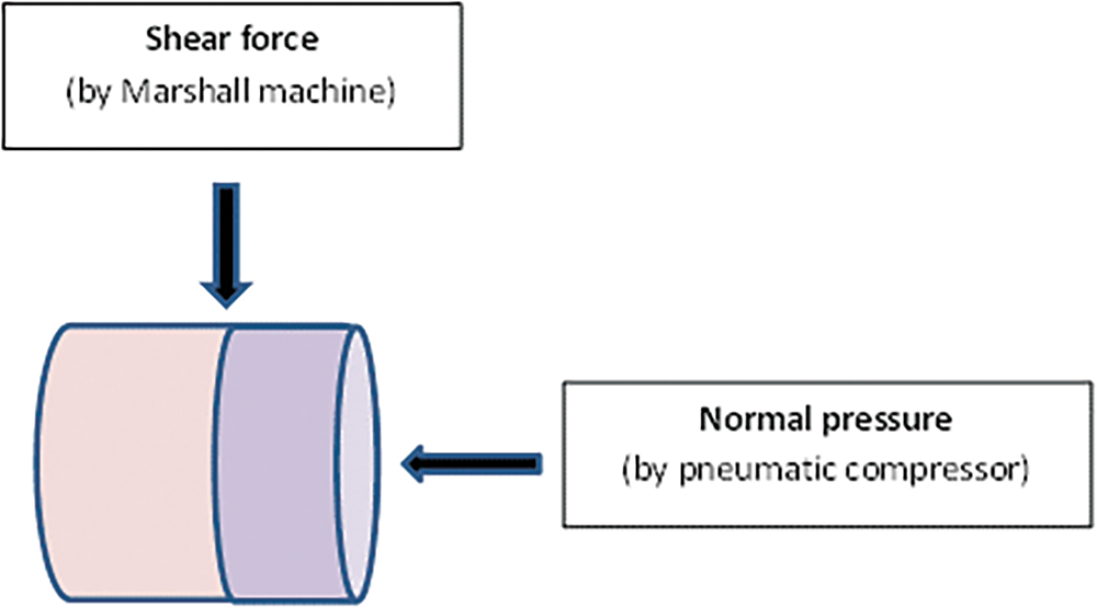
Figure 1: Shear test mechanism

These parameters of temperature (T), tack coat rate (R), and normal pressure (P) is considered as input variables for building models to determine the output variable (SBS). The selected temperatures of 25°C, 40°C, and 60°C represent the actual operating conditions of flexible pavement structures, corresponding to medium, high, and very high-temperature scenarios. This selection is based on the AASHTO TP 114-15 guidelines, which suggest a standard temperature of 25°C, and the range used in other research studies (20°C–60°C) [12,15,16]. For normal pressure, we selected 0, 0.2, 0.4, and 0.6 MPa, referencing global research, which typically ranges from 0 to 0.8 MPa (10, 12, 15, 51). These pressures reflect realistic conditions that pavement structures might experience. The selected tack coat rates of 0.0, 0.2, 0.5, and 0.8 l/m2 are based on actual construction practices in Vietnam, where 0.5 l/m2 is commonly used, and aligned with international research findings (0–0.8 l/m2) (7, 16, 52–54). These parameter selections ensure our study accurately reflects real-world conditions and adheres to established experimental criteria.

Table 3 shows statistical analyses of the inputs and output. In addition, a histogram of each input and output parameter is shown in Fig. 2. Correlation plots are crucial as they visually represent the relationships between different variables. For input-input correlations, these plots help identify any multi-collinearity issues where two or more input variables are highly correlated, potentially affecting the model’s performance. For input-output correlations, these plots illustrate the strength and nature of the relationship between each input variable and the output variable, providing insights into which variables have the most significant impact on the model’s predictions. The vertical axis of these plots represents the occurrence frequency (number of samples), while the horizontal axis represents the variable’s value. The height of the columns indicates how frequently each value occurs, helping to understand the distribution of the variable values and their relationships. Analysis of the distribution of values of 240 samples revealed that the mechanical parameters varied across a wide range of values. Temperature had the largest standard deviation, while normal pressure had the smallest.

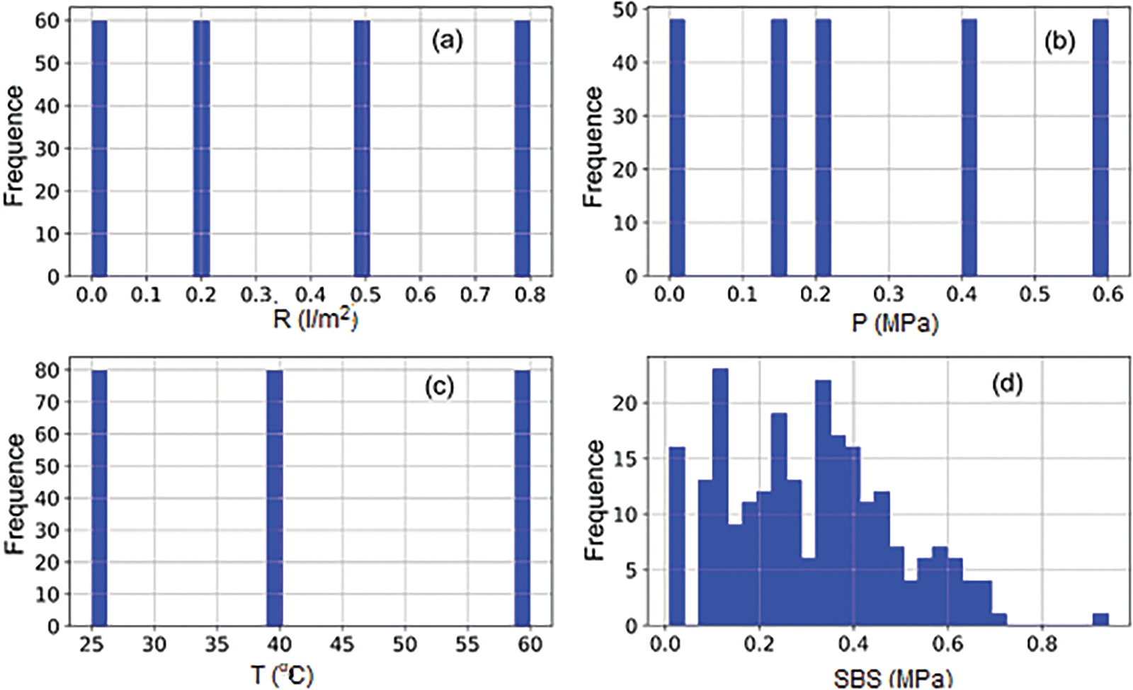
Figure 2: Histogram of the input and output parameters: (a) R, (b) P, (c) T, (d) SBS

The evaluation of the input variable spatial domain is an important step for the models to predict more accurately and simulate faster. The correlation between input-input and input-output is an important basis for choosing suitable input parameters for the forecasting model. Therefore, a correlation matrix between the parameters was analyzed and illustrated in Fig. 3. Positive correlations are indicated by blue squares, whereas negative correlations are indicated by yellow squares. At the same time, the color intensity shows the correlation level. To limit the impact of extraneous factors on the prediction model, pairs of features having a high correlation can be eliminated. Accordingly, pairs of attributes with a correlation greater than 0.75 or less than −0.75 are considered highly correlated attribute pairs and should be carefully considered. Initial analysis indicates that all input factors have a low to moderate correlation with each other and are therefore considered independent variables. The predicted SBS, which is based on these inputs, is the dependent variable.

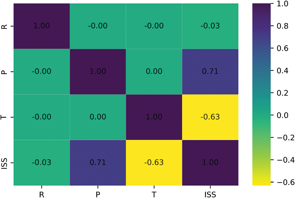
Figure 3: Correlation matrix analysis of input variables

2.2 Methods Used

This study adhered to the proposed methodology, which is structured around the following key steps (Fig. 4):

1.    Data Preparation: The collected experimental results were divided into two subsets: a training dataset (70%) used to train the models and a testing dataset (30%) used to evaluate their performance.

2.    Model Training: Cross-validation and parameter optimization using Grid Search CV were applied to build three models: KNN, ET, and LGBM.

3.    Model Validation: The effectiveness of the models was evaluated and compared by using statistical indicators, namely RMSE, MAE, and R2. The best model was then selected and its learning curve results were evaluated.

4.    Analysing Sensitivity: SHAP was applied to assess the impact of inputs on SBS.

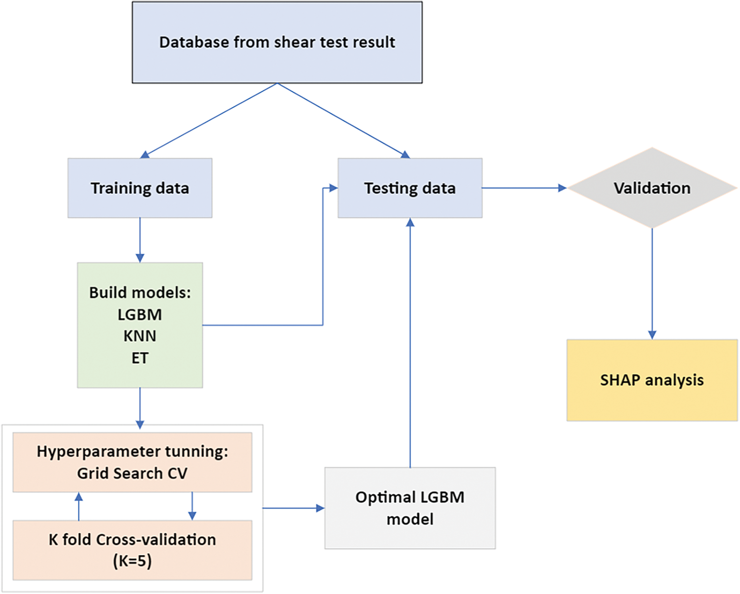
Figure 4: Methodological flow chart

2.2.1 K-Nearest Neighbors (KNN)

KNN is an algorithm used in ML with supervised learning to make decisions or predict the future. KNN uses mathematical formulas to select the K closest elements from the training dataset to make decisions. True to the algorithm’s name, labeling or predicting the outcome of an example is based on the most recent learning examples [46].

After loading the database, the KNN algorithm calibrates the value of K to determine the desired number of neighbors. For each data point, the following steps are performed: computing the distance between the query sample and the current sample, adding this distance to an organized collection, sorting the dataset in ascending order of distance, selecting the first K items from the sorted collection, obtaining the labels for the K chosen items, and finally returning the mean of the K labels [38,47].

KNN is an essential and transparent algorithm that is also highly successful due to its non-parametric nature (Fig. 5). It requires no inferences regarding the data distribution. Obviously, the choice of K will probably affect the algorithm’s accuracy. The accuracy will increase significantly with a large enough training data set and the ability to produce a reasonably large number of K [49].

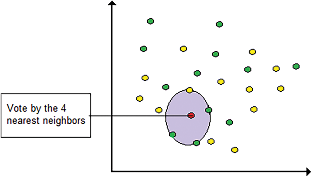
Figure 5: Illustration of KNN algorithm

2.2.2 Extra Trees (ET)

ET is a technique similar to Random Forest classification, aggregating the results of multiple uncorrelated decision trees [50]. While sub-trees can sometimes outperform Random Forests, ET employs a simpler method to create decision trees for the ensemble. Typically, decision trees exhibit high variance, whereas Random Forests tend to have medium variance [39,51]. When model accuracy is prioritized over generalization, ET often produces low variance. Additionally, ET is relatively easy to implement, requiring only a few key hyperparameters, with straightforward heuristics for tuning them [52]. The ET approach generates many unpruned decision trees using the training data. Predictions are made by averaging the results from these decision trees (Fig. 6).

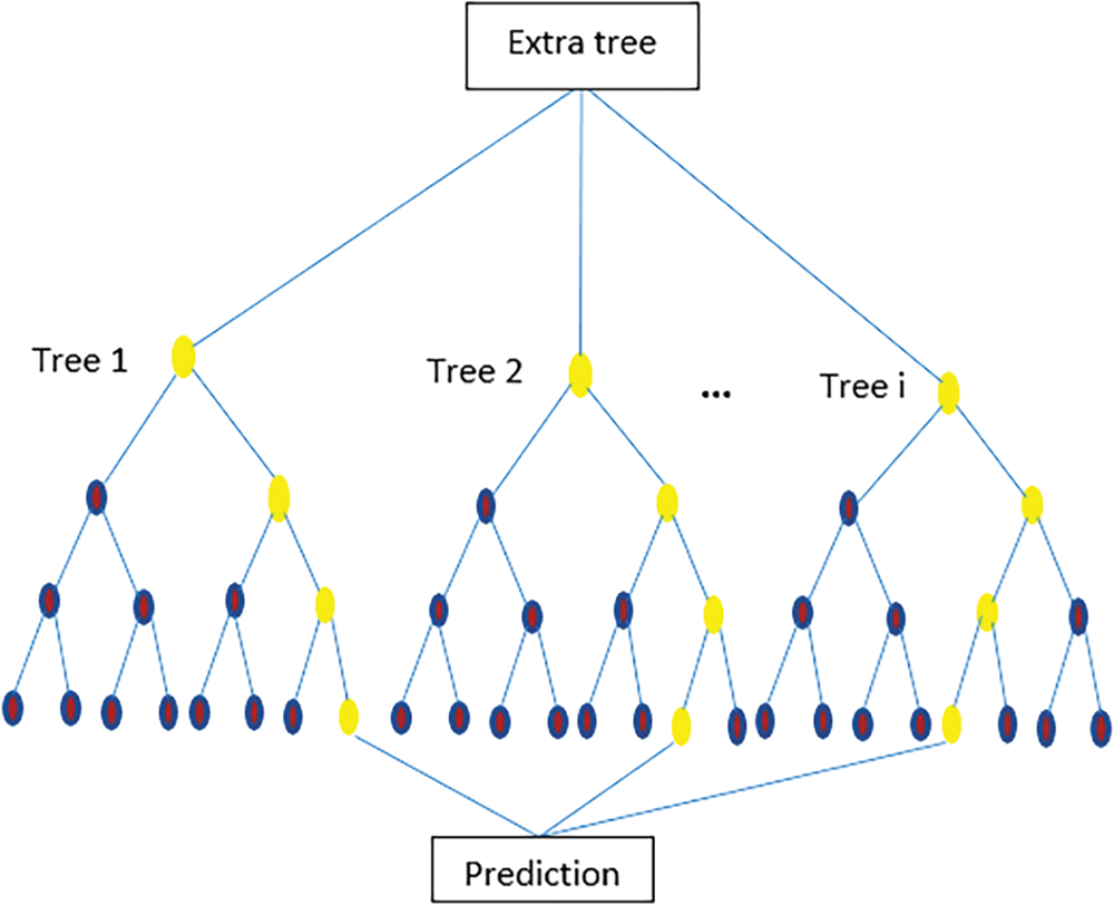
Figure 6: Illustration of ET algorithm

2.2.3 Light Gradient Boosted Machine (LGBM)

LGBM is an open-source gradient-boosting library based on decision tree algorithms. It employs a histogram-based method that splits continuous variables into different groups rather than sorting individual controls [53]. Additionally, LGBM uses a leaf-wise tree growth approach (Fig. 7) instead of the level-wise method used by most other decision tree-based algorithms, which helps improve model efficiency, reduce memory usage, and enhance computation time [29]. This makes LGBM particularly well-suited for larger datasets, where other methods may struggle with performance. Despite handling larger data sizes, LGBM maintains or improves model performance while significantly reducing runtime [54].

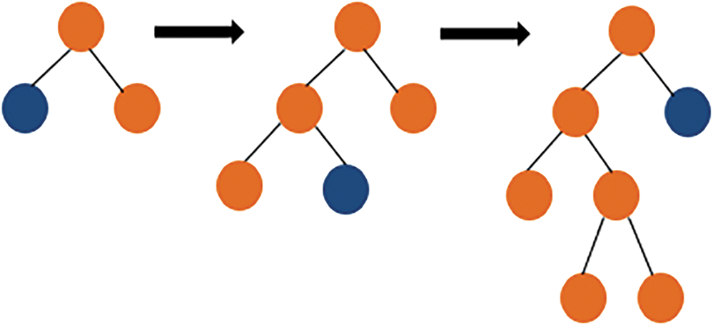
Figure 7: Illustration of leaf-wise tree growth

2.2.4 Grid Search CV Optimization Technique

Most parameters in an ML model are learned directly from the data, but some, known as hyperparameters, cannot be learned in this way. Regardless of the model’s complexity or learning rate, these hyperparameters significantly affect the model’s performance. Finding the optimal combination of hyperparameters is challenging, as the model may have numerous hyperparameters that interact in complex ways [55]. Cross-validation is typically employed in a cyclic process to identify the best parameter set. Once the optimal combination is found, the process is repeated on all available data (without cross-validation) to generate a final model with the best settings [56,57].

The Grid Search (Fig. 8) algorithm is a commonly used approach for hyperparameter tuning, involving testing all possible combinations from a predefined grid of hyperparameters. This method allows for identifying the best parameters from a list of given options through exhaustive searching [55,57].

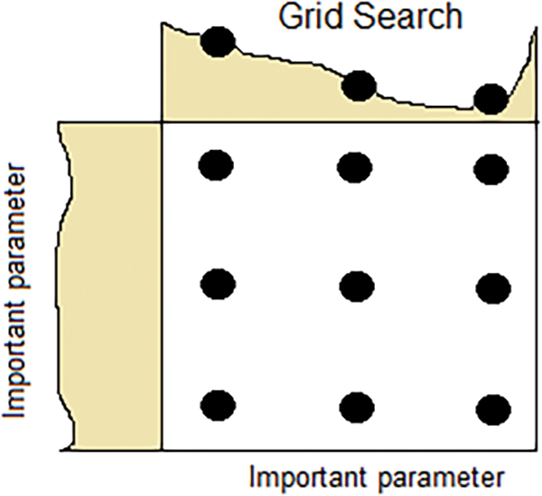
Figure 8: Illustration of Grid Search CV algorithm

2.2.5 Validation Indicators

Statistical indicators

To evaluate the performance of ML models, three statistical measures were applied: Root Mean Square Error (RMSE), Mean Absolute Error (MAE), and Coefficient of Determination (R2). RMSE represents the standard deviation of the model’s prediction errors, while MAE calculates the average of the absolute errors. R2 is a metric that describes the relationship between a pair of variables and takes a value from 0 to 1, with a larger value reflecting the greater accuracy of the model. These statistical measures have been widely used in previous studies [28–31].

Cross-validation

Cross-validation is a technique of subdividing datasets to verify the model’s performance on separate parts (Fig. 9). This technique is easy to understand and implement. It provides more reliable estimates than other methods [58]. The important element in the method is that k represents the number of groups into which the data set shall be separated. The procedure typically entails the subsequent phases: Randomly circulate the data set and split it into k fold. With each part: The present fold assesses the model’s effectiveness; the remaining folds serve for model training and evaluation [30,59,60].

Figure 9: Illustration of Cross-validation technique

It is critical to remember that each sample is allocated a certain fold and must remain in that fold for the duration of the process. Data preparation is only done on the divided training set, not on the entire dataset. Typically, the aggregated result is the mean of the evaluations. Additionally, including variance and standard deviation information in the aggregated findings is used in practice [61].

Learning curve

The learning curve, initially used to describe the relationship between performance and training in machine learning, was first introduced in 1885 by H. Ebbinghaus [62]. A graph illustrates a model’s performance over time [63]. It also describes the loss of the training and validation datasets. The learning curve graphs provide information on the model’s learning dynamics, such as whether it is learning well under-fitting or overfitting with the training dataset. Learning curves can be used to compare alternative methods, choose model parameters during design, do hyperparameter tuning to optimize convergence and figure out the required data size [53].

SHAP analysis

SHAP is a method for calculating each attribute’s contribution to an objective variable’s value [39]. The goal is to conceptualize each feature as a “player,” with the dataset representing the “team.” Each player (feature) contributes to the team’s overall performance (the target variable). The aggregate of these contributions determines the final prediction or value. Importantly, the influence of a feature depends on the full set of features in the dataset, not just on the individual feature alone [41,64].

SHAP employs combinatorial mathematics to calculate the impact of every feature on the objective variable (referred to as the SHAP value). It works by considering all possible feature combinations and retraining the model accordingly. The average absolute value of a feature’s SHAP value can be used to assess its overall importance. One of SHAP’s key advantages is that it is model-agnostic, meaning it can be applied to any model without being constrained by the specific choice of algorithm. This makes it ideal for explaining models that do not inherently provide feature importance assessments [64,65].

3  Results and Discussions

3.1 Model Validation and Comparison

Building ML models involves determining the optimal values for the model’s hyperparameters. This study used a five-fold cross-validation approach to split the training dataset and evaluate the models’ performance. The Grid Search CV method was employed to find optimal hyperparameters and fit the predictive model features. It makes finding hyperparameters that result in optimal model estimation accuracy easier. The estimator n_neighbors, which represents the number of nearest neighbors in the model and the number of weak learners, are important hyperparameters. In addition, parameters such as the weights, maximum depth, and learning rate can substantially affect the model’s predictive capacity. The hyperparameters considered in the Grid Search CV are listed in Table 4.

The results of the performance evaluation for the models are presented in Table 5. The results indicate that all three models achieved high accuracy (R2 > 0.91) in both the training and testing phases. The use of 5-fold cross-validation and the Grid Search CV method contributed to the high accuracy of the SBS prediction models. The KNN and ET models demonstrated slightly higher training accuracy (R2 = 0.974 and 0.977, respectively) than the LGBM model (R2 = 0.965). However, they exhibited significantly lower testing accuracy (R2 = 0.914 and 0.921, respectively) than LGBM (R2 = 0.961).

Notably, the verification data (30% of the dataset) was not used in the model-building process. The hyperparameters for each model were selected based solely on the training and testing datasets. The LGBM model exhibited the most stable performance and highest accuracy on the test dataset, with an R2 of 0.961, RMSE of 0.35, and MAE of 0.22. After conducting five-fold cross-validation and Grid Search CV, the LGBM model emerged as the most accurate. Therefore, we selected this model to present our forecast results.

The regression approach shows the correlation between the SBS values predicted by the LGBM model and the actual values from experiments for the training and testing datasets (Fig. 10). The horizontal axis represents the SBS values from the actual tests. In contrast, the vertical axis shows the predictions made by the model. The LGBM model’s predictions for the training dataset (Fig. 10a) and the testing dataset (Fig. 10b) are very close to the experimental results. These findings demonstrate that the LGBM model provides reliable prediction results. The correlation between the LGBM model and the actual training and testing datasets outcomes is very high, with R2 values of 0.965 and 0.961, respectively. The model’s performance is stable across both phases, as the R2 values are nearly identical, highlighting the LGBM model’s strong predictive capability.

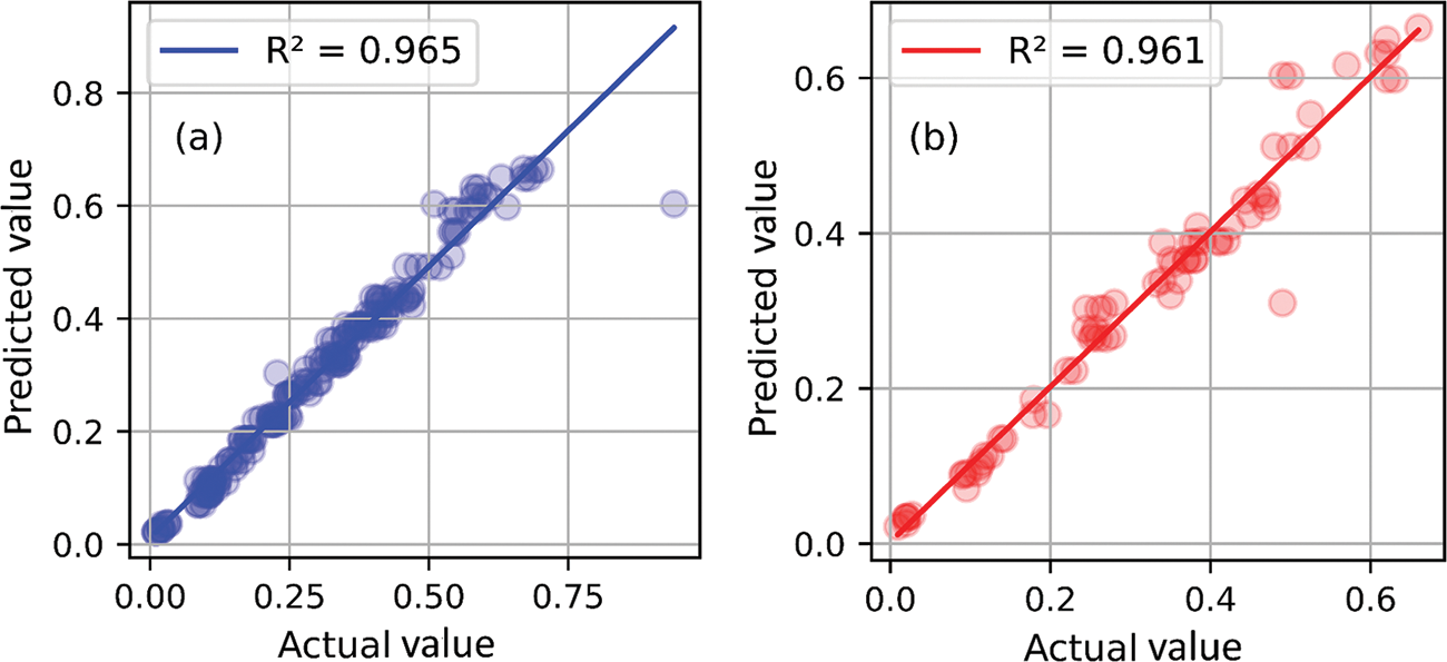
Figure 10: R2 values with (a) training, (b) testing dataset for LGBM model

The learning curve for the LGBM model is shown in Fig. 11. The vertical axis represents the learning score, while the horizontal axis indicates the size of the training dataset. Solid lines represent the mean scores for the training set (blue line) and cross-validation (red line). The results indicate that the training and cross-validation scores follow similar trends. Both scores increase gradually as the training data size grows, eventually stabilizing. When the training dataset size is less than 47, underfitting is observed. However, the model fits well without overfitting when the training dataset size ranges from 120 to 148.

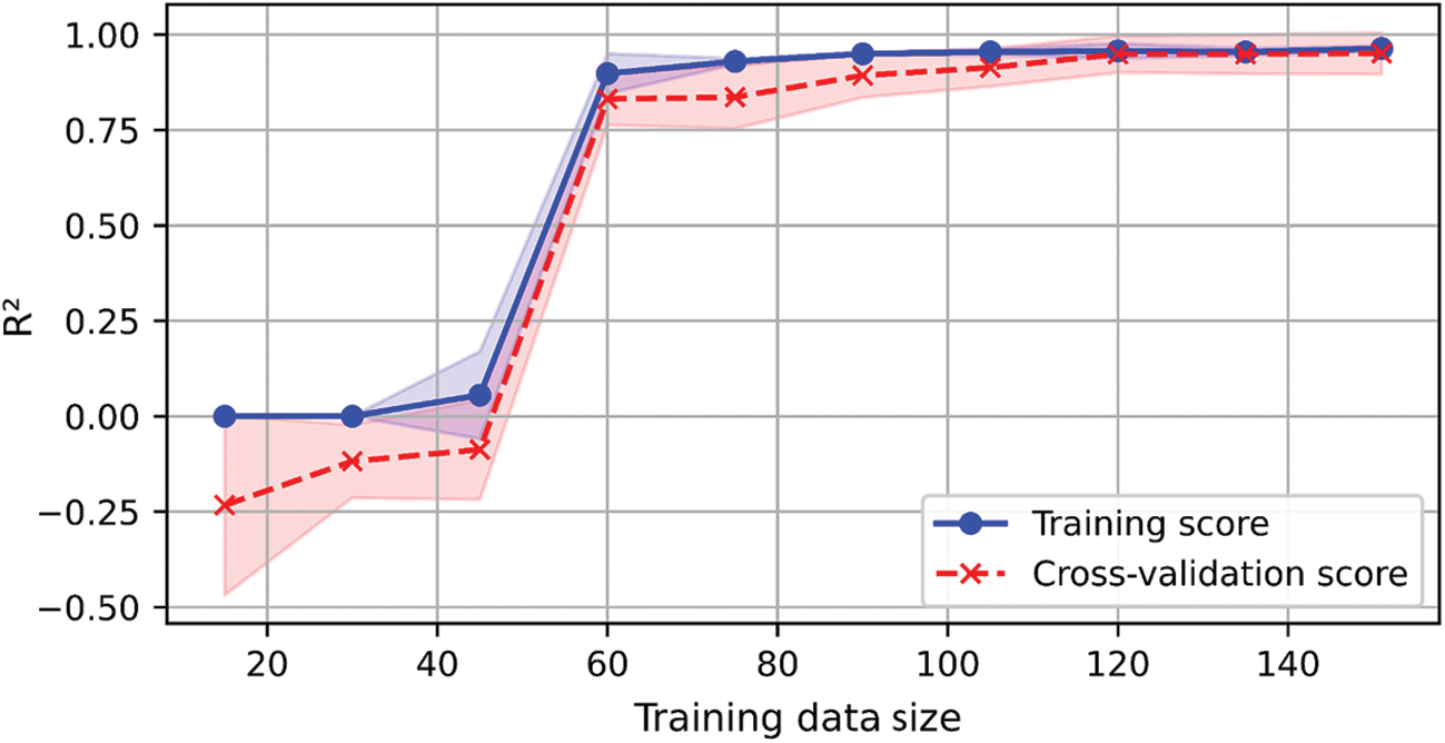
Figure 11: Learning curve analysis of LGBM

To provide a more detailed comparison, the simulated RMSE error distribution graphs of the LGBM model for the training, validation, and verification datasets are shown in Fig. 12. In both cases, the errors are densely concentrated near the 0 kN point. Furthermore, the error distributions show that nearly 95% of the errors fall within a relatively narrow range of around 0 kN, indicating the model’s strong ability to simulate SBS accurately. Only a few large errors (exceeding 0.1 and 0.2 MPa) were observed, but these do not significantly impact the model’s generalizability. Overall, LGBM proves to be an efficient algorithm for predicting SBS.

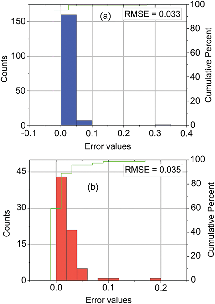
Figure 12: RMSE values with (a) training, (b) testing for LGBM model

LGBM has demonstrated its robustness and superior performance in various forecasting tasks across different fields. For example, Hartanto et al. [66] compared LGBM with other boosting algorithms, such as XGBoost, AdaBoost, and CatBoost, for forecasting stock price and concluded that LGBM provided higher accuracy. Stawiski et al. [67] reported that LGBM achieved better efficiency than RF in predicting quantitative structure-activity relationships with faster computation speed.

LGBM’s high accuracy and superior efficiency can be attributed to its fast training speed, low memory usage, GPU support, parallel learning capabilities, and ability to handle large-scale data [68]. However, it is important to note that LGBM may not always be the best choice for every scenario. For instance, Hindarto [69] found that the Gradient Boosting Machine (R2 = 0.82) slightly outperformed LGBM (R2 = 0.81) in predicting landslide risk. Therefore, while LGBM is a powerful algorithm, it is crucial to evaluate and select the most appropriate model based on the specific dataset and problem at hand.

LGBM is recognized as a powerful and efficient algorithm due to its memory efficiency and scalability, making it particularly well-suited for large, high-dimensional, and imbalanced datasets [70,71]. One of its key features is the use of a histogram-based approach for building decision trees. This method leverages Gradient-based One-Side Sampling (GOSS) to randomly select a portion of the data for each tree split, improving computational efficiency and helping to mitigate overfitting, especially in datasets with many attributes [72]. Another significant characteristic of LGBM is its leaf-wise tree growth strategy, which identifies the optimal split point within a leaf in contrast to traditional level-wise methods. This approach allows LGBM to achieve higher accuracy but can increase the risk of overfitting, particularly as the number of trees grows. Additionally, LGBM effectively handles imbalanced datasets by assigning different weights to various classes, making it well-suited for sparse data and datasets with missing values [71,72].

However, LGBM is not without its challenges. Like other tree-based algorithms, it is prone to overfitting, especially when a large number of trees are used. Moreover, the numerous hyperparameters requiring tuning make LGBM more complex than some other machine learning models [71]. For this study, we employed Grid Search CV for hyperparameter tuning, effectively addressing LGBM’s potential shortcomings and maximizing its performance in SBS prediction despite the limitations posed by the relatively small dataset.

3.2 Importance of the Input Parameters Used in the Modelling

The SHAP analysis results are described in Fig. 13. The dot plot shows the SHAP value density distribution for factors important in predicting SBS. A high SHAP score suggests that this characteristic indicates that the subject has an SBS. Certain representative SHAP interpretations are described by a unique dot per row that characterizes each sample. The feature’s SHAP value determines the position of the dot and the stacked dots along each row to show the density. Color is used in a graph to display the initial value of a feature.

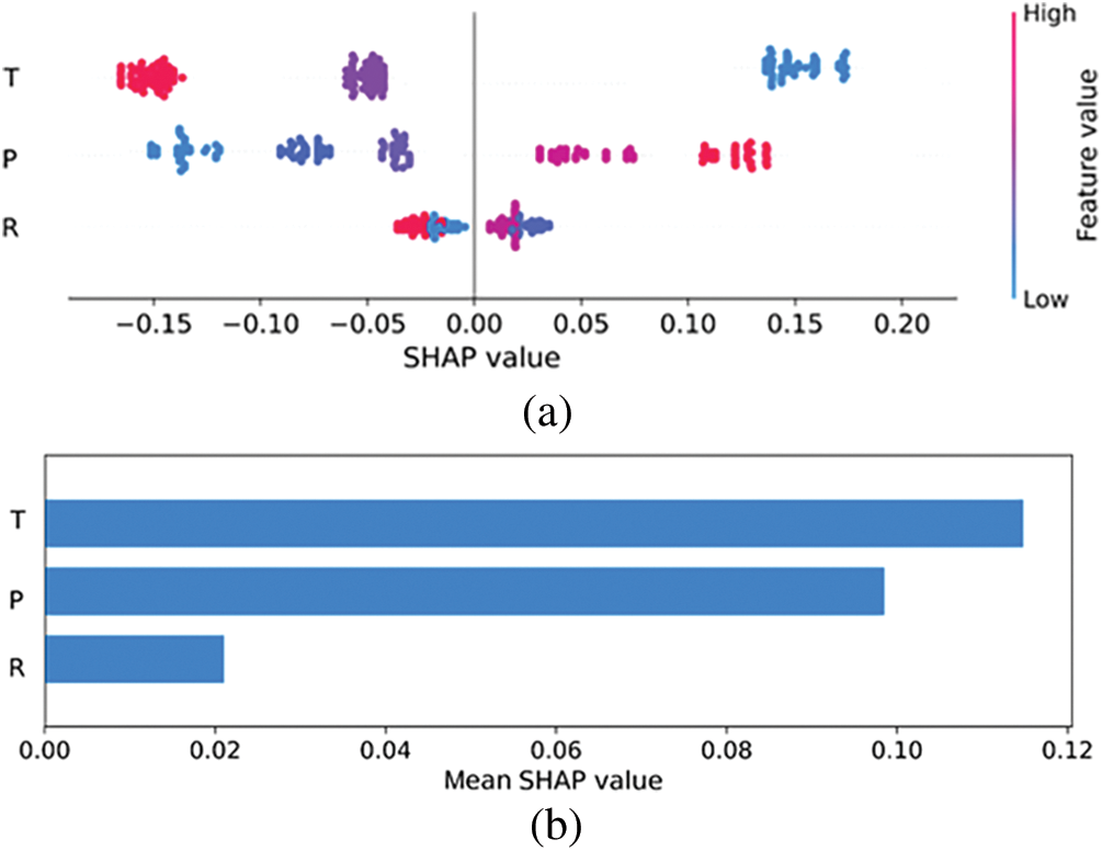
Figure 13: Analysis of SHAP values of input parameters used in the LGBM model (Note: temperature (T), tack coat rate (R), normal pressure (P))

The bar graph depicts the overall importance of the attribute as expressed by the subject’s absolute SHAP value for the attribute across all samples. This graph depicts the three most critical characteristics for predicting SBS. This is represented as the mean of the absolute value of the SHAP score for that specific attribute across all subjects. A higher SHAP value suggests that this attribute influences model predictions.

The SHAP analysis results indicate that, among the three factors examined, temperature is the most influential factor on SBS, while the tack coat rate has the least impact. This finding aligns with results from previous studies [1,6,12,73]. Temperature is considered the most influential factor on SBS between two layers of asphalt concrete because the mechanical properties of bituminous materials are highly sensitive to temperature variations. At low temperatures, the material exhibits elasticity, while at high temperatures, it exhibits viscoelasticity. Several studies have shown that SBS can decrease by 40%–90% when the temperature increases from 10°C to 60°C [16,23,74–76]. In addition, the SHAP analysis reveals that normal pressure also significantly affects SBS. Canestrari et al. [15], Uzan et al. [73] and West et al. [12] noted that normal pressure is proportional to SBS due to the substantial increase in friction at the interface between asphalt concrete layers, as described by Mohr-Coulomb theory.

On the other hand, Fig. 13 shows that while the tack coat rate does influence SBS, its effect is less significant than that of temperature and normal pressure. Previous research by Mohamad et al. [16], Chen et al. [77], Zhang et al. [76], also found that both insufficient and excessive tack coat application can reduce SBS. A lack of tack coat leads to poor bonding, while an excess can cause slippage at the interface. However, these studies agree that tack coat rate is only one factor influencing SBS, with temperature remaining the most critical determinant.

Based on the analysis of key variables such as temperature, pressure, and tack coat rate, we offer practical recommendations to enhance the applicability of the study’s findings. To achieve optimal SBS, pavement structures should generally operate in low to medium temperature environments with appropriate loads, and the tack coat layer should be applied at an optimal rate. However, modifying these factors may be challenging since the road’s design capacity often dictates operating temperature and vehicle load. Therefore, we propose indirect solutions, such as using specialized tack coat materials in high-temperature regions and implementing measures to control vehicle loads to prevent overloading. Additionally, ensuring uniform application of the tack coat is crucial; even if the tack coat ratio is correctly designed, uneven distribution can significantly reduce SBS performance.

Our study employed a moderate sample size of 240 data sets, which has been validated to ensure the reliability of the results. While we focused on three key variables—temperature, tack coat rate, and normal pressure—future research will include additional factors, such as separation time, types of tack coat materials, and surface conditions. We are also exploring data augmentation techniques and models suited for small sample learning to improve prediction accuracy further. These efforts will address current limitations and contribute to a more comprehensive and generalizable understanding of SBS.

4  Conclusion

SBS between double-layer asphalt concrete is critical for designing flexible pavement structures and assessing pavement quality. Traditionally, determining SBS requires complex and costly shear tests. This study explored using three machine learning algorithms—KNN, ET, and LGBM—optimized through Grid Search and cross-validation to predict SBS. Utilizing a dataset of 240 experimental results, input variables including temperature, normal pressure, and tack coat rate, the LGBM model demonstrated the highest performance, achieving an R2 value of 0.961.

SHAP analysis revealed that temperature is the most significant factor influencing SBS, validating its importance in pavement design. The findings suggest that machine learning models, particularly LGBM, provide an effective and efficient alternative for predicting SBS, potentially reducing reliance on costly traditional methods.

As the development of predictive models is an ongoing process, future research should focus on applying more advanced models to larger and more diverse datasets. Additionally, incorporating extra variables such as humidity, tack coat type, and interface conditions could further enhance the precision and applicability of SBS predictions. The proposed machine learning models offer a rapid and accurate approach to predicting SBS between asphalt concrete layers, providing valuable insights for flexible pavement design.

Acknowledgement: This work was supported by the University of Transport Technology, Thanh Xuan, Hanoi, Vietnam (UTT).

Funding Statement: This research was funded by the University of Transport Technology under grant number DTTD2022-12.

Author Contributions: All authors contributed to the study conception and design. Material preparation, data collection and analysis were performed by Quynh-Anh Thi Bui, Dam Duc Nguyen, Hiep Van Le, Indra Prakash, Binh Thai Pham. The first draft of the manuscript was written by Quynh-Anh Thi Bui. All authors reviewed the results and approved the final version of the manuscript.

Availability of Data and Materials: The data used to generate the numerical results included in this paper are available from the corresponding author on request.

Ethics Approval: Not applicable.

Conflicts of Interest: The authors declare no conflicts of interest to report regarding the present study.

References

1. Nguyen NL, Dao VD, Nguyen ML, Pham DH. Investigation of bond between asphalt layers in flexible pavement. In: 8th RILEM International Conference on Mechanisms of Cracking and Debonding in Pavements, 2016; Nantes, France, Springer; p. 519–25. doi:10.1007/978-94-024-0867-6_73. [Google Scholar] [CrossRef]

2. 22TCN-211. Design flexible pavement structure. 2006. Available from: https://chinhphu.vn/default.aspx?pageid=27160&docid=19321. [Accessed 2024]. [Google Scholar]

3. Claessen AIM, Edwards JM, Sommer P, Uge P. Asphalt pavement design–the shell method. In: Volume I of proceedings of 4th International Conference on Structural Design of Asphalt Pavements, 1977, January; Ann Arbor, Michigan, August 22–26, 1977. [Google Scholar]

4. Kruntcheva MR, Collop AC, Thom NH. Properties of asphalt concrete layer interfaces. J Mater Civ Eng. 2006;18:467–71. doi:10.1061/(asce)0899-1561(2006)18:3(467). [Google Scholar] [CrossRef]

5. Leutner R. Investigation of the adhesion of bituminous pavements. Bitumen. 1979;3:84–91. [Google Scholar]

6. Collop AC, Thom NH. The importance of bond between pavement layers. Final Summary Report to EPSRC, NCPE, Nottingham; 2002. [Google Scholar]

7. Bui Q-AT. Effect of tack coat application rate and temperature on interlayer cohesion and friction of double-layer asphalt samples. In: CIGOS 2021, Emerging Technologies and Applications for Green Infrastructure. Singapore: Springer Nature; 2022. p. 595–606. doi:10.1007/978-981-16-7160-9_60. [Google Scholar] [CrossRef]

8. Bui Q-AT, Lee JS, Kieu TQ. Evaluation of shear bond for double-layer asphalt concrete samples based on shear test. J Sci Transp Technol. 2023;3(2):11–8. doi:10.58845/jstt.utt.2023.en.3.2.11-18. [Google Scholar] [CrossRef]

9. Yang K, Li R. Characterization of bonding property in asphalt pavement interlayer: a review. J Traf Transport Eng (English Edition). 2021;8:374–87. doi:10.1016/j.jtte.2020.10.005. [Google Scholar] [CrossRef]

10. Canestrari F, Ferrotti G, Partl MN, Santagata E. Advanced testing and characterization of interlayer shear resistance. Transp Res Rec. 2005;1929:69–78. doi:10.3141/1929-09. [Google Scholar] [CrossRef]

11. Zofka A, Maliszewski M, Bernier A, Josen R, Vaitkus A, Kleizienė R. Advanced shear tester for evaluation of asphalt concrete under constant normal stiffness conditions. Road Mater Pavement Des. 2015 May 25;16(sup1):187–210. doi:10.1080/14680629.2015.1029690. [Google Scholar] [CrossRef]

12. West RC, Zhang J, Moore J. Evaluation of bond strength between pavement layers. NCAT Report 05–08. Auburn University. National Center for Asphalt Technology; 2005. [Google Scholar]

13. Hakim BA. The importance of good bond between bituminous layers. In: Ninth International Conference on Asphalt Pavements International Society for Asphalt Pavements, 2002; Copenhagen, Denmark. [Google Scholar]

14. Hachiya Y, Umeno S, Sato K. Effect of tack coat on bonding characteristics at interface between asphalt concrete layers. Doboku Gakkai Ronbunshu. 1997;1997(571):199–209. doi:10.2208/jscej.1997.571_199. [Google Scholar] [CrossRef]

15. Canestrari F, Ferrotti G, Lu X, Millien A, Partl MN, Petit C, et al. Mechanical testing of interlayer bonding in asphalt pavements. In: Advances in interlaboratory testing and evaluation of bituminous materials. Springer, NY, USA, 2013. p. 303–60. doi:10.1007/978-94-007-5104-0_6. [Google Scholar] [CrossRef]

16. Mohammad LN, Hassan M, Patel N. Effects of shear bond characteristics of tack coats on pavement performance at the interface. Transp Res Rec. 2011;2209(1):1–8. doi:10.3141/2209-01. [Google Scholar] [CrossRef]

17. Ai C, Rahman A, Song J, Gao X, Lu Y. Characterization of interface bonding in asphalt pavement layers based on direct shear tests with vertical loading. J Mater Civ Eng. 2017 Sep 1;29(9):04017102. doi:10.1061/(ASCE)MT.1943-5533.0001952. [Google Scholar] [CrossRef]

18. You L, Yan K, Liu N. Assessing artificial neural network performance for predicting interlayer conditions and layer modulus of multi-layered flexible pavement. Front Struct Civil Eng. 2020;14(2):487–500. doi:10.1007/s11709-020-0609-4. [Google Scholar] [CrossRef]

19. Romanoschi SA, Metcalf JB. Characterization of asphalt concrete layer interfaces. Transp Res Rec. 2001;1778(1):132–9. doi:10.3141/1778-16. [Google Scholar] [CrossRef]

20. Lushinga N, Xin J. Effect of horizontal shear load on pavement performance. In: International Proceedings of Chemical, Biological and Environmental Engineering, 2015; Singapore; p. 80. [Google Scholar]

21. Mattos JR, Núñez WP, Ceratti JA, Zíngano A, Fedrigo W. Shear strength of hot-mix asphalt and its relation to near-surface pavement failure–a case study in Southern Brazil. In: E & E Congress, 2016 Jun; Prague, Czech Republic. doi:10.14311/ee.2016.240. [Google Scholar] [CrossRef]

22. Kim H, Arraigada M, Raab C, Partl MN. Numerical and experimental analysis for the interlayer behavior of double-layered asphalt pavement specimens. J Mater Civ Eng. 2011;23(1):12–20. doi:10.1061/(ASCE)MT.1943-5533.0000003. [Google Scholar] [CrossRef]

23. Chun S, Kim K, Greene J, Choubane B. Evaluation of interlayer bonding condition on structural response characteristics of asphalt pavement using finite element analysis and full-scale field tests. Constr Build Mater. 2015;96(1–2):307–18. doi:10.1016/j.conbuildmat.2015.08.031. [Google Scholar] [CrossRef]

24. Pham BT, Tien Bui D, Dholakia MB, Prakash I, Pham HV. A comparative study of least square support vector machines and multiclass alternating decision trees for spatial prediction of rainfall-induced landslides in a tropical cyclones area. Geotech Geol Eng. 2016 Dec;34(6):1807–24. doi:10.1007/s10706-016-9990-0. [Google Scholar] [CrossRef]

25. Zhang Y, Yang H, Lin J, Xu P, Liu J, Zeng Y, et al. Susceptibility assessment of earthquake-induced landslide by using back-propagation neural network in the Southwest mountainous area of China. Bull Eng Geol Environ. 2024 May;83(5):187. doi:10.1007/s10064-024-03687-w. [Google Scholar] [CrossRef]

26. Solaimani K, Darvishi S, Shokrian F. Assessment of machine learning algorithms and new hybrid multi-criteria analysis for flood hazard and mapping. Environ Sci Pollut Res. 2024;31(22):32950–71. doi:10.1007/s11356-024-33288-9. [Google Scholar] [CrossRef]

27. He R, Zhang W, Dou J, Jiang N, Xiao H, Zhou J. Application of artificial intelligence in three aspects of landslide risk assessment: a comprehensive review. Rock Mechan Bullet. 2024 Jul 6;3(4):100144. doi:10.1016/j.rockmb.2024.100144. [Google Scholar] [CrossRef]

28. Mai H-VT, Nguyen MH, Trinh SH, Ly H-B. Toward improved prediction of recycled brick aggregate concrete compressive strength by designing ensemble machine learning models. Constr Build Mater. 2023;369:130613. doi:10.1016/j.conbuildmat.2023.130613. [Google Scholar] [CrossRef]

29. Thi Mai H-V, Hoang Trinh S, Ly H-B. Enhancing Compressive strength prediction of Roller Compacted concrete using Machine learning techniques. Measurement. 2023;218(1):113196. doi:10.1016/j.measurement.2023.113196. [Google Scholar] [CrossRef]

30. Nguyen T-A, Trinh SH, Nguyen MH, Ly H-B. Novel ensemble approach to predict the ultimate axial load of CFST columns with different cross-sections. Structures. 2023;47:1–14. doi:10.1016/j.istruc.2022.11.047. [Google Scholar] [CrossRef]

31. Hadzima-Nyarko M, Trinh SH. Prediction of compressive strength of concrete at high heating conditions by using artificial neural network-based Bayesian regularization. J Sci Transp Technol. 2022;2(1):9–21. doi:10.58845/jstt.utt.2022.en.2.1.9-21. [Google Scholar] [CrossRef]

32. Ceylan H, Guclu A, Tutumluer E, Thompson MR. Backcalculation of full-depth asphalt pavement layer moduli considering nonlinear stress-dependent subgrade behavior. Int J Pavement Eng. 2005;6(3):171–82. doi:10.1080/10298430500150981. [Google Scholar] [CrossRef]

33. Meier RW, Alexander DR, Freeman RB. Using artificial neural networks as a forward approach to backcalculation. Transp Res Rec. 1997;1570(1):126–33. doi:10.3141/1570-15. [Google Scholar] [CrossRef]

34. Tapkın S, Çevik A, Özcan Ş. Utilising neural networks and closed form solutions to determine static creep behaviour and optimal polypropylene amount in bituminous mixtures. Mater Res. 2012;15(6):865–83. doi:10.1590/S1516-14392012005000117. [Google Scholar] [CrossRef]

35. Raab C, Partl MN. Utilisation of artificial neural network for the analysis of interlayer shear properties. Balt J Road Bridge Eng. 2013;8:107–16. doi:10.3846/bjrbe.2013.14. [Google Scholar] [CrossRef]

36. Van Dao D, Bui QA, Nguyen DD, Prakash I, Trinh SH, Pham BT. Prediction of interlayer shear strength of double-layer asphalt using novel hybrid artificial intelligence models of ANFIS and metaheuristic optimizations. Constr Build Mater. 2022 Mar 14;323:126595. doi:10.1016/j.conbuildmat.2022.126595. [Google Scholar] [CrossRef]

37. AL-Jarazi R, Rahman A, Ai C, Al-Huda Z, Ariouat H. Development of prediction models for interlayer shear strength in asphalt pavement using machine learning and SHAP techniques. Road Mater Pavement Des. 2024;11:1–9. doi:10.1080/14680629.2023.2276412. [Google Scholar] [CrossRef]

38. Peterson LE. K-nearest neighbor. Scholarpedia. 2009;4:1883. [Google Scholar]

39. John V, Liu Z, Guo C, Mita S, Kidono K. Real-time lane estimation using deep features and extra trees regression. In: Image and Video Technology, Auckland, New Zealand: Springer International Publishing; 2016. vol. 7, pp. 721–33. [Google Scholar]

40. Bugaj M, Wrobel K, Iwaniec J. Model explainability using SHAP values for LightGBM predictions. In: 2021 IEEE XVIIth International Conference on the Perspective Technologies and Methods in MEMS Design (MEMSTECH), 2021; Polyana (ZakarpattyaUkraine; p. 102–6. doi:10.1109/memstech53091.2021.9468078. [Google Scholar] [CrossRef]

41. Wang D, Thunéll S, Lindberg U, Jiang L, Trygg J, Tysklind M. Towards better process management in wastewater treatment plants: process analytics based on SHAP values for tree-based machine learning methods. J Environ Manag. 2022 Jan 1;301:113941. [Google Scholar]

42. TCVN-7493. Bitumen—specifications. 2005. Available from: https://thuvienphapluat.vn/TCVN/Giao-thong/TCVN-7493-2005-Bitum-Yeu-cau-ky-thuat-907651.aspx. [Accessed 2024]. [Google Scholar]

43. TCVN-8817. Cationic emulsified asphalt. 2011. Available from: https://moc.gov.vn/vn/_layouts/15/NCS.Webpart.MOC/mt_poup/Intrangweb.aspx?IdNews=52731. [Accessed 2024]. [Google Scholar]

44. TCVN-8820. Standard practice for asphalt concrete mix design using marshall method. 2011. Available from: https://thuvienphapluat.vn/chinh-sach-phap-luat-moi/tag?keyword=Ti%c3%aau%20chu%e1%ba%a9n%20Vi%e1%bb%87t%20Nam%20TCVN8820:2011. [Accessed 2024]. [Google Scholar]

45. TCVN-13567. Specification for construction of hot mix asphalt concrete pavement and acceptance. 2023. Available from: https://thuvienphapluat.vn/TCVN/Xay-dung/TCVN-13567-1-2022-Lop-mat-duong-bang-hon-hop-nhua-nong-Phan-1-919459.aspx. [Accessed 2024]. [Google Scholar]

46. Patrick EA, Fischer III FP. A generalized k-nearest neighbor rule. Inf Control. 1970;16:128–52. doi:10.1016/s0019-9958(70)90081-1. [Google Scholar] [CrossRef]

47. Maltamo M, Kangas A. Methods based on k-nearest neighbor regression in the prediction of basal area diameter distribution. Can J For Res. 1998;28:1107–15. doi:10.1139/x98-085. [Google Scholar] [CrossRef]

48. AASHTO-TP114. Standard method of test for determining the interlayer shear strength (ISS) of asphalt pavement layers. 2015. Available from: https://standards.globalspec.com/std/13399734/aashto-tp-114. [Accessed 2024]. [Google Scholar]

49. Nti IK, Nyarko-Boateng O, Aning J. Performance of machine learning algorithms with different K values in K-fold cross-validation. J Inf Technol Comput Sci. 2021;6:61–71. doi:10.5815/ijitcs.2021.06.05. [Google Scholar] [CrossRef]

50. Polamuri SR, Srinivas K, Mohan AK. Stock market prices prediction using random forest and extra tree regression. Int J Recent Technol Eng. 2019;8:1224–8. doi:10.35940/ijrte.c4314.098319. [Google Scholar] [CrossRef]

51. Ahmad MW, Reynolds J, Rezgui Y. Predictive modelling for solar thermal energy systems: a comparison of support vector regression, random forest, extra trees and regression trees. J Clean Prod. 2018;203:810–21. doi:10.1016/j.jclepro.2018.08.207. [Google Scholar] [CrossRef]

52. Domhan T, Springenberg JT, Hutter F. Speeding up automatic hyperparameter optimization of deep neural networks by extrapolation of learning curves. In: Twenty-Fourth International Joint Conference on Artificial Intelligence, 2015; Freiburg, Germany. doi:10.1609/aaai.v29i1.9354. [Google Scholar] [CrossRef]

53. Alabdullah AA, Iqbal M, Zahid M, Khan K, Amin MN, Jalal FE. Prediction of rapid chloride penetration resistance of metakaolin based high strength concrete using light GBM and XGBoost models by incorporating SHAP analysis. Constr Build Mater. 2022 Aug 22;345(3):128296. doi:10.1016/j.conbuildmat.2022.128296. [Google Scholar] [CrossRef]

54. AASHTO-T245. Resistance to plastic flow of bituminous mixture using marshall apparatus. 1997. Available from: https://nazhco.com/wp-content/uploads/2020/06/aashto-t245.pdf. [Accesses 2024]. [Google Scholar]

55. Sun Y, Ding S, Zhang Z, Jia W. An improved grid search algorithm to optimize SVR for prediction. Soft Comput. 2021;25(7):5633–44. doi:10.1007/s00500-020-05560-w. [Google Scholar] [CrossRef]

56. Alhakeem ZM, Jebur YM, Henedy SN, Imran H, Bernardo LF, Hussein HM. Prediction of ecofriendly concrete compressive strength using gradient boosting regression tree combined with GridSearchCV hyperparameter-optimization techniques. Materials. 2022 Oct 23;15(21):7432. doi:10.3390/ma15217432. [Google Scholar] [CrossRef]

57. Yan T, Shen S-L, Zhou A, Chen X. Prediction of geological characteristics from shield operational parameters by integrating grid search and K-fold cross validation into stacking classification algorithm. J Rock Mech Geotechnical Eng. 2022;14(4):1292–303. doi:10.1016/j.jrmge.2022.03.002. [Google Scholar] [CrossRef]

58. Lu HJ, Zou N, Jacobs R, Afflerbach B, Lu XG, Morgan D. Error assessment and optimal cross-validation approaches in machine learning applied to impurity diffusion. Comput Mater Sci. 2019 Nov 1;169:109075. doi:10.1016/j.commatsci.2019.06.010. [Google Scholar] [CrossRef]

59. Stone M. Cross-validation: a review. Series Statisti. 1978;9:127–39. doi:10.1080/02331887808801414. [Google Scholar] [CrossRef]

60. Purushotham S, Tripathy BK. Evaluation of classifier models using stratified tenfold cross validation techniques. In: International Conference on Computing and Communication Systems, 2011; Springer-Verlag Berlin Heidelberg, Springer; p. 680–90. [Google Scholar]

61. Hameed MM, AlOmar MK, Baniya WJ, AlSaadi MA. Incorporation of artificial neural network with principal component analysis and cross-validation technique to predict high-performance concrete compressive strength. Asian J Civil Eng. 2021;22:1019–31. doi:10.1007/s42107-021-00362-3. [Google Scholar] [CrossRef]

62. Yelle LE. The learning curve: historical review and comprehensive survey. Decis Sci. 1979;10:302–28. doi:10.1111/j.1540-5915.1979.tb00026.x. [Google Scholar] [CrossRef]

63. Anzanello MJ, Fogliatto FS. Learning curve models and applications: literature review and research directions. Int J Ind Ergon. 2011;41:573–83. doi:10.1016/j.ergon.2011.05.001. [Google Scholar] [CrossRef]

64. Zhao W, Joshi T, Nair VN, Sudjianto A. SHAP values for explaining CNN-based text classification models. 2021. Available from: https://arxiv.org/pdf/2008.11825. [Accessed 2024]. [Google Scholar]

65. Meng Y, Yang N, Qian Z, Zhang G. What makes an online review more helpful: an interpretation framework using XGBoost and SHAP values. J Theor Appl Electron Commer Res. 2021;16(3):466–90. doi:10.3390/jtaer16030029. [Google Scholar] [CrossRef]

66. Hartanto AD, Kholik YN, Pristyanto Y. Stock price time series data forecasting using the light gradient boosting machine (LightGBM) model. JOIV: Int J Inform Visual. 2023;7:2270–9. doi:10.62527/joiv.7.4.1740. [Google Scholar] [CrossRef]

67. Stawiski M, Meier P, Dornberger R, Hanne T. Using the light gradient boosting machine for prediction in QSAR models. In: Uddin MS, Bansal JC, editors. Proceedings of International Joint Conference on Advances in Computational Intelligence. Singapore: Springer Nature Singapore; 2023. p. 99–111. doi:10.1007/978-981-99-1435-7_10. [Google Scholar] [CrossRef]

68. Chowdhury SR, Mishra S, Miranda AO, Mallick PK. Energy consumption prediction using light gradient boosting machine model. In: Priyadarshi N, Padmanaban S, Ghadai RK et al., editors. Advances in power systems and energy management. Singapore: Springer Nature Singapore; 2021. p. 413–22. doi:10.1007/978-981-15-7504-4_39. [Google Scholar] [CrossRef]

69. Hindarto D. Case study: gradient boosting machine vs. light GBM in potential landslide detection. J Comput Netw, Architect High Perform Comput. 2024;6:169–78. doi:10.47709/cnahpc.v6i1.3374. [Google Scholar] [CrossRef]

70. Khan AA, Chaudhari O, Chandra R. A review of ensemble learning and data augmentation models for class imbalanced problems: combination, implementation and evaluation. Expert Syst Appl. 2023;244(C):122778. doi:10.1016/j.eswa.2023.122778. [Google Scholar] [CrossRef]

71. Yanabe T, Nishi H, Hashimoto M. Anomaly detection based on histogram methodology and factor analysis using LightGBM for cooling systems. In: 2020 25th IEEE International Conference on Emerging Technologies and Factory Automation (ETFA), 2020; Vienna, Austria, IEEE; p. 952–8. doi:10.1109/etfa46521.2020.9211978. [Google Scholar] [CrossRef]

72. Ke G, Meng Q, Finley T, Wang T, Chen W, Ma W, et al. LightGBM: a highly efficient gradient boosting decision tree. Adv Neural Inf Process Syst. 2017;30:250–9. [Google Scholar]

73. Uzan J, Livneh M, Eshed Y. Investigation of adhension properties between asphaltic-concrete layers. In: Association of Asphalt Paving Technologists Proceeding, 1978; Lake Buena Vista, Florida. [Google Scholar]

74. Kruntcheva MR, Collop AC, Thom NH. Effect of bond condition on flexible pavement performance. J Transp Eng. 2005;131:880–8. doi:10.1061/(ASCE)0733-947X(2005)131. [Google Scholar] [CrossRef]

75. Raab C, Partl MN. Evaluation of interlayer shear bond devices for asphalt pavements. Balt J Road Bridge Eng. 2009;4:186–95. doi:10.3846/1822-427x.2009.4.186-195. [Google Scholar] [CrossRef]

76. Zhang W. Effect of tack coat application on interlayer shear strength of asphalt pavement: a state-of-the-art review based on application in the United States. Int J Pavement Res Technol. 2017;10:434–45. doi:10.1016/j.ijprt.2017.07.003. [Google Scholar] [CrossRef]

77. Chen J-S, Huang C-C. Effect of surface characteristics on bonding properties of bituminous tack coat. Transp Res Rec. 2010;2180:142–9. doi:10.3141/2180-16. [Google Scholar] [CrossRef]