Boundedness and Positivity Preserving Numerical Analysis of a Fuzzy-Parameterized Delayed Model for Foot and Mouth Disease Dynamics

1  Introduction

Continuous modeling remains important for explaining the spread of infectious diseases and factors that could be used to control them. Mathematical equations and simulation can be applied by researchers to analyze several circumstances to gain increased knowledge of disease transmission within the population. These models help to predict the trajectories of outbreaks based on some factors such as the population density, their interactions, the time taken before symptoms of the disease manifest themselves, and the methods of prevention that may be employed. For instance, the Susceptible-Infectious-Recovered (SIR) and its offshoots offer a structured technique for studying diseases like influenza, measles, or COVID-19. Another virtue that is inherent to mathematical modeling is the capacity to predict epidemics and assess the effectiveness of measures that can be taken to prevent them; this information is crucial for decision-making at the political level. The researchers, for example, set up model parameters like vaccination rates or measures taken for social distancing and then derive possible outcomes of the control systems. They are useful in organizing interventions to prevent disease spread and using available resources most appropriately and effectively. Besides, mathematical models help to reveal essential factors that influence the spread of diseases and estimate the effects of specific measures, which can help to prevent epidemics.

Mathematical modeling in epidemiology has historical roots in 1760 when Daniel Bernoulli first contributed toward modeling the illness smallpox in England [1]. Research by Ross in 1911 focusing on the uncomfortable chain configurations of malaria transmission was the initial and valuable study that contributed a lot to the development of epidemiological mathematical modeling [2]. Using Ross’s model, Kermack and McKendrick added the deterministic compartmental epidemic model. This model suggested that the probability of infection in a susceptible individual depended on the person to infected persons and the rate of change in the number of newly infected persons from the susceptible people [3–5]. What we had before this deterministic model was in 1889 when Enko was developed. Disease-borne pathogens remain pertinent threats to global health despite being contained at different levels with varying severities over the past century and a half, including influenza and hepatitis, Zika, malaria, measles, tuberculosis, and COVID-19. As a result, numerous projects and programs and relevant legislation have been implemented to respond to these health issues. Of those mentioned above, mathematical epidemiology can be identified as being one of the most significant tools that has been in development for quite a while and with a great deal of progress. For instance, the areal modeling and analysis have been especially important in cases of infectious diseases. These methods make it possible for researchers to identify epidemic characteristics and behavior patterns, accurately simulate possible specific situations that may occur in the future, and implement successful disease containment measures [6–8].

Further, in the past few decades, other epidemic models have been developed based on the Kermack-McKendrick model. Such compartments that may be included in these models are found based on the nature of the sickness under analysis as well as the purpose of the model [9]. Moreover, more epidemic models have been studied including SI, SIR, SIER, and SIEVR, which consider the possibility of the infected, recovered patients to be infected again. There are arguments that a person’s memory and awareness have pivotal roles in and regarding the illness [10]. Higher infection rates can decrease the mixing of populations between compartments and this feature is illustrated in dengue models like SIR-SI especially where infections are recurrent and rampant [11]. In models like SVEIR, persons who have been vaccinated tend to demonstrate more knowledge of their previous outbreaks compared to those who remain vulnerable. When making major decisions, experts should try to extract as much relevant information as possible from accessible data using scientific approaches that incorporate both models and empirical evidence.

Delayed epidemic models are those epidemiological models that incorporate time delay into one or several aspects of virus circulation or control measures. Misra et al. [12] studied different ways of introducing delays and, alternatively, using exposed populations. They also analyzed their steady solutions and stability and established the conditions under which the studied models predicted an epidemic. In such cases, ordinary differential equation-based models are commonly used. Nonetheless, the dynamics may be altered due to the existence of delays [13–15]. These alterations include the appearance of oscillations, discontinuities in time derivatives, non-uniqueness, and swing instability. There is a substantial amount of work devoted to epidemic or disease transmission models that use delay differential equations (DDEs) [16]. These models frequently include multiple delays, such as the time between a susceptible individual’s exposure to an infective agent and the onset of the disease, maturation periods, the duration for a vaccine to become effective, and the recovery period following infection, among other factors. Gosh et al. [17] used the average disease duration as a delay parameter to introduce a time lag in recovery and mortality rates. They talked about the distribution and calculated and generated a delay model from it. The epidemic characteristics of the delay model were calculated, and a numerical comparison was conducted between the distributed model, delay model, and standard SIR model. Meziane et al. [18] investigated epidemic models of either two viruses or viral strain delays. Almuqati et al. [19] studied the mechanism of a multi-group epidemic model taking into account the influences of logistic growth and delay time distribution. Furthermore, time delays are classified into two types: discrete and distributed delays [20]. Several scholars have investigated epidemic models that include temporal delays [21]. Tipsri et al. [22] investigated the local stability of both endemic and disease-free equilibria in an SEIR epidemic model with a nonlinear incidence rate and time delay. Hussien and Naji determined how disease dynamics within the prey population were impacted by the delay time and how the presence of disease in the prey population influenced the behavior of the model [23]. Numerous researchers have employed the NSFD technique to solve systems of differential equations in delayed and stochastic contexts [24–26], for example.

As for epidemic models, the fuzzy mathematical epidemic models apply the fuzzy theory in the understanding of simple epidemiological models since the data and the consequent parameters involve uncertainties and impreciseness. These models use the parameters of fuzzy sets and fuzzy numbers to describe the epidemiological characteristics such as the rate of infection and rate of recovery as the actual fuzzy factors in real-life epidemic events. Fuzziness shows in a variety of areas of daily life, including engineering, medicine, meteorology, manufacturing, and others where human judgment, appraisal, reasoning, and decision-making are important [27–29]. The predominance of fuzziness is primarily due to our reliance on natural languages in everyday communication, where word meanings are frequently imprecise. For example, when referring to an illness inside a certain community, the statement’s veracity is not always binary; it may be true to varied degrees, depending on an infected individual’s affiliation with that population. As a result, such sentences are intrinsically ambiguous, necessitating the use of the concept of vagueness to facilitate comprehension. The concept of vagueness is solidified by the concept of fuzzy sets, which involve assigning a value to each prospective member of a population indicating their degree of inclusion. For example, a fuzzy set expressing the concept of infection could have a membership degree of 1 for severe infection, 0.5 for moderate infection, and 0 for low infection. Linguistic concepts like low, moderate, and high are frequently defined using fuzzy sets to specify the states of a variable called a fuzzy variable. Fuzzy sets and logic applied to modeling have turned into an exciting area of study for academics across the several scientific and social science disciplines including epidemiology. This is evidenced in works done by many researchers [30–34]; just to mention a few. The fuzzy SEIR Amoebiasis model was introduced by Alqarni et al. [35] and fuzziness was included in the equilibrium analysis and the reproduction number. It outlined how the numerical method could be applied and validated the utility of a nonstandard finite difference approach for modeling disease dynamics and assisting in control measures selection. The Susceptible-Infectious-Recovered (SIR) model with fuzzy parameters was described by Dayan et al. [36] and concluded that the parameters of the model were imprecise because the degree of susceptibility, infectivity, and recovery of the individuals in the human population may also vary.

FMD is a highly contagious virus that affects cattle, pigs, sheep, goats, and deer and its impacts are devastating the livestock. Some of the affected species are African buffalo, different antelopes, and wild boars, which may become carriers of the virus threatening wild and domestic animals. An example of a vivid representation of FMD is a highly contagious viral disease that affects cattle and has an enormous negative economic impact [37,38]. Similarly, the migration of proactive immigrants in search of better living standards in foreign countries challenges the transmission of diseases [39]. This introduction explores the problematic connection between FMD and active immigration, and the need for mathematical modeling as a tool for assessing the missing links and effective disease coping strategies. FMD exemplifies the complex relationship between animal welfare, economic vigor, and worldwide disease propagation [40,41]. FMD affects cloven-hoofed animals such as cattle, pigs, sheep, and goats, causing both physical pain and economic losses through mouth and hoof blisters [42,43]. Given its fast propagation, quick action is to quickly suppress outbreaks, and large-scale culling is often necessary [44]. Notably, the importance of animal mobility, particularly among active immigrants, in aggravating disease spread has received extensive study attention. Immigrants, motivated by ambitions for better lives and economic opportunities, unintentionally contribute to disease transmission through close-knit community relationships and cross-border mobility [45,46]. Recognizing their critical function is essential for establishing effective disease prevention and control techniques, such as FMD.

The rest of the paper is as follows: Section 2 contains a formulation of the fuzzy parameterized delayed mathematical model of FMD dynamics. Equilibrium analysis, calculation of reproduction number, and stability analysis are also included in this section. In Section 3, the forward Euler and FDNSFD numerical methods are constructed and mathematical analysis are performed. Section 4 outlines the quantitative evaluations, while Section 5 explains the conclusions that individuals can analyze from the synthetic outcomes.

2  Fuzzy Parameterized Delayed Model Formulation

We considered the SEMIR model as introduced by Mfinanga et al. [47]. First, let’s mention some basic definitions which will be useful for this study.

2.1 Fuzzy Subset

Let X be a nonempty crisp set. A fuzzy subset [48] F of X is denoted by F~ and is defined as

F~={(x,μF~:x∈X)},

where μF~:X→[0,1] is a membership function associated with a fuzzy set F~, which describes the degree of belongingness of x with X.

2.2 Fuzzy Number

Let F~ be a fuzzy set, any member of F~ is called a fuzzy number [48] if the universal set X=R and membership function μF~ satisfies the following axioms:

•   ∃ at least one x∈R such that F~ is normalized fuzzy set (i.e.,μF~(x)=1),

•   μF~ is convex,

•   Membership function μF~ is piecewise continuous,

•   Support of μF~ is bounded where support ={x:μF~(x)>0}⊂R.

2.3 Triangular Fuzzy Number (TFN)

A fuzzy number A~=(a,b,c) is said to be triangular [48] if the membership function μA~(x) is defined as

μA~(x)={0,x≤a,x−ab−a,a≤x≤b,c−xc−b,b<x≤c,0.c<x,(1)

where a≤b≤c.

2.4 Expected Value of a TFN

The expected value of a TFN A~ is given by [49]

E(A~)=a+2b+c4.(2)

2.5 Fuzzy Parameterized Model

A system or model is said to be of fuzzy parameterized in consideration that the parameters could be better expressed through the use of fuzzy sets and not numerical values. In this type of approach, the parameter is in the form of a fuzzy set where all values of the parameter are defined by the membership function. It is employed to measure the degree of ambiguity, vagueness, or irregularity in the system; it is appropriate if empirical data is not available or if there exists inherent random error in the given system. These fuzzy parameters are more fit in the probability model than the fixed parameters under various conditions and situations.

Fig. 1 shows the associated flow diagram, and the corresponding differential equations for the model are provided below:

{dSdt=η−ΩS+ψR−μS,dEdt=ΩS−(μ+ρ+σ)E,dMdt=σE+π1−(μ+α)M,dIdt=ρE+π2−(μ+δ+ω)I,dRdt=ωI+αM−(μ+ψ)R.(3)

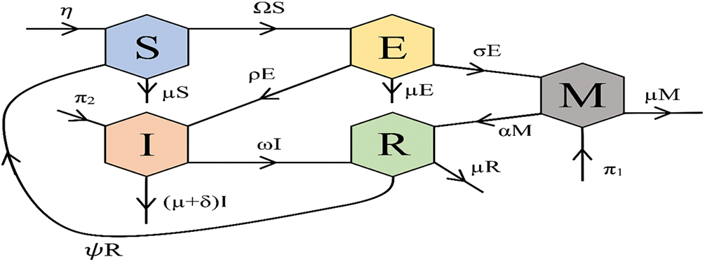
Figure 1: Flowchart of the model

The fuzzy model corresponding to the above model is given by

{dSdt=η−ΩS+ψR−μS,dEdt=ΩS−(μ+ρ+σ)E,dMdt=σE+π1−(μ+α)M,dIdt=ρE+π2−(μ+δ(x)+ω(x))I,dRdt=ω(x)I+αM−(μ+ψ)R.(4)

The susceptible animals (S) are recruited at a constant rate η and are subject to natural mortality at rate μ. Exposed animals (E) progress to symptomatic (I) or asymptomatic (M) infectious states at rates σ and ρ, respectively. The recovery rates for asymptomatic animals are α. α precisely can accurately simulate and predict the impact of asymptomatic individuals on disease transmission and recovery dynamics This parameter measures the proportion of infected people who do not show any symptoms of the disease and are recovering from the infection. The influx rates of asymptomatic and symptomatic animals from other regions are π1 and π2, respectively. The rate of disease transmission modified by ϕ, death due to the disease among infected animals, and recovery rate from the disease, are treated as fuzzy numbers owing to their uncertain nature. These parameters are represented by β(x), δ(x), and ω(x), respectively. The force of infection Ω is calculated based on transmission rate as Ω=β(x)(M+φI). Fuzzy variables like β(x), δ(x), and ω(x) embody uncertainty in mathematical simulations through the use of fuzzy models from the deterministic models. These variables are defined by the fuzzy numbers and their effect is described using the fuzzy differential equations and numerical solutions for the fuzzy systems. The result is a model that generates outcomes that can include several different values, as a result of the variability of the parameters involved. The fuzzy parameters mentioned in [48] and their definitions are provided below:

β(x)={0,x≤xmin,x−xminxmax−xmin,xmin<x≤xmax,1,xmax≤x,(5)

where xmin is the minimum value of the variable x where the function β(x), δ(x), and ω(x) transition. xmax is the maximum value of the variable x where the function β(x) transitions to a constant value.

δ(x)={(1−ξ)−a0xminx+a0,0≤x≤xmin,1−ξ,xmin<x,(6)

where a0 is a constant parameter in the function δ(x) that helps define the linear relationship for x in the interval 0≤x≤xmin and ξ is a constant parameter in δ(x) representing a fixed value that the function attains when xmin<x.

and

ω(x)=(ω0−1)xmaxx+1.0≤x≤xmin.(7)

where ω0 is a constant parameter in δ(x) that determines the slope of the linear function in the interval 0≤x≤xmin.

2.6 Fuzzy Delayed Model

Delayed epidemic models are critical for understanding and forecasting the dynamics of infectious illnesses when there is a considerable latency interval between infection and the commencement of infectiousness. The symbol τ denotes the latency period, which represents the time it takes for infected individuals to become contagious. The inclusion of e−μτ assumes a linear decrease in population over that specific duration, reflecting factors such as mortality or recovery, governed by μτ. The respective fuzzy epidemic model becomes the fuzzy delayed epidemic model by incorporating the (t−τ)e−μτ factor within susceptible and exposed animals’ compartments. The proposed fuzzy delayed epidemic model of FMD is given below:

{dSdt=η−ΩS(t−τ)e−μτ+ψR−μS,dEdt=ΩS(t−τ)e−μτ−(μ+ρ+σ)E,dMdt=σE+π1−(μ+α)M,dIdt=ρE+π2−(μ+δ(x)+ω(x))I,dRdt=ωI+αM−(μ+ψ)R.(8)

2.7 Equilibrium Analysis

Case 1: If x≤xmin we obtain

Ep0(S0,E0,M0,I0,R0)=(ημ,0,0,0,0).

Case 2: If xmin<x≤xmax, we have β(x)= x−xminxmax−xmin and Ep∗(S∗,E∗,M∗,I∗,R∗) we obtain

S∗=η+ψRβ(x)Ω∗e−μτ+μ,

E∗=β(x)Ω∗e−μτS∗k1,

M∗=σE∗+π1k2,

I∗=ρE∗+π2k3,

R∗=ω(x)I∗+αM∗k4.

Case 3: If xmax≤x we have β(x)=1 and Ep∗∗(S∗∗,E∗∗,M∗∗,I∗∗,R∗∗) we obtain

S∗∗=η+ψRΩ∗∗e−μτ+μ,

E∗∗=Ω∗∗e−μτS∗∗k1,

M∗∗=σE∗∗+π1k2,

I∗∗=ρE∗∗+π2k3,

R∗∗=ω(x)I∗∗+αM∗∗k4.

k4=(μ+ψ).

2.8 The Fuzzy Basic Reproductive Number (FBRN) ℛ0f

The FBRN number ℛ0 is calculated by utilizing a next-generation approach

ℛ0=β(x)ηe−μτ(δ(x)σ+αφρ+μφρ+ω(x)σ+μσ)μk1k2k3.(9)

The FBRN number ℛ0 can be analyzed as below:

Case 1: If x<xmin, then β(x)=0 we obtain

ℛ0(x)=0.

Case 2: If xmin<x≤xmax,we have β(x)= x−xminxmax−xmin we obtain

ℛ0(x)=β(x)ηe−μτ(δ(x)σ+αφρ+μφρ+ω(x)σ+μσ)μk1k2k3.

Case 3: xmax≤x we have β(x)=1 we obtain

ℛ0(x)=ηe−μτ(δ(x)σ+αφρ+μφρ+ω(x)σ+μσ)μk1k2k3.

ℛ0(x) can be written as

ℛ0(x)=(0,β(x)ηe−μτ(δ(x)σ+αφρ+μφρ+ω(x)σ+μσ)μk1k2k3,ηe−μτ(δ(x)σ+αφρ+μφρ+ω(x)σ+μσ)μk1k2k3).

The fuzzy reproductive number can be written as [49]

ℛ0f=E[ℛ0(x)],

where E[ℛ0(x)]=a+2b+c4,

and a=ℛ0(x) at Case 1, b=ℛ0(x) at Case 2, and c=ℛ0(x) at Case 3

ℛ0f=E[ℛ0(x)]=(0+2(β(x)ηe−μτ(δ(x)σ+αφρ+μφρ+ω(x)σ+μσ)μk1k2k3)+(ηe−μτ(δ(x)σ+αφρ+μφρ+ω(x)σ+μσ)μk1k2k3))4,

ℛ0f=ηe−μτ(δ(x)σ+αφρ+μφρ+ω(x)σ+μσ)(2β(x)+1)4μk1k2k3.(10)

2.9 Stability Analysis

The Jacobian matrix of system (6) at disease free equilibrium (DFE) is given by

J(Ep0)=[−μ00000−k10000σ−k2000ρ0−k3000αω(x)−k4].

The eigen values of the matrix are; λ1=−k2, λ2=−k4 ,λ3=−k3, λ4=−k1, λ5=−μ. As all the eigenvalues are less than zero, therefore, we concluded that the system of differential equations of the SEMIR model is locally asymptotically stable at Ep0.

3  Numerical Modelling

Numerical modeling is the application of mathematical equations and computing tools to simulate and analyze complicated systems or processes, resulting in predictions and insights that are frequently impossible to achieve from direct investigation. To solve the discretized governing equations of a system, computational techniques and algorithms like finite difference and finite element approaches are used. In this section, we can employ the forward Euler scheme and nonstandard finite difference methods for a given model.

3.1 Forward Euler Scheme

The Forward Euler method is an easily recognizable numerical method belonging to the first-order category and limited to the explicit class of method that operates in ordinary differential equations. Indeed, we present a forward Euler scheme for the described above system (8) as follows:

Sn+1=Sn+h(η−ΩSne−μτ+ψRn−μSn),(11)

En+1=En+h(ΩSne−μτ−(μ+ρ+σ)En),(12)

Mn+1=Mn+h(σEn+π1−(μ+α)Mn),(13)

In+1=In+h(ρEn+π2−(μ+δ(x)+ω(x))In),(14)

Rn+1=Rn+h(ω(x)In+αMn−(μ+ψ)Rn).(15)

3.2 NSFD Scheme

The NSFD method is used in epidemic models to solve differential equations numerically with high efficiency while preserving essential features of the continuous model. According to [50], NSFD schemes maintain the positivity and stability of solutions and converge numerically, making them suitable for epidemic studies. In general, NSFD schemes are cheaper in terms of computational cost than other approaches such as the forward Euler approach, and possess structural stability about the continuous model. The proposed fuzzy delayed nonstandard finite difference (FDNSFD) is given by

{Sn+1=Sn+h(η+ψRn)1+h(Ωe−μτ+μ),En+1=En+h(ΩSne−μτ)1+hk1,Mn+1=Mn+h(σEn+π1)1+hk2,In+1=In+h(ρEn+π2)1+hk3,Rn+1=Rn+h(ω(x)In+αMn)1+hk4.(16)

3.3 Positivity of FDNSFD

Considering the numerical methods to solve epidemic model equations, it’s important to preserve this positivity to get accurate and relevant results. In compartmental epidemic models, all state variables that represent population segments must have at least one positive value concerning other state variables that are non-negative throughout the analysis. It is important to keep these variables positive. This fundamental property is proved using the mathematical induction principle for an implicit numerical integration. The following theorem is useful:

Theorem: Let S, E, M, I and R are positive at t=0; furthermore, if ∝≥0, δ(x)≥0,μ≥0,ω(x)≥0,σ≥0,φ≥0,τ≥0 and β(x)≥0 then S(n+1)≥0, E(n+1)≥0, M(n+1)≥0, I(n+1)≥0 and R(n+1)≥0, for all n∈Z+.

{Sn+1=Sn+h(η+ψRn)1+h(Ωe−μτ+μ),En+1=En+h(ΩSne−μτ)1+hk1,Mn+1=Mn+h(σEn+π1)1+hk2,In+1=In+h(ρEn+π2)1+hk3,Rn+1=Rn+h(ω(x)In+αMn)1+hk4.(17)

Proof: For n=0 system (17) becomes

{S1=S0+h(η+ψR0)1+h(Ωe−μτ+μ)≥0,E1=E0+h(ΩS0e−μτ)1+hk1≥0,M1=M0+h(σE0+π1)1+hk2≥0,I1=I0+h(ρE0+π2)1+hk3≥0,R1=R0+h(ω(x)I0+αM0)1+hk4≥0.(18)

Now for n=1 system (17) becomes

{S2=S1+h(η+ψR1)1+h(Ωe−μτ+μ)≥0,E2=E1+h(ΩS1e−μτ)1+hk3≥0,M2=M1+h(σE1+π1)1+hk1≥0,I2=I1+h(ρE1+π2)1+hk2≥0,R2=R1+h(ω(x)I1+αM1)1+hk4≥0.(19)

Assume that the preceding set of equations guarantees that the values of S,E,M,I, andR have the property of positivity for n=2,3,4,…,n−1. In other words, for n=2,3,4,…,n−1, Sn+1≥0,En+1≥0,Mn+1≥0,In+1≥0and Rn+1≥0. The positivity will now be investigated for a random positive integer n, and we find that

{Sn+1=Sn+h(η+ψRn)1+h(Ωe−μτ+μ)≥0,En+1=En+h(ΩSne−μτ)1+hk1≥0,Mn+1=Mn+h(σEn+π1)1+hk2≥0,In+1=In+h(ρEn+π2)1+hk3≥0,Rn+1=Rn+h(ω(x)In+αMn)1+hk4≥0.(20)

Obviously, Sn+1≥0,En+1≥0,Mn+1≥0,In+1≥0, and Rn+1≥0, hence the proof.

3.4 Boundedness of the FDNSFD Scheme

Given that the model is about the human population, it is critical to ensure that at any given time ‘t’, the sum of populations in all compartments does not exceed the overall population. The following theorem addresses this condition effectively:

Theorem: Let S,E,M,I, and R≥0 be finite S+E+M+I+R≤N; furthermore, ∝ ≥0, δ(x)≥0,μ≥0,ω(x)≥0,σ≥0,φ≥0,τ≥0, and β(x)≥0 and then there is a constant such that Sn+1+En+1+In+1+Mn+1+Rn+1≤Nn for all n∈Z+.

Proof: For bondedness of the proposed FDNSFD scheme from the above system (16) we have

Sn+1(1+h(Ωe−μτ+μ))+En+1(1+h(µ+ρ+σ))+Mn+1(1+h(μ+α))+In+1(1+h(µ+δ(x)+ω(x)))+Rn+1(1+h(µ+ψ))=Sn+h(η+ψRn)+En+h(ΩSne−μτ)+Mn+h(σEn+π1)+In+h(ρEn+π2)+Rn+h(ω(x)In+αMn).(21)

(Sn+1+In+1+En+1+Rn+1)(1+hμ)+hΩe−μτ+h(ρ+σ+α+δ(x)+ω(x)+ψ)=(Sn+In+En+Rn)+h(η+ψRn+ΩSne−μτ+σEn+π1+ρEn+π2+ω(x)In+αMn).(22)

(Sn+1+En+1+Mn+1+In+1+Rn+1)+C=(Sn+En+Mn+In+Rn)+h(η+ψRn+ΩSne−μτ+σEn+π1+ρEn+π2+ω(x)In+αMn)(1+hμ).(23)

Now for n=0 system (23) becomes

(S1+E1+M1+I1+R1)+C=(S0+E0+M0+I0+R0)+h(η+ψR0+ΩS0e−μτ+σE0+π1+ρE0+π2+ω(x)I0+αM0)(1+hμ).

Since N1=S0+E0+M0+I0+R0,S1+E1+M1+I1+R1≤N1.

Similarly, for nϵZ+, the system (23) becomes

(Sn+1+En+1+Mn+1+In+1+Rn+1)+C=(Sn+En+Mn+In+Rn)+h(η+ψRn+ΩSne−μτ+σEn+π1+ρEn+π2+ω(x)In+αMn)(1+hμ).

Consequently, Sn+1≤Nn,En+1≤Nn,Mn+1≤NnIn+1≤NnandRn+1≤Nn, hence the proof.

3.5 Convergence Analysis

Convergence analysis in epidemic models determines the stability and accuracy of numerical approaches for solving disease spread differential equations. It determines if the numerical solution approaches the genuine solution when the computational parameters drop, assuring simulation reliability and accuracy while preserving the continuous model’s characteristics.

To prove this, assume that

F1=S+h(η+ψR)1+h(Ωe−μτ+μ),

F2=E+h(ΩSe−μτ)1+hk1,

F3=M+h(σE+π1)1+hk2,

F4=I+h(ρE+π2)1+hk3,

F5=R+h(ω(x)I+αM)1+hk4.

The Jacobean matrix corresponding to the above system at Ep0 is

J(Ep0)=[11+hμ000hω(x)1+hμ0011+hk1000hσ1+hk2011+hk200hρ1+hk311+hk30000hω(x)1+hk4hα1+hk411+hk4].

Eigen values of above Jacobian matrix, λ1=0.83333333<1, λ2=0.58823529<1, λ3=0.79835766<1, λ4=0.7167745<1 and λ5=0.08158315<1. All of the Jacobian matrix’s eigenvalues will be inside a unit circle, ensuring that the proposed FDNSFD scheme converges at point Ep0.

3.6 Consistency of the FDNSFD Scheme

Consistency refers to the numerical method’s ability to properly estimate the underlying continuous model when computing factors, such as step size, decrease. The findings of the search emphasize how crucial it is to preserve consistency in FDNSFD schemes to guarantee the dependability and precision of numerical solutions.

Beginning with the first equation in the system (16), we get

Sn+1(1+h(Ωe−μτ+μ))=Sn+h(η+ψRn).(24)

The Taylor’s series expansion of the Sn+1 is as follows:

Sn+1=(Sn+hdSdt+h22!d2Sdt2+h33!d3Sdt3+…).(25)

Substituting the value of Sn+1 in (24) we obtain

(Sn+hdSdt+h22!d2Sdt2+h33!d3Sdt3+…)(1+h(Ωe−μτ+μ)=Sn+h(η+ψRn).

After some simplification and apply h→0, we get

Sn(Ωe−μτ+μ)+dSdt=η+ψRn,

dSdt=η+ψRn−ΩSne−μτ−μSn,

⟹dSdt=η+ψR−ΩSe−μτ−μS.

From the second equation of the FDNSFD scheme, we have

En+1(1+hk1)=En+h(ΩSne−μτ).(26)

The Taylor’s series expansion of the En+1 is as follows:

En+1=(En+hdEdt+h22!d2Edt2+h33!d3Edt3+…).(27)

Substituting the value of En+1 in (26), we obtain

(En+hdEdt+h22!d2Edt2+h33!d3Edt3+…)(1+hk1)=En+h(ΩSne−μτ).

Apply h→0, we get

k1En+dEdt=ΩSne−μτ,

dEdt=ΩSne−μτ−k1En,

⟹dEdt=ΩSe−μτ−k1E.

From the third equation of the FDNSFD scheme, we have

Mn+1(1+hk2)=Mn+h(σEn+π1),(28)

The Taylor’s series expansion of the Mn+1 is as follows:

Mn+1=(Mn+hdMdt+h22!d2Mdt2+h33!d3Mdt3+…).(29)

Substituting the value of Mn+1 in (28), we obtain

(Mn+hdMdt+h22!d2Mdt2+h33!d3Mdt3+…)(1+hk2)=Mn+h(σEn+π1).

Apply h→0, we get

Mnk2+dMdt=σEn+π1,

dMdt=σEn+π1−k2Mn,

⟹dMdt=σE−M(σ+δ+μ).

From the fourth equation of the FDNSFD scheme, we have

In+1(1+hk3)=In+h(ρEn+π2).(30)

The Taylor’s series expansion of the In+1 is as follows:

In+1=(In+hdIdt+h22!d2Idt2+h33!d3Idt3+…).(31)

Substituting the value of In+1 in (30), we obtain

(In+hdIdt+h22!d2Idt2+h33!d3Idt3+…)(1+hk3)=In+h(ρEn+π2),

Apply h→0, we get

k3In+dIdt=ρEn+π2,

dIdt=ρEn+π2−k3In,

⟹dIdt=ρE+π2−k3I.

From the fourth equation of the FDNSFD scheme, we have

Rn+1(1+hk4)=Rn+h(ω(x)In+αMn).(32)

The Taylor’s series expansion of the Rn+1 is as follows:

Rn+1=(Rn+hdRdt+h22!d2Rdt2+h33!d3Rdt3+…).(33)

Substituting the value of Rn+1 in (32), we obtain

(Rn+hdRdt+h22!d2Rdt2+h33!d3Rdt3+…)(1+hk4)=Rn+h(ω(x)In+αMn).

Apply h→0, we get

k4Rn+dRdt=ω(x)In+αMn,

dRdt=ω(x)In+αMn−k4Rn,

⟹dRdt=ω(x)I+αM−k4R.

which shows that our proposed scheme is consistent with Order 1.

4  Mathematical Simulations

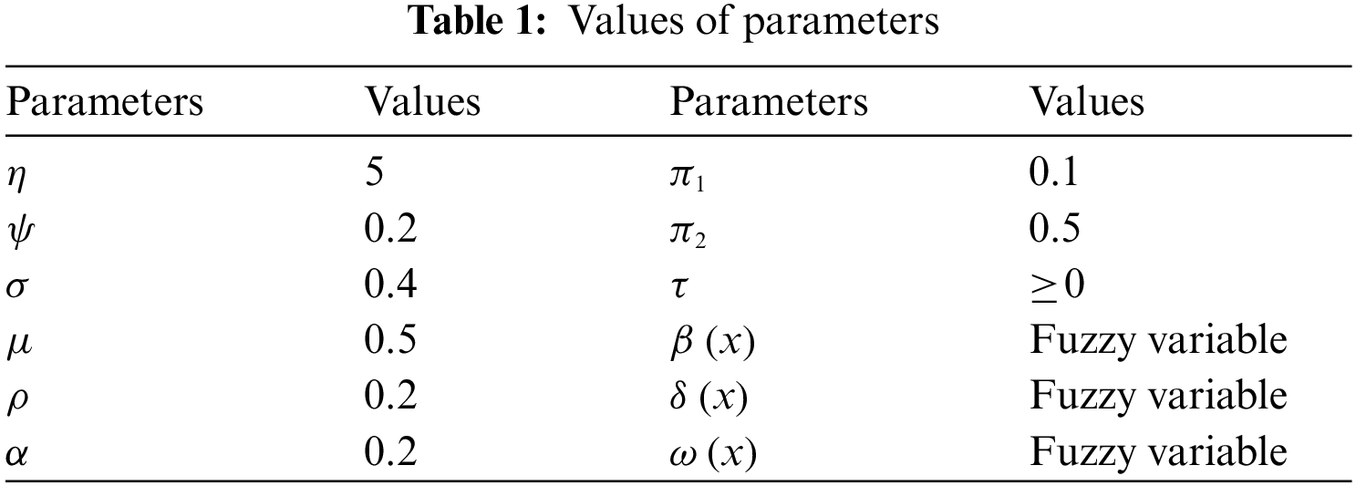
Table 1 outlines the parameters employed in numerical simulations.

In Fig. 2, the exposed population using the forward approach at different step sizes gives rise to non-physical oscillations, and negative values are not physically meaningful for compartments of the population.

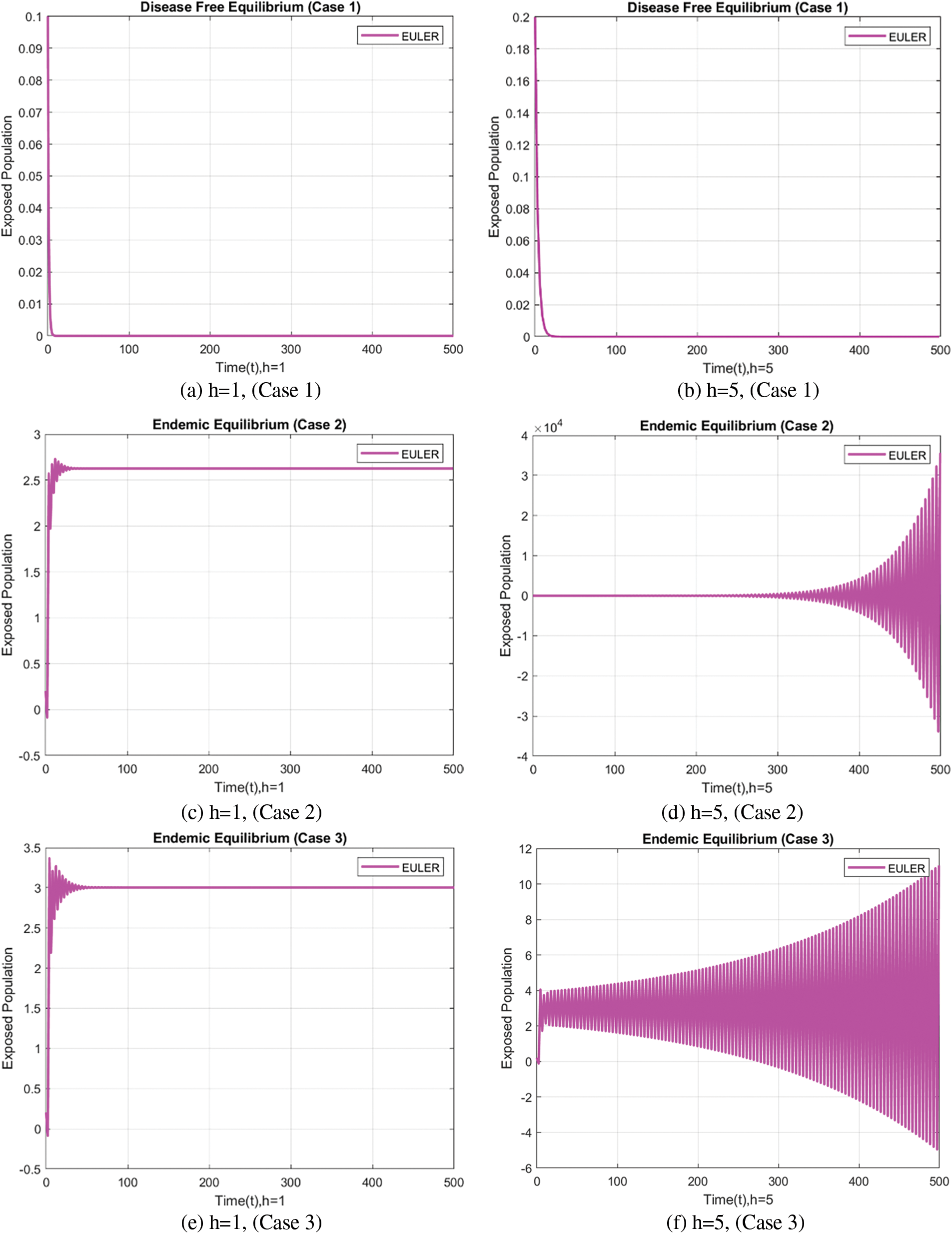
Figure 2: Exposed population at varying step sizes using the forward Euler approach

The behavior of the infected population is depicted in Fig. 3, which also includes signs of non-physical oscillations and negative values for the number of infected individuals, similar to the number of exposed individuals using the forward Euler approach.

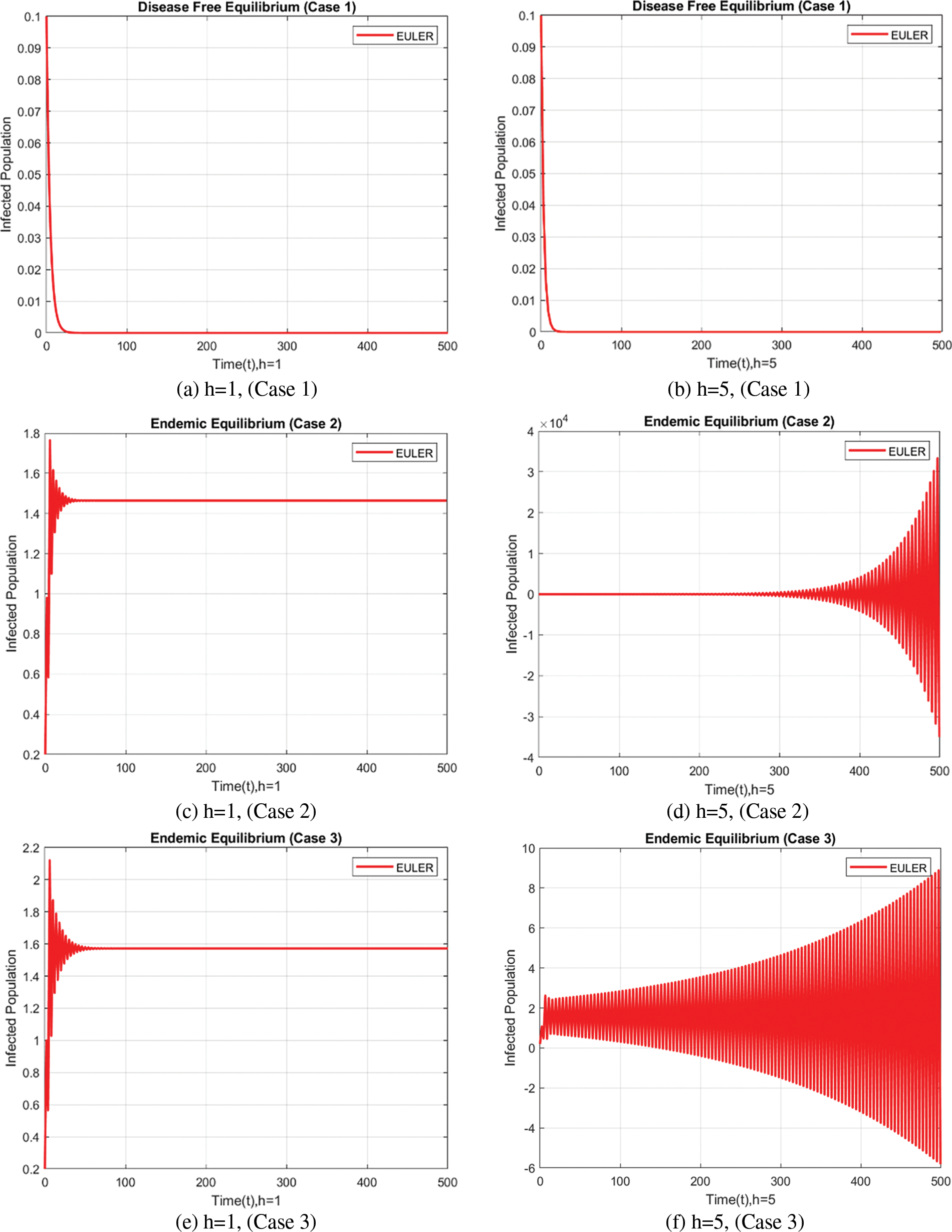
Figure 3: Infected populations at varying step sizes using the forward Euler approach

The graphical representation of the behavior of all compartments of the FMD virus model is presented in Fig. 4.

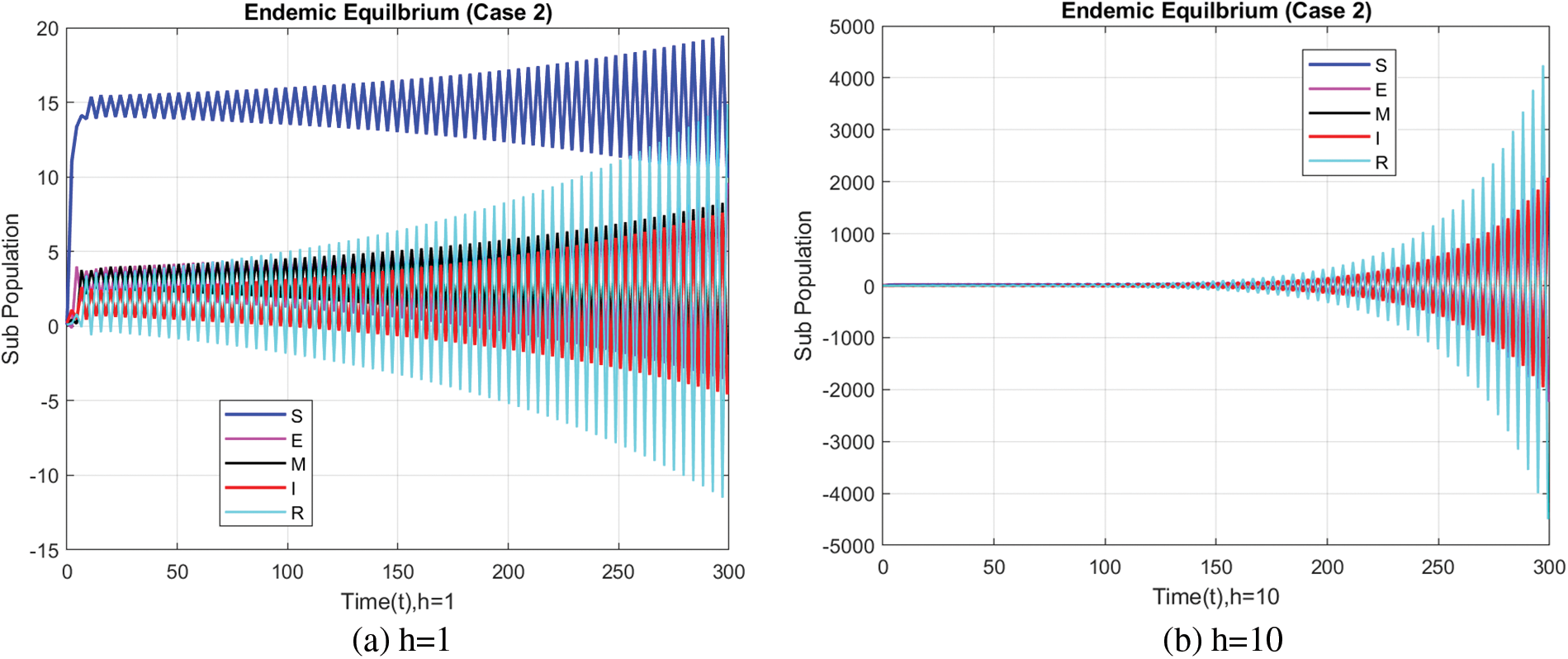
Figure 4: Compartmental analysis of the SEMIR model using the forward Euler approach

In this case, Fig. 5 illustrates the behavior of the exposed population using the FDNSFD scheme approach employing different step sizes. This method prevents negativities and yields the expected outcomes.

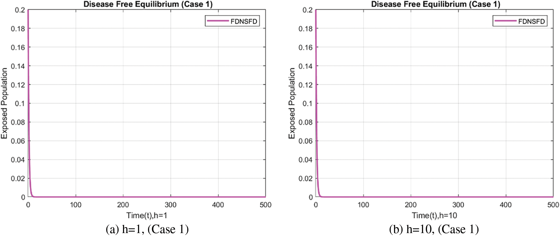
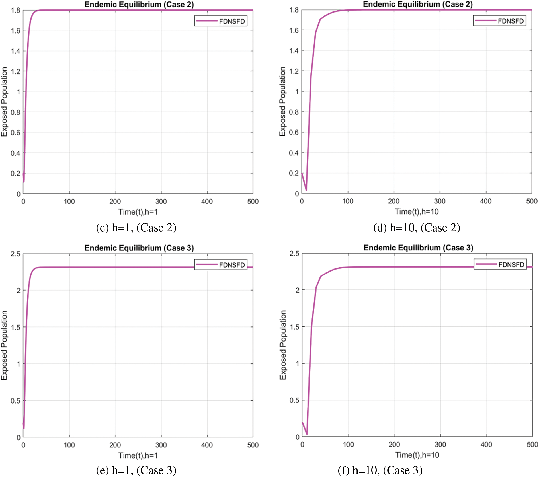
Figure 5: Exposed population at varying step sizes using the FDNSFD approach

Fig. 6 portrays the infected population at different step sizes with the FDNSFD method that gives mainly positive values and outcomes, as the infected population does.

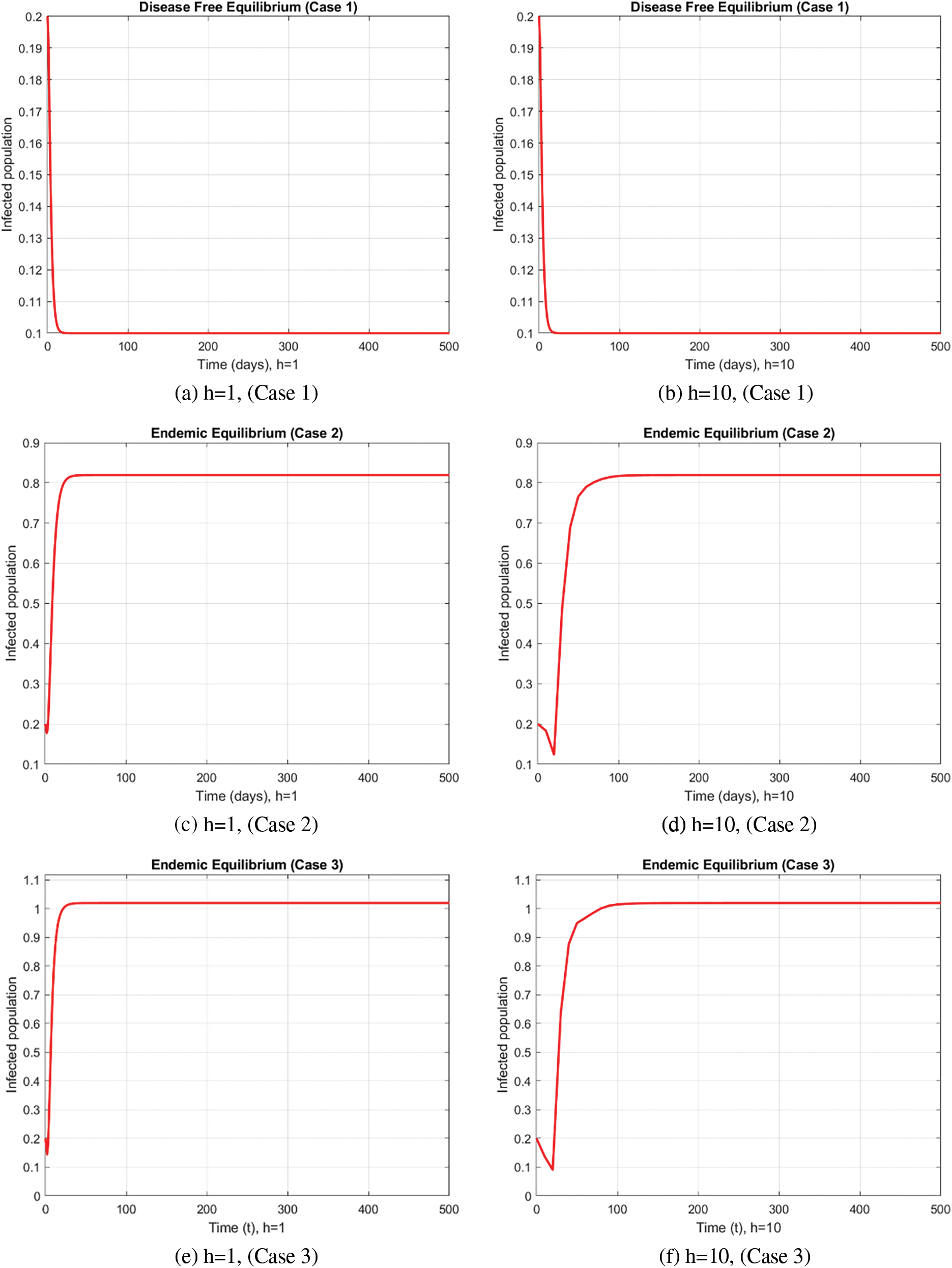
Figure 6: Infected population at varying step sizes using the FDNSFD approach

Fig. 7 shows the state of all compartments of the SEIMR model under consideration using the FDNSFD method.

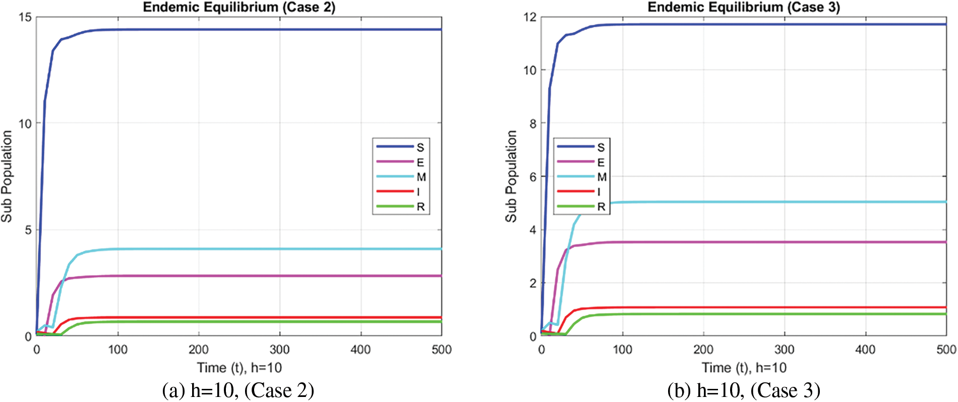
Figure 7: Compartmental analysis of the SEMIR model using the FDNSFD approach

In the case of the FDNSFD approach, the behavior of the exposed and infected population is explained for each case in Fig. 8. The exposed and infected population for each scenario based on the FDNSFD approach is represented. Which shows an escalating infection rate in all cases. As for Case 1, it is possible to observe almost the complete absence of disease, whereas Cases 2 and 3 describe an endemic equilibrium, although with a higher infection rate in Case 3 compared to Case 2.

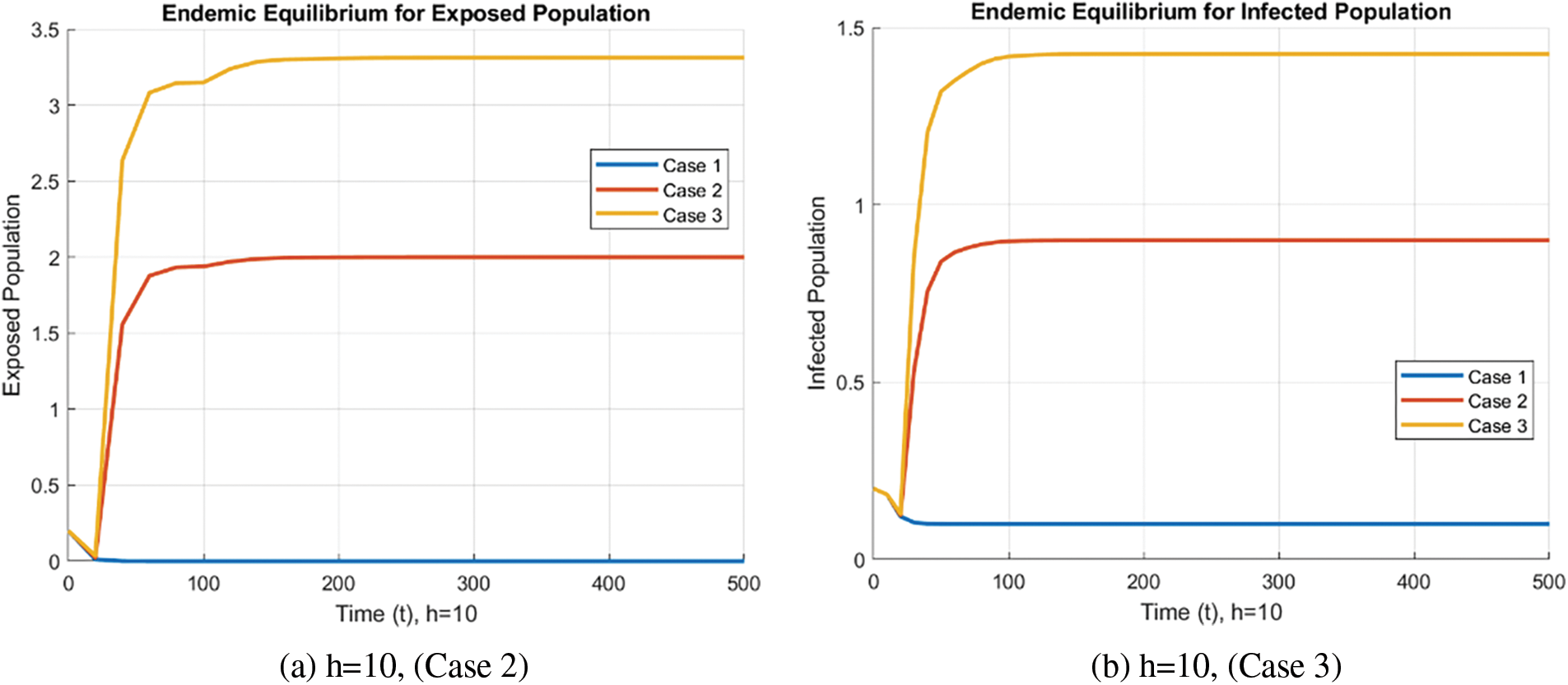
Figure 8: Exposed and Infected population in each case using the FDNSFD approach

The exposed and infected population for a detailed fuzzy delayed NSFD model with/without a delay factor is presented in the form of Fig. 9. The graph helps to show that, the introduction of a delay factor reduces the spread of the disease and thus, the number of people affected by FMD.

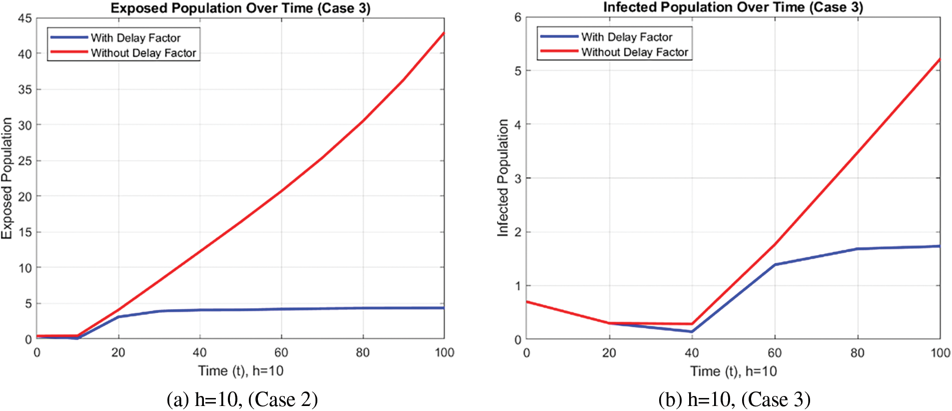
Figure 9: Effect of time delay on infected population using FDNSFD approach

Fig. 10 illustrates the effect of τ on the exposed and infected population while using the FDNSFD approach. This simulation illustrates that increasing the value of results significantly in slowing down the process of spread.

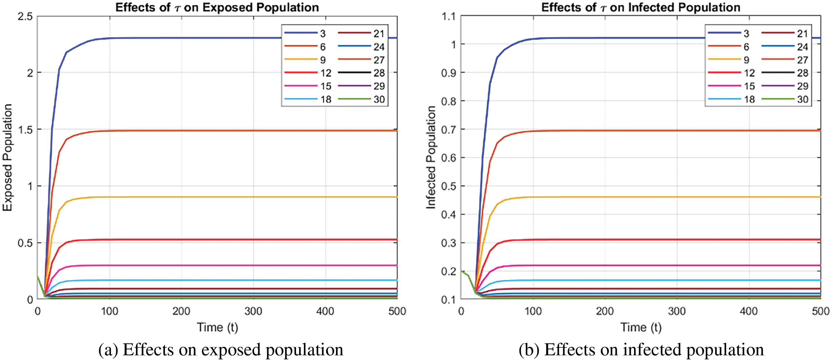
Figure 10: Effect of time delay τ on exposed and infected population

Overall, the NSFD approach excels in modeling population dynamics, delivering realistic and reliable results while avoiding the non-physical outcomes linked to the forward approach.

5  Conclusion

This paper investigates FMD transmission by including the contribution of efficient active migrants in its mathematical model. Based on the improved SEMIR model, which has incorporated the time delays into the analysis while adopting the forward Euler method and the FDNSFD approach to study disease spread. From the discoveries made in the chapter, there is more information that we can use. Still, at the same time, the forward Euler method has drawbacks: the non-physical oscillations and negative values, which are irrelevant to the population compartments. The FDNSFD method as compared to the Euler method cumulatively integrates fuzzy logic for uncertainty and time delay for delayed reactions in a system. The FDNSFD is well applicable in complicated and stochastic situations, while the Euler method, despite its simplicity and popularity, can fail erratically and inaccurately in such cases.

On the other hand, the approach used in the formalization of a problem coping with such challenges is positive and provides realistic solutions. This is supported by the graphical analyses provided in this work, where it was established that FDNSFD arrests the issue of negativity and gives an exponential-like behavior for exposed and infected populations under different scenarios and step sizes. One is to note that adding a delay factor within the FDNSFD improves the result by greatly decreasing the spreading of FMD, indicating the effect of the time delays in the epidemiological model. The current paper outlines that in enhancing the FDNSFD method, the most important properties that define the continuous model are all captured, producing a reliable model for disease dynamics. In conclusion, the FDNSFD approach turns out to be a better method of modeling the spread of FMD than the traditional techniques, which give more confident and precise results. This has a variety of implications for FMD management and possibly the development of better interventions to control the incidence. Further research should expand on the development and refinement of the fuzzy logic and numerical algorithms used in the models of other infectious diseases so that the application of such models for increasing disease knowledge and control may be enhanced.

Limitation of study: The model has some assumptions that may not capture the true nature of FMD transmission, such as the equal distribution of people. From experience, the more data that is available, the more credible a model will be; if there is inaccuracy in the data collected or acts of omission in the same, then the model will yield an inaccurate result. Nevertheless, the FDNSFD is beneficial for use, and the method is computationally more intensive than the conventional methods, which may become a limitation in today’s world of limited resources. The generalizability of the results and the potential of applying the given model to other areas or cultures is also somewhat limited by the fact that they have to be fine-tuned and recalibrated if tested on local data. The values of model parameters may be uncertain, and if this is the case, then the stability and the accuracy of the model may be compromised. Future works should extend the development and analysis of the fuzzy logic and the numerical formulas used in the models of other forms of infectious disease so that the benefit of such models for the development of disease information as well as the prevention of diseases could be improved.

Acknowledgement: The authors Thabet Abdeljawad and Aiman Mukheimer would like to thank Prince Sultan University for paying the APC and for the support through TAS research lab.

Funding Statement: This research received no specific grant from any funding agency in the public, commercial, or not-for-profit sectors.

Author Contributions: Conceptualization, methodology, software, and draft manuscript preparation: Muhammad Tashfeen and Fazal Dayan; Formal analysis, methodology, software, validation, and supervision: Muhammad Aziz ur Rehman, Thabet Abdeljawad and Aiman Mukheimer. All authors reviewed the results and approved the final version of the manuscript.

Availability of Data and Materials: The data presented in this article are available from the corresponding author upon reasonable request.

Ethics Approval: Not applicable.

Conflicts of Interest: The authors declare that they have no conflicts of interest to report regarding the present study.

References

1. Bernoulli D, Chapelle D. Essai d’une nouvelle analyse de la mortalité causée par la petite vérole, et des avantages de l’inoculation pour la prévenir; 2023. Available from: https://inria.hal.science/hal-04100467/. [Accessed 2024]. [Google Scholar]

2. Ross R. The prevention of malaria. London: John Murray; 1911. [Google Scholar]

3. Kermack WO, McKendrick AG. Contributions to the mathematical theory of epidemics–I. 1927. Bull Math Biol. 1991;53(1–2):33–55. doi:10.1007/BF02464423 [Google Scholar] [PubMed] [CrossRef]

4. van den Driessche P, Watmough J. Reproduction numbers and sub-threshold endemic equilibria for compartmental models of disease transmission. Math Biosci. 2002;180(1–2):29–48. doi:10.1016/S0025-5564(02)00108-6 [Google Scholar] [PubMed] [CrossRef]

5. En’Ko PD. On the course of epidemics of some infectious diseases; 1989. Available from: https://www.cabidigitallibrary.org/doi/full/10.5555/19902069796. [Accessed 2024]. [Google Scholar]

6. Brauer F, Castillo-Chavez C, Feng Z. Mathematical models in epidemiology. New York: Springer; 2019. vol. 32. [Google Scholar]

7. Buonomo B, Chitnis N, d’Onofrio A. Seasonality in epidemic models: a literature review. Ricerche di Matematica. 2018;67(1):7–25. doi:10.1007/s11587-017-0348-6. [Google Scholar] [CrossRef]

8. Buonomo B, Lacitignola D, Vargas-De-León C. Qualitative analysis and optimal control of an epidemic model with vaccination and treatment. Math Comput Simul. 2014;100(6):88–102. doi:10.1016/j.matcom.2013.11.005. [Google Scholar] [CrossRef]

9. Hethcote HW. The mathematics of infectious diseases. SIAM Rev. 2000;42(4):599–653. doi:10.1137/S0036144500371907. [Google Scholar] [CrossRef]

10. Martin DL, Gustafson TL, Pelosi JW, Suarez L, Pierce GV. Contaminated produce—a common source for two outbreaks of Shigella gastroenteritis. Am J Epidemiol. 1986;124(2):299–305. doi:10.1093/oxfordjournals.aje.a114388 [Google Scholar] [PubMed] [CrossRef]

11. Swaddiwudhipong W, Karintraratana S, Kavinum S. A common-source outbreak of shigellosis involving a piped public water supply in northern Thai communities. J Trop Med Hyg. 1995;98:145–5 [Google Scholar] [PubMed]

12. Misra AK, Sharma A, Shukla JB. Modeling and analysis of effects of awareness programs by media on the spread of infectious diseases. Math Comput Model. 2011;53(5–6):1221–8. doi:10.1016/j.mcm.2010.12.005. [Google Scholar] [CrossRef]

13. Rihan FA. Delay differential equations and applications to biology. Singapore: Springer; 2021. p. 123–41. [Google Scholar]

14. Cooke KL, Yorke JA. Some equations modelling growth processes and gonorrhea epidemics. Math Biosci. 1973;16(1–2):75–101. doi:10.1016/0025-5564(73)90046-1. [Google Scholar] [CrossRef]

15. Smith HL. An introduction to delay differential equations with applications to the life sciences, New York: Springer; 2011. vol. 57, p. 119–30. [Google Scholar]

16. Brauer F, Castillo-Chavez C. Mathematical models for communicable diseases. Philadelphia, USA: Society for Industrial and Applied Mathematics; 2012. [Google Scholar]

17. Ghosh S, Volpert V, Banerjee M. An epidemic model with time delay determined by the disease duration. Mathematics. 2022;10(15):2561. doi:10.3390/math10152561. [Google Scholar] [CrossRef]

18. Meziane M, Moussaoui A, Volpert V. On a two-strain epidemic model involving delay equations. Math Biosci Eng. 2023;20(12):20683–711. doi:10.3934/mbe.2023915 [Google Scholar] [PubMed] [CrossRef]

19. Almuqati BM, Allehiany FM. Global stability of a multi-group delayed epidemic model with logistic growth. AIMS Math. 2023;8(10):23046–61. doi:10.3934/math.20231173. [Google Scholar] [CrossRef]

20. Ma Z. Dynamical modeling and analysis of epidemics. Singapore: World Scientific; 2009. [Google Scholar]

21. Beretta E, Hara T, Ma W, Takeuchi Y. Global asymptotic stability of an SIR epidemic model with distributed time delay. Nonlinear Anal. 2001;47(6):4107–15. doi:10.1016/S0362-546X(01)00528-4. [Google Scholar] [CrossRef]

22. Tipsri S, Chinviriyasit W. The effect of time delay on the dynamics of an SEIR model with nonlinear incidence. Chaos Solitons Fractals. 2015;75:153–72. doi:10.1016/j.chaos.2015.02.017. [Google Scholar] [CrossRef]

23. Hussien RM, Naji RK. The dynamics of a delayed eco epidemiological model with nonlinear incidence rate. J Appl Math. 2023:2023(1):1366763. [Google Scholar]

24. Shatanawi W, Raza A, Arif MS, Rafiq M, Abodayeh K, Bibi M. An effective numerical method for the solution of a stochastic coronavirus (2019-nCoV) pandemic model. Comput Mater Contin. 2021;66(2):1121–37. doi:10.32604/cmc.2020.012070. [Google Scholar] [CrossRef]

25. Shoaib Arif M, Raza A, Abodayeh K, Rafiq M, Bibi M, Nazeer A. A numerical efficient technique for the solution of susceptible infected recovered epidemic model. Comput Model Eng Sci. 2020;124(2):477–91. doi:10.32604/cmes.2020.011121. [Google Scholar] [CrossRef]

26. Abodayeh K, Raza A, Arif MS, Rafiq M, Bibi M, Mohsin M. Stochastic numerical analysis for impact of heavy alcohol consumption on transmission dynamics of gonorrhoea epidemic. Comput Mater Contin. 2020;62(3):1125–42. doi:10.32604/cmc.2020.08885. [Google Scholar] [CrossRef]

27. Zimmermann H-J. Fuzzy set theory—and applications. 4th ed. Boston: Kluwer Academic Publishers; 2001. [Google Scholar]

28. Bates JH, Young MP. Applying fuzzy logic to medical decision making in the intensive care unit. Am J Respir Crit Care Med. 2003;167(7):948–52. doi:10.1164/rccm.200207-777CP [Google Scholar] [PubMed] [CrossRef]

29. Smithson M, Verkuilen J. Fuzzy set theory: applications in the social sciences. Thousand Oaks, CA: SAGE Publications; 2006. [Google Scholar]

30. Abdy M, Side S, Annas S, Nur W, Sanusi W. An SIR epidemic model for COVID-19 spread with fuzzy parameter: the case of Indonesia. Adv Differ Equ. 2021;2021(1):1–17. doi:10.1186/s13662-021-03263-6 [Google Scholar] [PubMed] [CrossRef]

31. Li C, Huang J, Chen YH, Zhao H. A fuzzy susceptible-exposed-infected-recovered model based on the confidence index. Int J Fuzzy Syst. 2021;23(4):907–17. doi:10.1007/s40815-020-01029-y. [Google Scholar] [CrossRef]

32. Shi X, Li J, Huang A, Song S, Yang Z. Assessing the outbreak risk of epidemics using fuzzy evidential reasoning. Risk Anal. 2021;41(11):2046–64. doi:10.1111/risa.13730 [Google Scholar] [PubMed] [CrossRef]

33. Chandrika P, Rajivganthi C. Control analysis of fractional-order extracellular delayed Hepatitis C virus model. Eur Phys J Spec Top. 2024 Jun 17. doi:10.1140/epjs/s11734-024-01202-6. [Google Scholar] [CrossRef]

34. Baleanu D, Dayan F, Ahmed N, Rafiq M, Raza A, Ahmad MO. Computational investigation of hand foot mouth disease dynamics with fuzziness. Comput Mater Contin. 2023 Jan 1;75(2):4175–89. doi:10.32604/cmc.2023.034868. [Google Scholar] [CrossRef]

35. Alqarni MM, Rafiq M, Dayan F, Awrejcewicz J, Ahmed N, Raza A, et al. New trends in fuzzy modeling through numerical techniques. Comput Mater Contin. 2023;74(3):6371–88. doi:10.32604/cmc.2023.033553. [Google Scholar] [CrossRef]

36. Dayan F, Ahmed N, Rafiq M, Iqbal MS, Khan I, Raza A, et al. A dynamically consistent approximation for an epidemic model with fuzzy parameters. Expert Syst Appl. 2022;210(6):118066. doi:10.1016/j.eswa.2022.118066. [Google Scholar] [CrossRef]

37. James AD, Rushton J. The economics of foot and mouth disease. OIE Rev Sci Tech. 2002;21(3):637–44. doi:10.20506/rst.21.3.1356 [Google Scholar] [PubMed] [CrossRef]

38. OEC. The Observatory of Economic Complexity (OEC); 2022. Available from: https://oec.world/en/profile/country/ury/. [Accessed 2022]. [Google Scholar]

39. Gibbens JC, Sharpe CE, Wilesmith JW, Mansley LM, Michalopoulou E, Ryan JB, et al. Descriptive epidemiology of the 2001 foot-and-mouth disease epidemic in Great Britain: the first five months. Vet Rec. 2001;149(24):729–43. doi:10.1136/vr.149.24.729. [Google Scholar] [CrossRef]

40. Bouma A, Elbers ARW, Dekker A, de Koeijer A, Bartels C, Vellema P, et al. The foot-and-mouth disease epidemic in the Netherlands in 2001. Prev Vet Med. 2003;57(3):155–66. doi:10.1016/S0167-5877(02)00217-9 [Google Scholar] [PubMed] [CrossRef]

41. Perez AM, Ward MP, Carpenter TE. Epidemiological investigations of the 2001 foot-and-mouth disease outbreak in Argentina. Vet Rec. 2004;154(25):777–82. doi:10.1136/vr.154.25.777 [Google Scholar] [PubMed] [CrossRef]

42. Ferguson NM, Donnelly CA, Anderson RM. Erratum: transmission intensity and impact of control policies on the foot and mouth epidemic in Great Britain. Nature. 2001;414:329. [Google Scholar]

43. Muroga N, Kobayashi S, Nishida T, Hayama Y, Kawano T, Yamamoto T, et al. Risk factors for the transmission of foot-and-mouth disease during the 2010 outbreak in Japan: a case-control study. BMC Vet Res. 2013;9(1):1–9. doi:10.1186/1746-6148-9-150 [Google Scholar] [PubMed] [CrossRef]

44. Yang PC, Chu RM, Chung WB, Sung HT. Epidemiological characteristics and financial costs of the 1997 foot-and-mouth disease epidemic in Taiwan. Vet Rec. 1999;145(25):731–4. doi:10.1136/vr.145.25.731 [Google Scholar] [PubMed] [CrossRef]

45. Ward MP, Perez AM. Herd demographics correlated with the spatial distribution of a foot-and-mouth disease epidemic in Buenos Aires province, Argentina. Prev Vet Med. 2004;65(3-4):227–37. doi:10.1016/j.prevetmed.2004.08.003 [Google Scholar] [PubMed] [CrossRef]

46. Boender GJ, van Roermund HJW, de Jong MCM, Hagenaars TJ. Transmission risks and control of foot-and-mouth disease in the Netherlands: spatial patterns. Epidemics. 2010;2(1):36–47. doi:10.1016/j.epidem.2010.03.001 [Google Scholar] [PubMed] [CrossRef]

47. Mfinanga IS, Shaban N, Marijani T. Modelling foot and mouth disease in the context of active immigrants. J Appl Math Phys. 2024;12(1):147–67. doi:10.4236/jamp.2024.121012. [Google Scholar] [CrossRef]

48. De Barros LC, Bassanezi RC, Lodwick WA. Fuzzy dynamical systems. In: A first course in fuzzy logic, fuzzy dynamical systems, and biomathematics. Studies in fuzziness and soft computing. Berlin, Heidelberg: Springer, 2016, vol. 347, p. 175–203. doi:10.1007/978-3-662-53324-6_8. [Google Scholar] [CrossRef]

49. Mangongo YT, Bukweli JDK, Kampempe JDB. Fuzzy global stability analysis of the dynamics of malaria with fuzzy transmission and recovery rates. Am J Oper Res. 2021;11(6):257–82. doi:10.4236/ajor.2021.116017. [Google Scholar] [CrossRef]

50. Alsaadi A, Dayan F, Ahmed N, Baleanu D, Rafiq M, Raza A. Evolutionary computational method for tuberculosis model with fuzziness. AIP Adv. 2023;13(8). doi:10.1063/5.0165348. [Google Scholar] [CrossRef]