Optimizing Bearing Fault Detection: CNN-LSTM with Attentive TabNet for Electric Motor Systems

1  Introduction

Manufacturing industrial machinery and equipment relies heavily on electric motor-driven systems [1]. Agribusiness, textiles, and transportation are among the industries that utilize these systems. As shown in Fig. 1 (https://uk.rs-online.com/web/generalDisplay.html?id=solutions/electric-motors-how, accessed on 30 July 2024), bearings are one of the most important parts of electric motors. The bearings are located near the exit point of the shaft and prevent direct contact between metal parts of the machine that are in relative motion. Doing so prevents friction, wear and tear, and overheating in electric motors. Despite their importance, machines and electronics driven by electric motors are susceptible to failures and faults [2]. Economic losses, productivity losses, environmental disasters, and even safety risks can be associated with any failure of these systems. The abovementioned concerns highlighted the need for timely and efficient fault diagnosis in electric motor-driven systems [3]. Early fault diagnosis can prevent economic losses and improve the reliability and performance of machines and equipment [4].

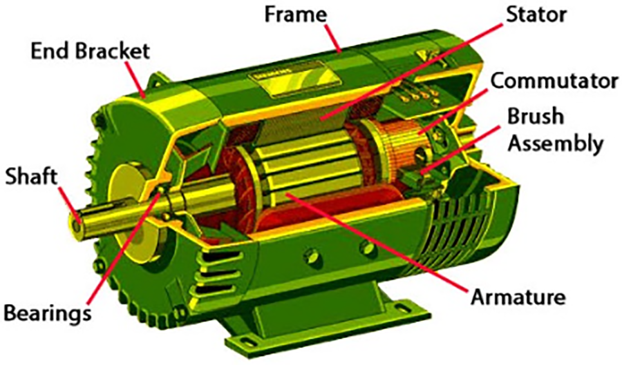
Figure 1: Parts of electric motors

Over the years, several traditional methods have been employed to tackle bearing fault diagnosis in electric motor-driven systems. The vibration analysis method [5] was used for the early fault detection and diagnosis in electrical motors. In this study, the authors analyzed the vibration spectrum created by the specific frequencies of electrical faults. The graphs were generated in MATLAB, and the model performed well. However, this paper gave no results for when the electric motor vibrates under all external forces. Another study [6] used the current signature analysis method to detect and diagnose faults in electric motors. This method works by analyzing the current waveforms generated by faulty motors. The results of this study showed efficient fault diagnosis. However, they could not perform under some abnormalities, such as incorrectly identifying gearbox components due to a broken rotor bar. Thermographic techniques were also introduced to diagnose faults in electrical and mechanical motors [7]. These techniques diagnosed faults with the help of infrared imaging by detecting overheated sections in the motor, which were the reason for potential faults.

Other methods utilized Acoustic Emission (AE) analysis to detect faults in electric motor-driven systems. This approach used AE signals to efficiently diagnose the faults by analyzing the variable rotational speed [8]. Expert systems were also among the traditional methods used for fault diagnosis in electric motors. In these systems, knowledge-based approaches were designed that utilized expert inputs and rules to detect machine faults [9]. While these traditional methods have been useful to some extent, they suffer from limitations such as reliance on domain expertise, inability to handle large datasets, and the need for manual feature extraction, which can be time-consuming and error-prone.

Electric motor-driven systems have been revolutionized in recent years by the advancement in machine and deep learning techniques. Various algorithms based on these techniques have been proposed and utilized for automated fault diagnosis. Support Vector Machine (SVM) algorithms have been used to detect and diagnose faults in electric motors. In a study [10], faults, including broken rotor bars, bearing faults, unbalanced rotors, and bowed and misaligned rotors, were efficiently diagnosed with the help of the SVM model. This study extracted and considered features like time domain features, eight moments, standard deviation, skewness, and kurtosis. Apart from the good performance, this study achieved diagnosis results against limited data cases. Decision trees with 22 classes were used to detect faults in open circuits of voltage source inverters. The model performed well on all the evaluation metrics and was considered an effective method for diagnosing inverter faults. However, the authors mentioned that the model’s performance should be assessed using multiple motor configurations [11].

Another efficient approach, Random Forest, was implemented to diagnose faults in line start-permanent magnet synchronous motor (LS-PMSM). The model detected faulty and healthy LS-PMSM well by combining the predictions of 1000 decision trees over all the extracted features. However, after comparing the results of random forests with other approaches, the authors concluded that other approaches also gave high accuracies; practitioners should be flexible in choosing the algorithm and not be limited to random forests [12]. The K-nearest algorithm (KNN) was then used to detect the fault and severity of that fault in three-phase induction motors. This algorithm worked by measuring the distance between query scenarios and accessing overall training metrics. The algorithm achieved high accuracy overall but was limited to three-phase induction motors only [13].

The Naive Bayes algorithm was also used to detect bearing faults in the induction motor. FFT (Fast Fourier Transform) analysis was also performed in this study. The bearing faults were categorized into distributed and localized faults. The model performed well and gave promising results compared to the SVM model. However, during the analysis, the rotator speed was not considered [14]. In another study, FFT analysis was combined with principal component analysis to diagnose faults in induction motors [15]. The FFT was used to analyze induction motors based on frequency domains. PCA (Principal Component Analysis) was used for feature selection. The study showed exceptional fault diagnosis results based on frequency and amplitude.

In another study, analysis of vibration signals was conducted using Convolutional Neural Networks (CNN) with Short-time Fourier Transforms (STFT) [16]. The STFT is a time-frequency-based feature map. The method was validated by simulating six different faults on an experimental bench. The results confirmed that this method could efficiently detect faults in electric motor-driven systems. An Autoencoder network was designed and implemented for fault diagnosis in electric motors. This study used deep neural networks and vibration signals to detect faults efficiently [17]. Compared with SVM, CNN, Multi-layer Perceptron (MLP), and other methods, this unsupervised model was considered the most effective for fault diagnosis. Some of the other useful approaches, such as LTSM [18] (Long Short-Term Memory Network) and RNN [19] (Recurrent Neural Network), were also used for fault diagnosis. While these machine and deep learning approaches have shown promising results, they still face challenges in dealing with highly complex and diverse motor-driven system data. Additionally, their performance heavily relies on appropriate feature engineering and hyperparameter tuning [20].

As a solution to these limitations, Deep Neural Networks (DNNs) emerged as a powerful subset of deep learning models that produce hierarchical representations based on raw data, eliminating the need to manually construct feature representations [21]. The use of these networks has shown remarkable success in various applications, including image and speech recognition and now fault diagnosis. An analysis of machinery fault diagnosis was presented in a study using a deep learning-based method based on domain generalization [22].

This paper proposes the development of a fine-tuned deep neural network tailored for efficient fault diagnosis in electric motors. By harnessing the power of deep neural networks to achieve heightened accuracy, robustness, and scalability in automated fault diagnosis of electric motor-driven systems, this advanced neural network significantly enhances fault diagnosis, reducing downtime, optimizing energy consumption, and bolstering industrial reliability. Such advancements hold transformative potential for diverse industries, including manufacturing, automation, and renewable energy, by improving overall productivity and maintenance strategies.

The research objective encompasses the following key aspects:

1.    Development of the Fine-Tuned TabNet Convolutional Neural Network Long Short-Term Memory (FTCNN-LSTM) Algorithm: To introduce the FTCNN-LSTM algorithm, a novel and comprehensive approach that merges Convolutional Neural Networks (CNNs) and Long Short-Term Memory (LSTM) networks with TabNet for efficient feature extraction, sequential modeling, and interpretability. This algorithm represents a significant methodological advancement in the field of fault diagnosis for electric motor-driven systems.

2.    Enhanced Pre-Processing Techniques: Another key objective is demonstrating the effectiveness of segmentation and normalization techniques, including Feature Scaling and label encoding, in pre-processing the Case Western Reserve University (CWRU) bearing fault data. These pre-processing methods are critical for improving the performance and reliability of the fault diagnosis model and contribute to the methodology.

3.    Optimized Model Architecture: To present an optimized model architecture that includes 1D Convolutional layer, batch normalization, max-pooling functions, LSTM blocks with dropout, batch normalization, dense layers, and appropriate activation and loss functions. The fine-tuning of this architecture prevents overfitting and is a noteworthy methodological contribution.

4.    Comparative Evaluation: To includes the comparative evaluation of the FTCNN-LSTM model against other established approaches, such as CNN, LSTM, CNN-LSTM combined with Random Forest, and CNN-LSTM with Gradient Boosting. This comparison, based on performance metrics, contributes methodological insights into the effectiveness of the proposed approach.

The remaining paper is prepared as the introduction summarizes the research problem and its significance, setting the stage for the study. The materials and methods section describes the study design, including the participants, data collection procedures, and statistical analysis. The results section explains the study’s outcomes, including tables and figures that help illustrate the data. The discussion section interprets the results, discussing their implications for the research question and identifying study limitations. Finally, the conclusion summarizes the main findings and their significance, highlighting any implications for future research.

2  Materials and Methods

2.1 Dataset Description

This study utilized the CWRU fault-bearing diagnosis dataset. Research studies using deep learning algorithms have used the CWRU fault-bearing diagnosis dataset to detect and diagnose machinery faults. The dataset includes 2 horse-power (HP) motors, dynamometers, torque sensors, and control electronics to evaluate motor performance. The faults presented in the dataset are intentionally introduced through electric spark-induced damage, which serves as controlled artificial damage.

•   “DE” indicates drive end data.

•   “FE” stands for fan end data.

•   “BA” indicates base accelerometer data.

•   “time” represents a time series of data.

•   “RPM” indicates the speed during measurement.

During the drive end-bearing experiments, vibration data from normal and faulty bearings were collected at 12,000 and 48,000 samples per second (samples/sec). Twelve thousand samples/sec were collected for all the Fan End (FE) bearing data. The dataset covers a range of defects and is classified into ten major classes, including healthy or normal motors, electric motors with ball faults, machines showing inner race faults, and motors with outer race faults. The outer race faults were recorded at 3, 6, and 12 o’clock positions, with defect diameters of 0.007, 0.014, and 0.021, respectively. The dataset corresponds to specific conditions: 1 HP motor load, 1772 RPM shaft speed, and a frequency of 48 kHz. There are nine selected parameters for fault identification prediction, including max, min, mean, standard deviation, kurtosis, crest factor, shaft speed/RMS, skewness, and form factor.

The CWRU fault-bearing diagnosis dataset is a valuable resource for researchers and engineers working on predictive maintenance for industrial machinery. It provides an opportunity to develop and test new algorithms for fault detection in electric motor-driven systems. The dataset is freely available on Kaggle for researchers to download and use in their projects.

2.2 Dataset Pre-Processing

In pre-processing, extracted the most relevant features from the vibrational signal record. From each file, the following features were extracted: “max,” “min,” “mean,” “sd” (standard deviation), “rms” (root mean square), “skewness,” “kurtosis,” “crest,” “form,” and a categorical “fault” label, which represents different fault conditions of the bearings.

To prepare the data for machine learning, first separates it into two main components: the feature set (denoted as ‘X’) and the target variable (denoted as ‘y’). The feature set includes quantitative attributes like “max,” “min,” “mean,” “sd,” “rms,” “skewness,” “kurtosis,” “crest,” and “form.” These features are essential for making predictions about the bearing’s condition. The “fault” column, representing categorical fault labels, is assigned to the target variable ‘y,’ which will be used to train and evaluate machine learning models.

To enable the use of machine learning algorithms, particularly those that require numerical inputs, a label encoder is applied to the “fault” column. This encoding process converts the categorical fault labels into corresponding numerical values, making it compatible with various algorithms. Following this, the dataset is split into training and testing sets, allocating 80% of the data for training and the remaining 20% for testing. The use of a random seed (42) ensures the reproducibility of this data split, which is crucial for model evaluation.

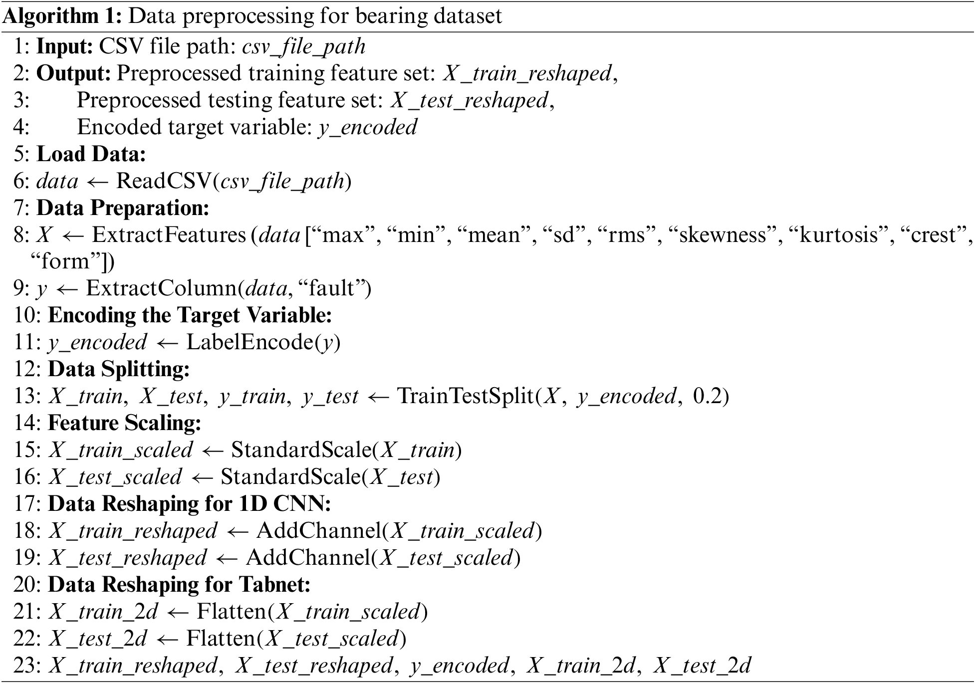
To ensure that the features are on a consistent scale and avoid issues related to different units or scales among attributes, the code standardizes the features using StandardScaler. Standardization transforms the features to have a mean of 0 and a standard deviation of 1, which is a common preprocessing step in machine learning. Finally, for those interested in applying a 1D CNN to this dataset, the code reshapes the data. This reshaping step adds an additional dimension (channel) to the feature data, which is often necessary for feeding sequential or time-series data into CNN architectures. In summary, this step prepares the dataset with specific columns related to bearing attributes for subsequent machine learning or deep learning tasks, including the potential use of a 1D CNN. Dataset pre-processing steps are also shown in Algorithm 1.

2.3 CNN and LSTM Model

Convolutional Neural Networks, known as simple computational models, represent the mammalian visual cortex. The CNNs are biologically inspired by feed-forward ANNs (Artificial Neural Networks). They are categorized into 1D, 2D, and 3D CNNs based on the problem the Model addresses. 2D and 3D CNNs focus on image and video data processing. 1D-CNNs process audio and text recognition (e.g., time series data). Among all CNN models, 1D-CNNs are considered the best tool for time series data processing, prediction, and identification [23,24]. They have gained popularity in bearing fault diagnosis due to their ability to extract valuable features from vibration signal data. These networks outperform other models because they can automate feature extraction, handle non-linearity, and provide fault localization. In this Model, the base layer (CNN layer) is a fundamental component that extracts all significant features from the given input data (vibration signal). The output of a convolutional layer in the CNN model can be represented by the following equation for a single feature map at position ‘(i, j)’:

O[i, j]=f(∑(I∗K)+b)(1)

where O[i, j] represents the output feature map value given at the (i, j) position in the CNN layers, I states the value of the input feature map, K is the convolutional kernel (filter) applied to the input, b is the bias term which introduces an offset in the feature map, f( ) is an activation function that helps the Model catching complex features or patterns by introducing non-linearity in the Model. Many activation functions are associated with CNNs like SoftMax, ReLU (Rectified Linear Unit), Tanh, and Sigmoid. For bearing fault diagnosis problems, the Sigmoid function is the best choice because it involves multiple classes. Each Convolutional layer of the CNN model is connected to the Pooling layer, which works by reducing the spatial dimensions present in the feature map while retaining the crucial information coming from the CNN layers. In the bearing fault diagnosis problem, max-pooling is the most commonly used pooling operation. The equation for the max-pooling operation is given as follows:

H[x, y]=max(M[x⋅s:x⋅s+(k, y)⋅s:y⋅s+k])(2)

where H[x, y] gives the feature map’s output value at a specific position (x, y) in the pooling layer, M is the input feature map from the previous layer, s is the step size, also known as stride at which the pooling window (typically a square window of size k × k) moves over the input feature map, k is the size of the pooling window (typically 2 × 2 or 3 × 3), max () is the max-pooling operation, which computes the maximum value within the pooling window. LSTM is a type of RNN layer (recurrent neural network) used in various sequential data processing tasks, including time series analysis and natural language processing.

LSTM layers are designed to capture long-range dependencies and handle data sequences by capturing important information from previous time steps with the help of a hidden state vector. A typical LSTM block consists of three gates. These gates include input, forget, and output gates. An activation function controls each gate to introduce non-linearity (the sigmoid function). These gates and a memory cell work together to control the movement of information within the LSTM cell. The input gate has the task of deciding what information given in the input data will be stored in the memory. Then, the other gate (forget gate) decides what information taken from the memory cell will be forgotten and retained. Lastly, the output gate decides what piece of information taken from the memory cell will be considered to compute the output. The equations for these three gates are given as follows:

xo=sigmoid(Qx⋅[kp−1, rp]+dx)(3)

yo=sigmoid(Qy⋅[kp−1, rp]+dy)(4)

zo=sigmoid(Qz⋅[kp−1, rp]+dz)(5)

kp=zo⋅tanh⁡(vp)(6)

2.4 FTCNNLSTM Architecture Overview

The proposed system aims to enhance bearing fault diagnosis in electric motor-driven systems by integrating two powerful neural network architectures: CNN-LSTM and TabNet. This integration, known as FRCNNLSTM, seeks to leverage the feature extraction capabilities of CNN-LSTM along with the interpretability and classification prowess of TabNet. By merging these architectures, the goal is to achieve higher accuracy and improved performance in diagnosing faults from time-series vibration data.

TabNet is a novel attention-based neural network architecture primarily used for tabular data analysis and classification tasks. It employs a structured attention mechanism to interpret and select important features while performing classification. The architecture consists of shared and attentional layers, utilizing Gated Linear Units (GLU) to effectively learn patterns and relationships within the data. TabNet’s key strength lies in its ability to offer interpretability alongside strong predictive performance.

The TabNet architecture comprises several key components: Shared and Attentional Layers: These layers, with specified dimensions (n_d and n_a), facilitate feature selection and learning important patterns within the data. Steps and Sparsity Control: TabNet operates through a series of steps (n_steps) while controlling sparsity using a relaxation parameter (gamma). GLU: These units, organized in independent and shared sets (n_independent and n_shared), enable effective feature selection and information flow within each step of the architecture. Batch Normalization: Utilizing batch normalization with a specified momentum value (momentum) aids in stabilizing and accelerating the training process.

In the FTCNN-LSTM architecture, TabNet is introduced as a classifier after the CNN-LSTM layers. This integration facilitates a comprehensive approach to fault diagnosis. The CNN-LSTM layers extract temporal patterns and dependencies from the time-series vibration data, while the TabNet classifier operates on the extracted features to enhance interpretability and perform the final classification.

The CNN-LSTM model can also handle complex temporal sequence problems by increasing the accuracy and efficiency of prediction. Thus, the combination of FTCNN-LSTM networks is a powerful architecture for time-series data (bearing fault diagnosis in electric motor-driven systems). This architecture leverages the feature extraction capabilities and the sequential modeling abilities. Fig. 2 represents the flow of the FTCNNLSTM architecture for CWRU bearing fault diagnosis data while Table 1 shows the architecture detail of the CNN-LSTM model:

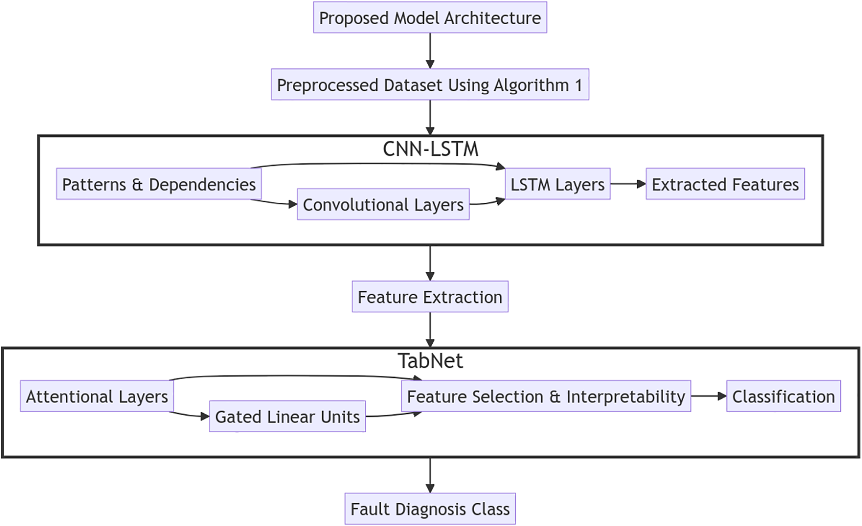
Figure 2: Architecture of FTCNNLSTM model

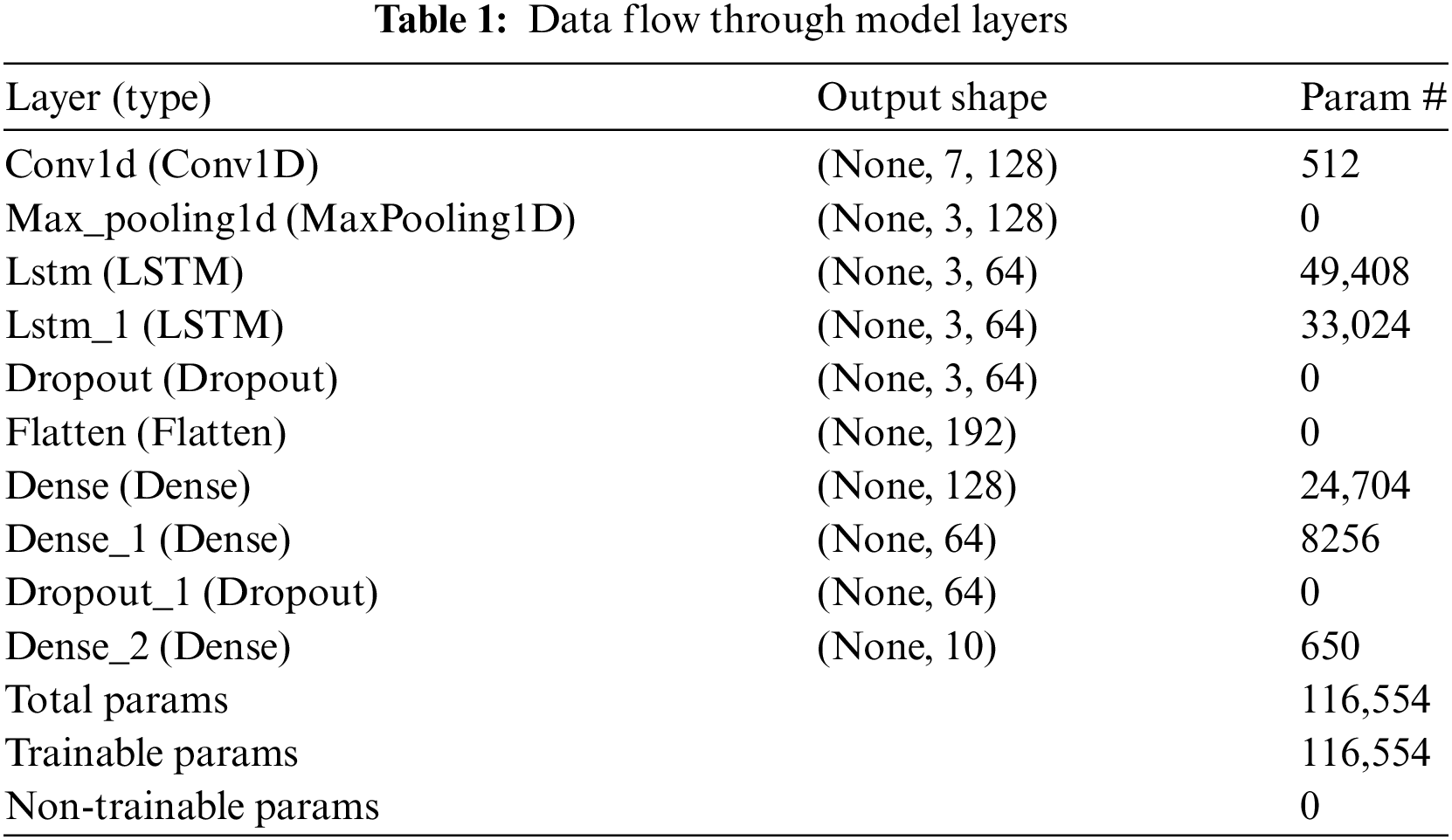
After loading the time series (vibrational signal), data from the CWRU dataset was segmented into fixed-length windows or sequences. The neural networks are efficiently trained over input data of consistent shape. The window size of 2048 samples was selected for segmenting the vibration signal data. For each window, the data was extracted as one sequence. These sequences served as individual data points for training the FTCNNLSTM model. After the segmentation task, another pre-processing technique, “Normalization,” was applied to the data. For the stability of the training process, the normalization technique helps in scaling each data point consistently. The equation for normalization is given as:

Nd=X−μσ(7)

Nd represents the normalized data, X represents the data, μ represents the mean of the data and σ denotes the standard deviation. For the prevention of data leakage, normalization was separately performed for training, validation, and testing datasets. The input layer of the FTCNN-LSTM model accepts the pre-processed (segmented and normalized) data. This layer is one of the CNN layers that will further extract features. A series of 1D-CNN layers captured local patterns by applying the learnable filters. The activation function sigmoid discussed previously is applied after each convolutional operation for introducing non-linearity and modeling the probability of class outcomes. The mathematical working of sigmoid is given as:

σ(i)=11+e−i(8)

where i is the input given to the sigmoid function, the max-pooling function is applied after the CNN layer. The significance and equation of this function are already discussed above. The hierarchal features are extracted by stacking multiple convolutional layers. The output of CNN layers is given as input to the LSTM layers. These LSTM layers then model the temporal dependencies. The LSTM cells were configured first with 64 and then 128 units. It is a crucial step in determining the Model’s capacity to capture temporal dependencies and patterns in the data. Dropout layers were further added to prevent overfitting. A dropout layer prevents the network from memorizing the training data by randomly dropping neurons during training. These layers support the network’s ability to learn more general and robust features. Mathematically, the dropout process can be expressed as:

bmi∼Bernoulli(dr)(9)

Oi=bmi⋅Ini1−dr(10)

bmi represents the binary mask of ith neuron, dr is the specified dropout rate. Ini is the given input to the ith neuron. Oi denotes the output of the ith neuron after applying the dropout. A dropout-trained model is more likely to generalize well to unseen data, making it suitable for tasks like bearing fault diagnosis, where robustness is essential.

Afterward, the output from the CNN-LSTM layers is fed into the TabNet classifier. Here, TabNet leverages its attention-based mechanism to discern essential features and provide interpretability while making the final predictions for bearing fault diagnosis.

Zo=S(D⋅Xo+b)(11)

where Zo is the output vector in the dense layer. S is the sigmoid function applied element-wise to the output. D represents the weight matrix. Xo is the input vector in the dense layer. b denotes the bias vector applying bias terms in each neuron of the dense layer. The network is analyzed using a categorical cross-entropy loss function for bearing fault diagnosis. This loss function is the most suitable function for classification problems like bearing fault diagnosis. The loss function indicates how dissimilar the true class labels are from the predicted class probabilities based on the difference between the two values. Mathematically, the categorical cross-entropy loss function is represented as follows:

L(Ytrue, Ypred)=−∑(Ytrue, i⋅log⁡(Ypred, i))(12)

Ytrue represents the true label of ground truth and Ypred represents the predicted probabilities. The Model is then trained and tested for various performance parameters, including accuracy, mean, standard deviation, kurtosis, skewness, etc. They deployed the fine-tuned Model for real-time or batch inference on new or unseen vibration data. Fine-tune hyperparameters such as the number of CNN and LSTM layers, filter sizes, units, dropout rates, and learning rates are applied to optimize model performance further. This chosen FTCNNLSTM model best targets the bearing fault diagnosis in electric motor-driven systems.

This integration of TabNet with CNN-LSTM in the FTCNNLSTM architecture combines the strengths of both models, aiming for superior accuracy and interpretability in diagnosing bearing faults from complex time-series data. It has achieved higher accuracy and performance than other previous models.

2.5 CNN-LSTM-Random Forest Model

Another algorithm using the ensembled approach was implemented on the CWRU bearing fault data. This Model combined CNN-LSTM with a random forest algorithm consisting of 100 individual decision trees known as estimators. A meta-classifier named Random_Forest_classifier was used to combine the outputs of all base models (CNN-LSTM-RF) and make the final prediction. Stacking_Classifier and Estimators are the two parameters taken from Scikit Learn for building the stacking ensemble model and generating the predictions from the base models. The simulation consists of 100 estimators with a random state of 42. Further, the stacking ensemble model’s output was given by the final estimator parameter of the meta-classifier. The Model was trained on 2300 instances and tested on 460 data points using the ‘fit’ method. The Model’s fitting equation is given as.

2.6 CNN-LSTM Model with Gradient Boosting

Gradient Boosting is an ensemble learning method that combines the predictions of multiple automated machine learning models to create a stronger, more accurate model. The core idea behind Gradient Boosting is to train a sequence of weak learners, where each new learner corrects the errors made by the previous one. This study combined CNN-LSTM with a gradient boosting algorithm (an ensembled approach) to detect bearing faults in electric motor-driven systems. In this Model, the meta-classifier is called Gradient_Boosting_classifier, which will combine the outputs generated from the base models being CNN, LSTM, and GB (Gradient Boosting) and give final predictions. The same parameters from Scikit Learn used in the CNN-LSTM-RF model were implemented in this Model. The above models were trained and tested on the same number of data points (460 for testing and 2300 for training).

3  Results

In this study, the proposed FTCNNLSTM has proven to be an efficient model for detecting bearing faults in electric motor-driven systems. To further explain the performance and efficiency of the FTCNNLSTM model, four other state-of-the-art algorithms were implemented to the CWRU bearing faults dataset and compared with the results. These four models include CNN, LSTM, CNN-LSTM with gradient boosting, and CNN-LSTM with random forest. The algorithms’ performance was analyzed and interpreted based on a few parameters. These parameters included the accuracy and loss of the models, the Receiver Operating Characteristic (ROC) curve of the models, the confusion matrix of the models, stats such as precision, F1-score, support, and the recall score of the models. This section presented a detailed comparison of the results focused on the FTCNNLSTM model being the most efficient and accurate algorithm for bearing fault diagnosis in electric motor-driven systems. Each parameter with results of all the models is presented below.

3.1 Accuracy and Loss Graph

The accuracy graph shows how the Model’s performance evolves as it learns from the training data. Initially, accuracy might be low, reflecting that the Model is making random predictions. Table 2 shows the accuracy and loss values for all CNN, LSTM, and FTCNNLSTM models. Over time, accuracy typically increases as the Model learns to make better predictions and generalize well on unseen complex data. If the Model is achieving high accuracy in training and validation data, it is working well and preventing over-fitting. The loss graph illustrates how the Model’s errors decrease as it learns. A high initial loss is expected but should decrease over time, reflecting improved predictions. Fig. 3 shows the Accuracy and loss graphs of all the models except an ensemble approach such as CNN-LSTM with gradient boosting and CNN-LSTM applied in correspondence to the random forest.

•   CNN Model: The initial accuracy was 0, which is typically expected as the Model has not learned anything yet, and throughout 80 epochs, both the training and validation accuracies improved. At 100 epochs, it reached 0.93% for both training and validation. This is a positive sign as it indicates that the Model could generalize well, performing almost equally on the data it was trained on and unseen data. The Model’s loss for the training data started at a peak of five and reached close to 0.15% after 100 epochs. For the validation data, the loss graph started at a value of 2 and reached close to 0.1 after 100 epochs. This is a sign that the Model effectively learned from the training data and could generalize well to data it had not seen during training. Overall, the Model was preventing overfitting.

•   LSTM Model: The initial accuracy was close to 0.1 because the Model had not learned anything at the start, but over 40 epochs, the accuracies increased exponentially. At 40 epochs, it reached 94% for training and validation, indicating that the Model is learning the features effectively and can generalize well on the unseen data. The Model’s loss for the training data started at a peak value of 2.25 and reached close to 0.25 after 40 epochs. For the validation data, the loss graph started at a value of 1.78 and reached close to 0.23 after 40 epochs. This shows that the Model was correctly predicting the faults in all classes and preventing over-fitting by learning the complex features and recognizing unseen data. Based on Accuracy and loss graphs, FTCNN-LSTM achieved the highest accuracy of 94% and outperformed other models.

•   FTCNNLSTM Model: The initial accuracy for training data and validation data was close to 0.2. At 100 epochs, it reached 0.96 for training and validation, indicating that the Model is learning the features effectively and performing almost equally on both the data it was trained on and unseen data. The Model’s loss for the training data started at a peak of 2 and reached close to 0.1 after 100 epochs. For the validation data, the loss graph started at a value of 1.6 and reached close to 0.1 after 100 epochs. It indicates that the Model performed efficiently and predicted the unseen data correctly.

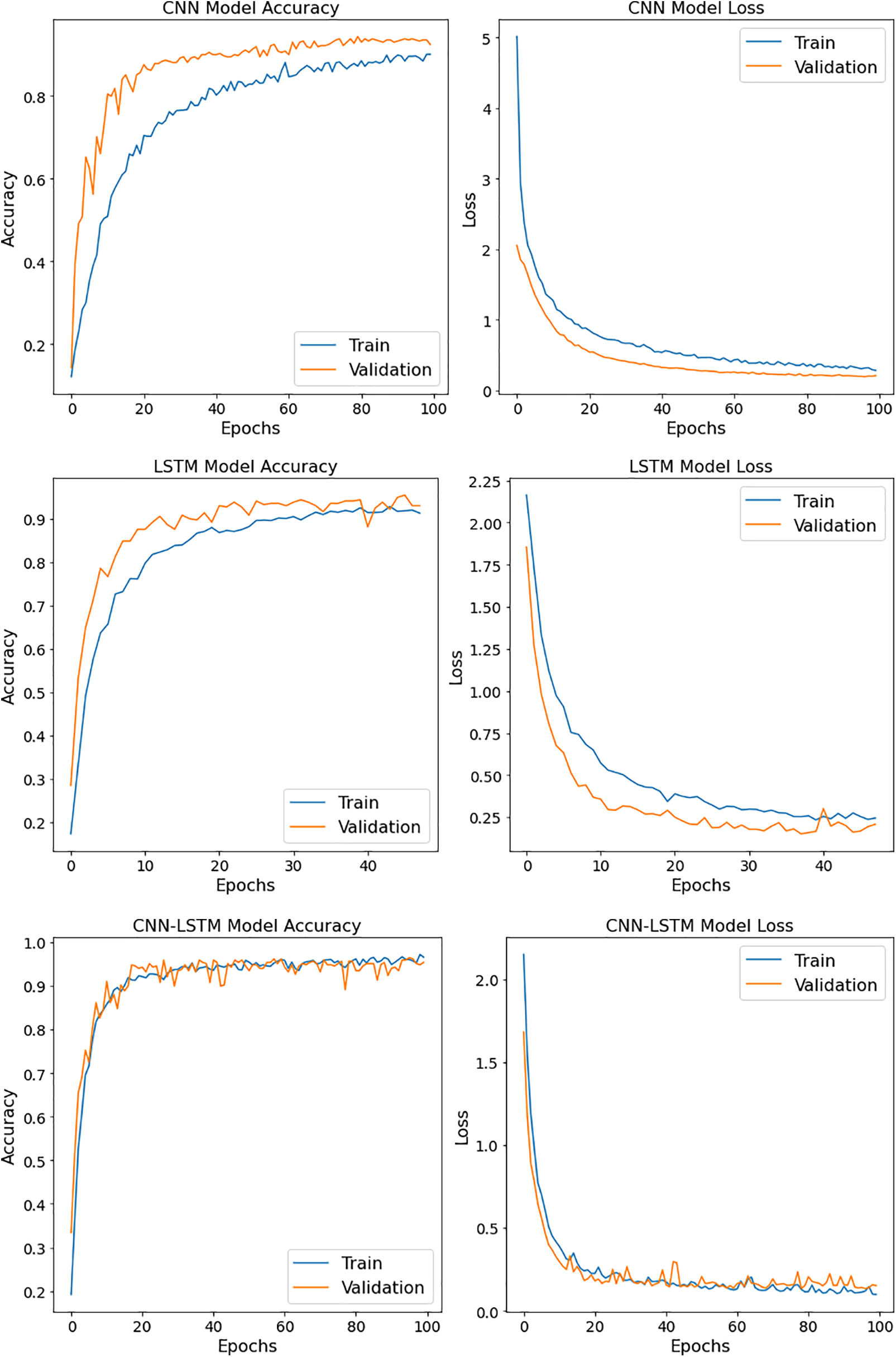
Figure 3: Accuracy and loss graphs of CNN, LSTM, and FTCNN-LSTM models

3.2 ROC Curve and AUC

The ROC curve graph for all models in Fig. 4 represents the Model’s predicted true positive rate on the x-axis and false positive rate on the y-axis. ROC AUC (Area under the curve) for all models, as shown in Fig. 4, quantifies the overall ability of the Model to discriminate between the positive and negative classes across various classification thresholds.

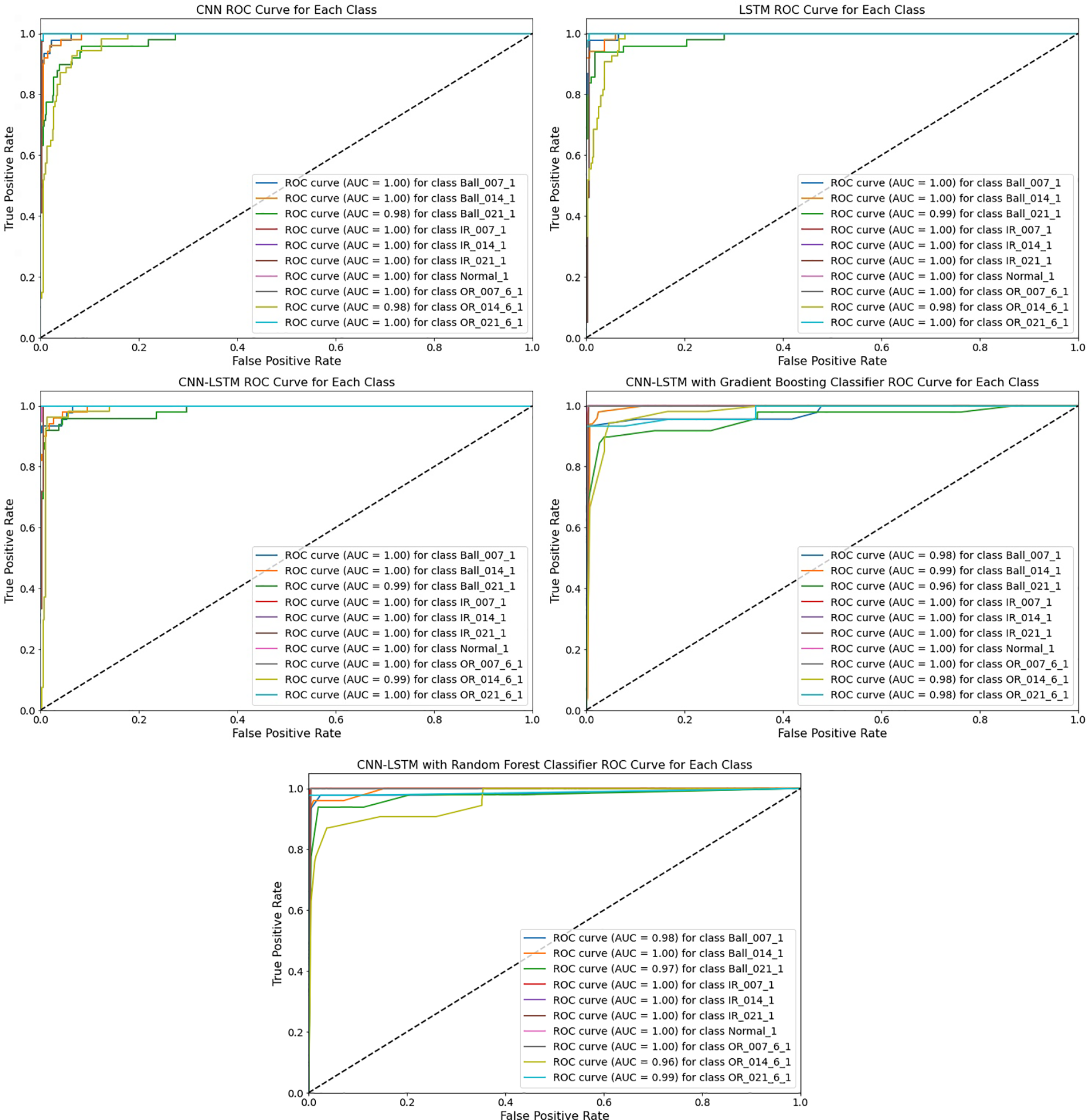
Figure 4: ROC curve graph for CNN, LSTM, FTCNNLSTM, CNN-LSTM with gradient boosting, and CNN-LSTM with random forest models

3.3 Confusion Matrix

Confusion matrix is a parameter in the machine learning algorithms that is used to evaluate the performance of an algorithm by providing a detailed breakdown of its predictions compared to the actual ground truth. This parameter shows the number of correct and incorrect predictions made by the Model for each class. The key components of the confusion matrix are:

1.    True Positives (TrPo): These are the positive instances or data points correctly predicted by the Model for all the classes.

2.    True Negatives (TrNe): These are the negative instances or data points correctly predicted by the Model for all the given classes.

3.    False Positives (FaPo): These are the negative instances that were incorrectly predicted and shown to be positive by the Model within all the classes.

4.    False Negatives (FaNe): These are the positive data points or instances that were shown as negatives by the Model within all of the given classes. The confusion matrix for all implemented models is shown in Fig. 5.

•   CNN Model: The Model has predicted almost 9 out of 10 classes correctly. The major issue was seen in the outer race class recorded at 6 o’clock with 0.014 diameter as Model misclassified twelve OR_014_6_1 fault as Ball_021_1, seven as Ball_014_1, and three as Ball_007_1. The Model also incorrectly predicted two OR_021_6_1 as Ball_014_1 and IR_007_1, respectively. It can be seen that the Model incorrectly predicted two faults in each Ball_007_1, Ball_014_1, and Ball_021_1 class as OR_014_6_1.

•   LSTM Model: Overall, the confusion matrix interprets that the Model performed well. The model misclassified OR_014_6_1 fault as three Ball_007_1, three Ball_014_1, and one Ball_021_1 fault. The Model also incorrectly predicted one Ball_014_1 fault as Normal machine, two Ball_021_1 fault as IR_021_1, and one OR_021_6_1 fault as IR_007_1. It can be seen that the Model incorrectly predicted three faults in Ball_007_1, two faults in Ball_014_1, and seven faults in Ball_021_1 class as OR_014_6_1.

•   CNN-LSTM with gradient boosting Model: This model was able to identify most of the bearing fault classes correctly. There were some errors as the model misclassified one Ball_007_1 fault as Ball_014_1, two Ball_007_1 fault as OR_014_6_1, one Ball_014_1 fault as OR_014_6_1, twelve Ball_021_1 fault as OR_014_6_1, two Ball_021_1 fault as Ball_007_1, and one Ball_021_1 fault as Ball_014_1, two Ball_021_1 fault as IR_021_1, one normal motor as Ball_014_1 fault. The Model also incorrectly identified one OR_014_6_1 fault as Ball_007_1 and five OR_014_6_1 fault as Ball_014_1, two OR_021_6_1 fault as Ball_014_1, and one OR_021_6_1 fault as IR_007_1 fault.

•   CNN-LSTM with random forest Model: The confusion matrix of the CNN-LSTM-RF model shows that the Model was able to predict maximum fault classes correctly. However, nine, four, and seven OR_014_6_1 fault as Ball_007_1, Ball_014_1, and Ball_021_1, respectively. It misclassified two Ball_014_1 and two Ball_021_1 faults as IR_021_1 and OR_014_6_1 faults, respectively. The Model also incorrectly predicted one Ball_007_1 fault as Ball_021_1 and one OR_014_6_1 fault as IR_007_1.

•   FTCNN-LSTM Model: The FTCNN-LSTM Model outperformed all of the other approaches. This Model achieved the highest accuracy as it correctly identified maximum fault classes. However, the Model needed to correct a few while classifying the fault types. The matrix shows that the Model incorrectly identified one Ball_007_1 fault as Ball_021_1 fault, one Ball_014_1 fault as Ball_021_1, two Ball_007_1 and five Ball_014_1 fault as OR_014_6_1 fault. The Model also misclassified two Ball_021_1 fault as Ball_007_1, two Ball_021_1 fault as IR_021_1, one Ball_014_1 fault as Normal/healthy motor, and two OR_014_6_1 fault as Ball_014_1 and Ball_021_1 fault.

Figure 5: Confusion matrix for CNN, LSTM, FTCNN-LSTM, CNN-LSTM with gradient boosting, and CNN-LSTM with random forest models

3.4 Classification Report

The classification report for all implemented models was presented, as shown in Fig. 6. This report consists of various performance metrics of the algorithm. This report helps in assessing the Model’s strengths and weaknesses. The metrics included in the study are:

1.    Accuracy (Ac): The segment of correctly classified instances (TrPo + TrNe) out of the total data points.

2.    Precision (Pr): The number of positive instances correctly predicted as positives (TrPo/(TrPo + FaPo)).

3.    Recall (Rc): The proportion of true positives out of all actual positive instances (TrPo/(TrPo + FaNe)).

4.    F1-score (Fs): The harmonic mean of Pr and Rc scores balances the two metrics.

5.    Support: This parameter shows the number of instances or data points considered for the training and validation process.

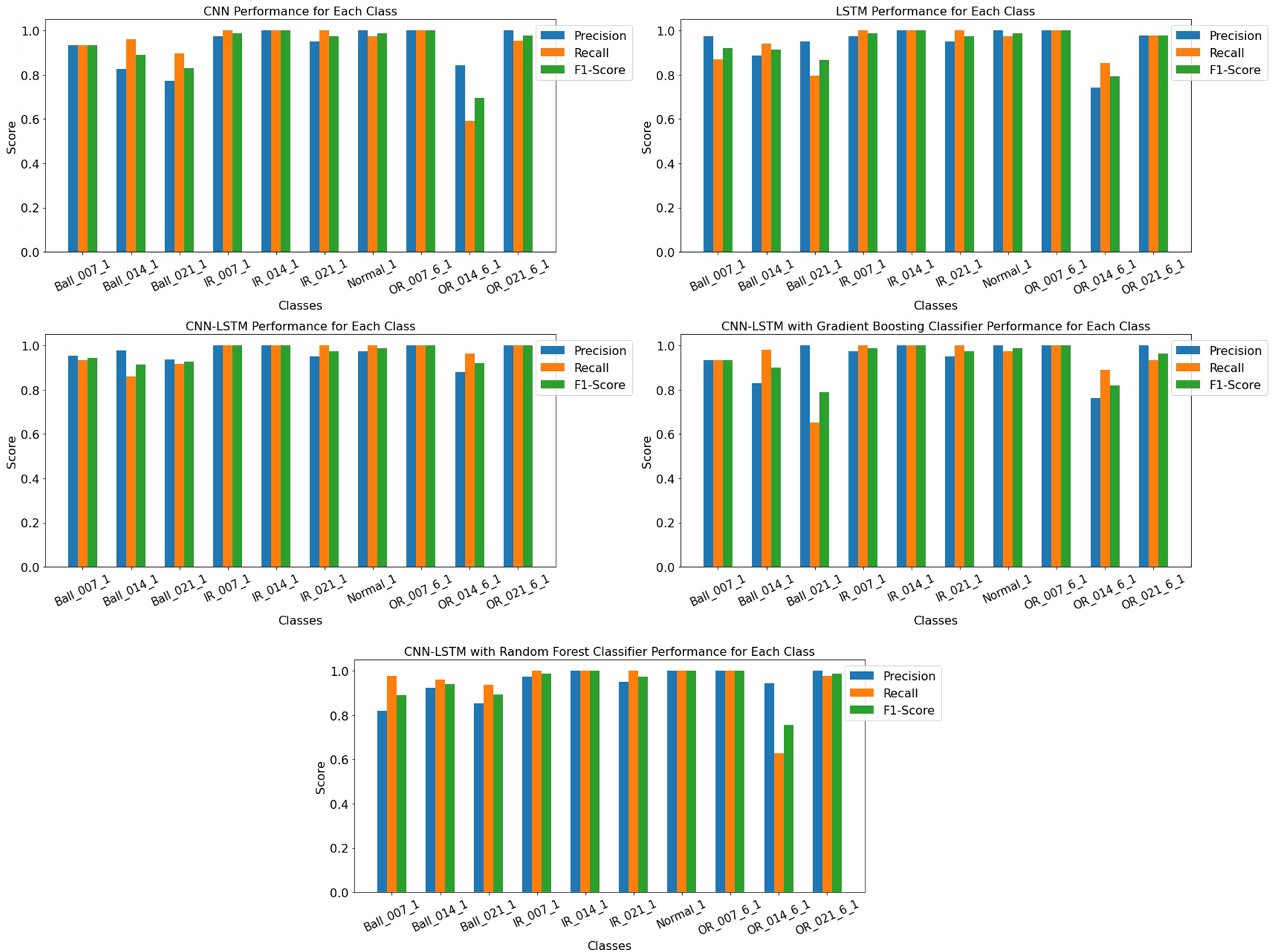
Figure 6: Precision, F1-score, and recall score graphs for each model

The classification report shows the Pr, Ac, Rc, and Fs of each model concerning each class in Table 3. The CNN model achieved an overall accuracy of 92% with a support of 460 instances. The Model achieved the highest scores for Pr (1.00), Fs (1.00), and Rc (1.00) for OR_007_6_1, and IR_014_1 fault class and achieved 1.00 Pr score, 0.97 recall and 0.99 Fs for normal class. The CNN-LSTM model with gradient boosting achieved an overall accuracy of 93% with a support of 460 instances. The Model achieved the highest scores for Pr (1.00), Fs (1.00), and recall probability (1.00) for IR_014_1 and OR_007_6_1 fault class and achieved a 1.00 precision score, 0.97 Rc probability and 0.99 Fs for normal class.

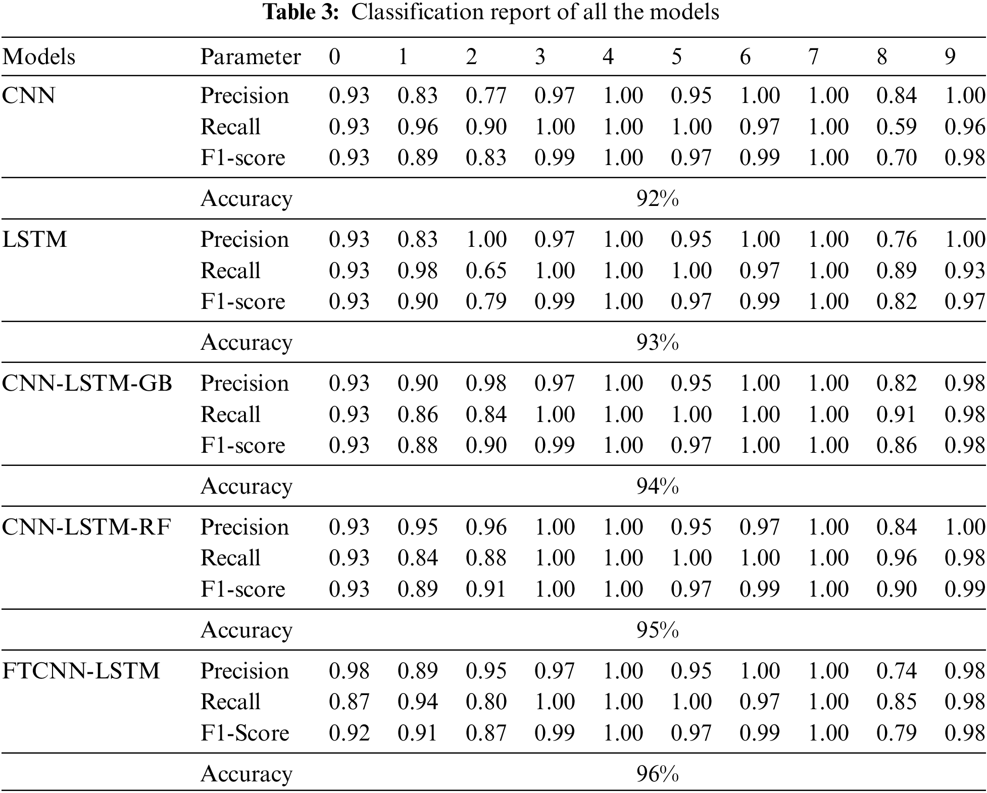
The LSTM model achieved an overall accuracy of 93% with a support of 460 instances. The Model achieved the highest scores for Pr (1.00), Fs (1.00), and Rc (1.00) for IR_014_1 and OR_007_6_1 fault class and achieved 1.00 Pr, 0.97 Rc and 0.99 Fs for normal_1 class. The CNN-LSTM model with gradient boosting achieved an overall accuracy of 95% with a support of 460 instances. The Model achieved the highest scores for Pr (1.00), Fs (1.00), and recall probability (1.00) for IR_014_1, Normal_1, and OR_007_1 class. The proposed FTCNN-LSTM model achieved an overall accuracy of 96% with a support of 460 instances. The Model achieved the highest scores for precision (1.00), Fs (1.00), and Rc probability (1.00) for OR_007_6_1, IR_007_1, and IR_014_1 fault class and achieved 0.97 Pr score, 1.00 recall probability, and 0.99 Fs for normal electric motors. The Pr, Fs, and Rc charts are shown in Fig. 6.

3.5 Comparison of FTCNN-LSTM Model with Other Approaches

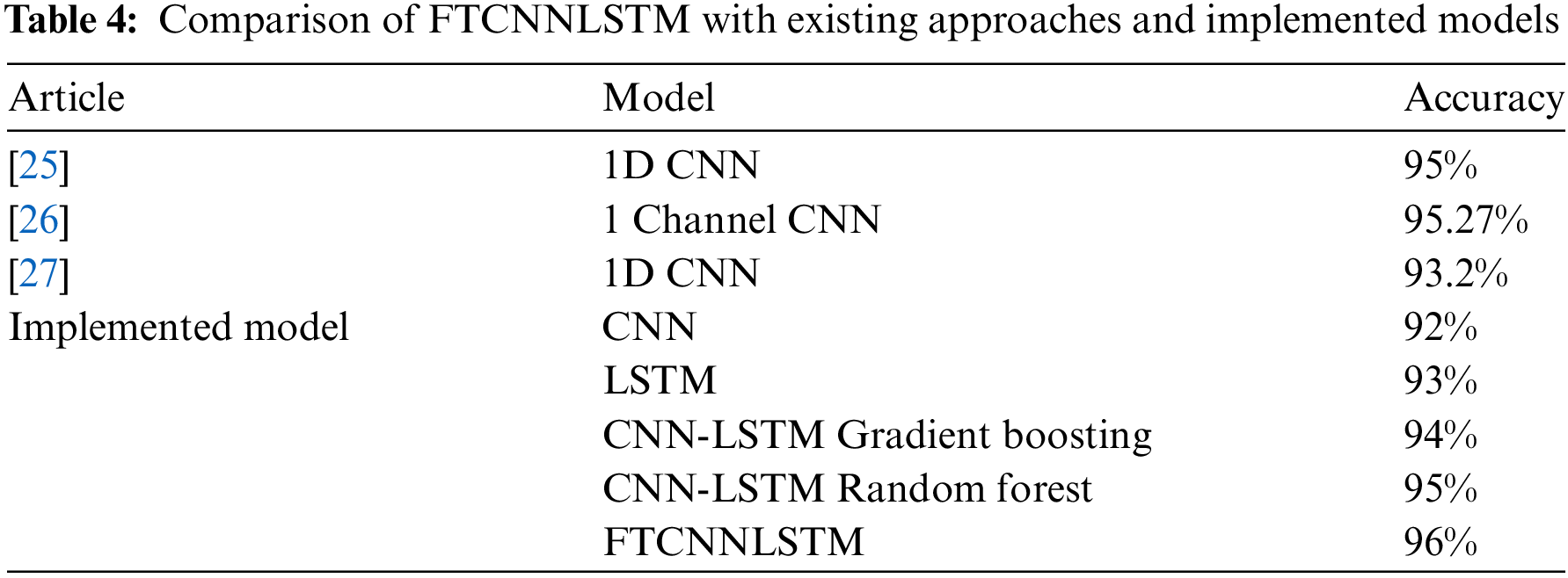
As stated in the previous sections, four approaches were implemented to evaluate and compare the performance with the proposed FTCNNLSTM model. Table 4 shows the comparison of existing approaches to the proposed FTCNNLSTM model. Some other previously published algorithms were also studied and compared with the proposed approach. One of these algorithms includes a 1D CNN model with linear embedding as a data pre-processing technique [25]. The model claimed to achieve an accuracy of 95% for a very small sample size and ten classes of bearing faults. Another approach, 1 channel CNN, was implemented on the CWRU bearing fault dataset, and it achieved 95.27% accuracy [26]. 1D CNN model was also used to detect bearing faults in electric motor-driven systems [27]. This approach used filtering decimation and normalization data pre-processing techniques. The model achieved 93.2% accuracy on the CWRU dataset by experimenting with only six classes. FTCNNLSTM combined the potential of CNNs and LSTM models, and by fine-tuning the entire algorithm achieved 96% accuracy by working on ten classes of bearing faults. This proves the FTCNNLSTM model can efficiently detect bearing faults in electric motor-driven systems.

4  Discussion

Electric motor-driven systems play a crucial role in the manufacturing of industrial machinery. Despite their importance, machines and electronics driven by electric motors are susceptible to failures and faults. Early fault diagnosis is highly important for preventing economic losses and enhancing machines and equipment’s reliability and performance. In this study, a fine-tuned CNN-LSTM model was implemented on the CWRU bearing faults diagnosis dataset. Combining CNN-LSTM with Tabnet networks and applying fine-tuning to the Model is a powerful architecture for bearing fault diagnosis in electric motor-driven systems. This architecture leverages the feature extraction capabilities of CNNs and the sequential modeling abilities of LSTMs. The result section has proven the capability and efficiency of the FTCNN-LSTM model in detecting bearing faults within electric motors.

All the models performed well on bearing fault classes, but the proposed FTCNN-LSTM model outperformed all these algorithms by achieving the highest performance scores. All of the performance metrics, including Pr, Fs, Ac, and Rc scores, showed that all the models could correctly predict the bearing faults in motors. For all the classes, these scores ranged from 54% to 100%. For the FTCNN-LSTM model, these performance scores ranged from 84% to 100% with an overall accuracy of 96%. The Pr, Fs, and Rc scores were consistent for most classes. These matrices show that all models could correctly classify maximum bearing faults within electric motors. FTCNNLSTM had gone through effective pre-processing techniques such as normalization and applied activation functions and had been fine-tuned. This Model achieved the highest scores, which clearly shows that the Model is learning well and efficiently dealing with unseen complex data.

A confusion matrix for all the models was generated. This matrix demonstrated that most models correctly classified the bearing fault classes. However, on the time-series vibrational data, FTCNNLSTM also faced some challenges. As explained above in the detailed overview of confusion matrix results, the models needed to be more accurate in classifying misclassified fault classes. OR_014_6_1 was misclassified in almost all of the models. FTCNNLSTM also showed the most satisfying results in the confusion matrix. Unlike other models that misclassified nearly 25 instances among all of the classes, the FTCNNLSTM Model misclassified 16 instances with a maximum of 5 consecutive Ball_014_1 faults as OR_014_6_1. The models were further compared based on their strengths and weaknesses. Each Model has some drawbacks based on the performance results. For instance, the CNN-LSTM with a combined random forest model applied an ensemble approach but could not correctly classify the OR_014_6_1 bearing faults. CNN-LSTM with gradient boosting, also an ensembled approach, faced difficulty correctly classifying Ball_021_1 bearing faults. Based on the accuracy scores, all of the models were compared with some existing approaches given in the literature.

The implemented models, CNN, achieved 92% accuracy, LSTM, achieved 93% of Ac score, and CNN-LSTM, ensembled with gradient boosting, got 94% accuracy. The other method, CNN-LSTM combined with random forest, achieved a 95% Ac score. FTCNNLSTM combined the potential of CNNs-LSTM with Tabnet models achieving 96% accuracy by working on ten classes of bearing faults. This proves the FTCNNLSTM model can efficiently detect bearing faults in electric motor-driven systems.

5  Conclusion

This study presents the FTCNNLSTM model, an advanced and comprehensive approach for bearing fault detection and diagnosis in electric motor-driven systems. FTCNNLSTM synergizes CNNs for robust feature extraction and the sequential modeling capabilities of LSTM networks, providing an efficient and accurate solution for this critical task. In assessing the FTCNNLSTM model’s performance, a rigorous comparative analysis against established methodologies, including CNN, LSTM, CNN-LSTM with gradient boosting, CNN-LSTM combined with random forest, SVM, DNN, and a deep kernel-based learning approach. Notably, the FTCNNLSTM model, augmented with the interpretative prowess of TabNet, surpassed these alternatives, showcasing superior accuracy and fault classification capabilities. Leveraging the CWRU bearing fault diagnosis dataset, featuring 10 classes representing various motor faults, the comprehensive evaluation spanned multiple performance parameters. These assessments, incorporating classification reports, confusion matrices, accuracy metrics, and loss graphs, consistently reaffirmed the FTCNNLSTM model’s effectiveness in fault diagnosis. Ultimately, the FTCNNLSTM model demonstrated exceptional performance, achieving an outstanding accuracy rate of 96%. The FTCNNLSTM model, while highly accurate, faces challenges in computational complexity and data requirements. Its performance on the CWRU dataset is promising, but further validation is needed. Future research should focus on optimizing efficiency, expanding validation across diverse datasets, exploring integration with advanced architectures like Transformers, extending to quality-level prediction tasks, and enhancing model interpretability. These efforts aim to improve the model’s applicability and acceptance in industrial settings.

Acknowledgement: The authors gratefully acknowledge the funding support by King Abdulaziz University, Deanship of Scientific by King Abdulaziz University, Deanship of Scientific Research, Jeddah, Saudi Arabia under grant no. (GWV-8053-2022).

Funding Statement: This study was supported by King Abdulaziz University, Deanship of Scientific Research, Jeddah, Saudi Arabia under grant no. (GWV-8053-2022).

Author Contributions: The authors confirm contribution to the paper as follows: study conception and design: Alaa U. Khawaja, Ahmad Shaf, Tariq Ali; data collection: Ahmad Shaf, Aqib Rehman Pirzada, Muhammad Irfan; analysis and interpretation of results: Alaa U. Khawaja, Faisal Al Thobiani, Muhammad Irfan, Aqib Rehman Pirzada; draft manuscript preparation: Ahmad Shaf, Unza Shahkeel, Tariq Ali. All authors reviewed the results and approved the final version of the manuscript.

Availability of Data and Materials: Dataset can be downloaded from the given link: https://mb.uni-paderborn.de/en/kat/main-research/datacenter/bearing-datacenter/data-sets-and-download (accessed on 30 July 2024). Code can be shared upon certain request to the corresponding author.

Conflicts of Interest: The authors declare that they have no conflicts of interest to report regarding the present study.

References

1. Xu M, Lv X, Li C, Zhang F, Liu C, Liu M, et al. An EHV transformer fault diagnosis method based on acoustic perception and sparse autoencoder-BNCNN. J Phys: Conf Series. 2023;2495:12019. doi:10.1088/1742-6596/2495/1/012019. [Google Scholar] [CrossRef]

2. Liu R, Yang B, Zio E, Chen X. Artificial intelligence for fault diagnosis of rotating machinery: a review. Mech Syst Signal Process. 2018;108:33–47. doi:10.1016/j.ymssp.2018.02.016. [Google Scholar] [CrossRef]

3. Li Y, Xu M, Wei Y, Huang W. Health condition monitoring and early fault diagnosis of bearings using SDF and intrinsic characteristic-scale decomposition. IEEE Trans Instrum Meas. 2016;65(9):2174–89. doi:10.1109/TIM.2016.2564078. [Google Scholar] [CrossRef]

4. Riera-Guasp M, Antonino-Daviu JA, Capolino GA. Advances in electrical machine, power electronic, and drive condition monitoring and fault detection: state of the art. IEEE Trans Ind Electron. 2014;62(3):1746–59. doi:10.1109/TIE.2014.2375853. [Google Scholar] [CrossRef]

5. Ágoston K. Fault detection of the electrical motors based on vibration analysis. Proc Technol. 2015;19:547–53. doi:10.1016/j.protcy.2015.02.078. [Google Scholar] [CrossRef]

6. Mehala N, Dahiya R. Motor current signature analysis and its applications in induction motor fault diagnosis. Int J Sys App, Eng Dev. 2007;2(1):29–35. [Google Scholar]

7. Singh G, Kumar TA, Naikan V. Fault diagnosis of induction motor cooling system using infrared thermography. In: 2016 IEEE 6th International Conference on Power Systems (ICPS), 2016; New Delhi, India: IEEE; p. 1–4. doi:10.1109/ICPES.2016.7584040. [Google Scholar] [CrossRef]

8. Pham MT, Kim JM, Kim CH. Intelligent fault diagnosis method using acoustic emission signals for bearings under complex working conditions. Appl Sci. 2020;10(20):7068. doi:10.3390/app10207068. [Google Scholar] [CrossRef]

9. Wu JD, Liu CH. An expert system for fault diagnosis in internal combustion engines using wavelet packet transform and neural network. Expert Syst Appl. 2009;36(3):4278–86. doi:10.1016/j.eswa.2008.03.008. [Google Scholar] [CrossRef]

10. Gangsar P, Tiwari R. A support vector machine based fault diagnostics of Induction motors for practical situation of multi-sensor limited data case. Measurement. 2019;135:694–711. doi:10.1016/j.measurement.2018.12.011. [Google Scholar] [CrossRef]

11. Nguyen NT, Nguyen HP. Fault diagnosis of voltage source inverter for induction motor drives using decision tree. In: 9th International Conference on Robotic, Vision, Signal Processing and Power Applications: Empowering Research and Innovation, 2016; Singapore: Springer; p. 819–26. doi:10.1007/978-981-10-1721-6_88. [Google Scholar] [CrossRef]

12. Quiroz JC, Mariun N, Mehrjou MR, Izadi M, Misron N, Radzi MAM. Fault detection of broken rotor bar in LS-PMSM using random forests. Measurement. 2018;116:273–80. doi:10.1016/j.measurement.2017.11.004. [Google Scholar] [CrossRef]

13. Samanta S, Bera J, Sarkar G. KNN based fault diagnosis system for induction motor. In: 2016 2nd International Conference on Control, Instrumentation, Energy & Communication (CIEC), 2016; Kolkata, India: IEEE; p. 304–8. doi:10.1109/CIEC.2016.7513791. [Google Scholar] [CrossRef]

14. Pandarakone SE, Gunasekaran S, Mizuno Y, Nakamura H. Application of naive bayes classifier theorem in detecting induction motor bearing failure. In: 2018 XIII International Conference on Electrical Machines (ICEM), 2018; Alexandroupoli, Greece: IEEE; p. 1761–7. doi:10.1109/ICELMACH.2018.8506836. [Google Scholar] [CrossRef]

15. Yoo YJ. Fault detection of induction motor using fast Fourier transform with feature selection via principal component analysis. Int J Precis Eng Manuf. 2019;20(9):1543–52. doi:10.1007/s12541-019-00176-z. [Google Scholar] [CrossRef]

16. Ribeiro Junior RF, dos Santos Areias IA, Campos MM, Teixeira CE, da Silva LEB, Gomes GF. Fault detection and diagnosis in electric motors using convolution neural network and short-time fourier transform. J Vib Eng Technol. 2022;10(7):2531–42. doi:10.1007/s42417-022-00501-3. [Google Scholar] [CrossRef]

17. Principi E, Rossetti D, Squartini S, Piazza F. Unsupervised electric motor fault detection by using deep autoencoders. IEEE/CAA J Autom Sin. 2019;6(2):441–51. doi:10.1109/JAS.2019.1911393. [Google Scholar] [CrossRef]

18. Sabir R, Rosato D, Hartmann S, Guehmann C. LSTM based bearing fault diagnosis of electrical machines using motor current signal. In: 2019 18th IEEE International Conference on Machine Learning and Applications (ICMLA), 2019; Boca Raton, FL, USA: IEEE; p. 613–8. doi:10.1109/ICMLA.2019.00113. [Google Scholar] [CrossRef]

19. Liu H, Zhou J, Zheng Y, Jiang W, Zhang Y. Fault diagnosis of rolling bearings with recurrent neural network-based autoencoders. ISA Trans. 2018;77:167–78. doi:10.1016/j.isatra.2018.04.005. [Google Scholar] [PubMed] [CrossRef]

20. Liu W, Zhao C. ETM: effective tuning method based on multi-objective and knowledge transfer in image recognition. IEEE Access. 2021;9:47216–29. doi:10.1109/ACCESS.2021.3062366. [Google Scholar] [CrossRef]

21. Samek W, Montavon G, Lapuschkin S, Anders CJ, Müller KR. Explaining deep neural networks and beyond: a review of methods and applications. Proc IEEE. 2021;109(3):247–78. doi:10.1109/JPROC.2021.3060483. [Google Scholar] [CrossRef]

22. Li X, Zhang W, Ma H, Luo Z, Li X. Domain generalization in rotating machinery fault diagnostics using deep neural networks. Neurocomputing. 2020;403:409–20. doi:10.1016/j.neucom.2020.05.014. [Google Scholar] [CrossRef]

23. Kiranyaz S, Avci O, Abdeljaber O, Ince T, Gabbouj M, Inman DJ. 1D convolutional neural networks and applications: a survey. Mech Syst Signal Process. 2021;151:107398. doi:10.1016/j.ymssp.2020.107398. [Google Scholar] [CrossRef]

24. Khorram A, Khalooei M, Rezghi M. End-to-end CNN + LSTM deep learning approach for bearing fault diagnosis. Appl Intell. 2021;51(2):736–51. doi:10.1007/s10489-020-01859-1. [Google Scholar] [CrossRef]

25. AlThobiani F. A novel framework for robust bearing fault diagnosis: preprocessing, model selection, and performance evaluation. IEEE Access. 2024;12:59018–36. doi:10.1109/ACCESS.2024.3390234. [Google Scholar] [CrossRef]

26. Magar R, Ghule L, Li J, Zhao Y, Farimani AB. FaultNet: a deep convolutional neural network for bearing fault classification. IEEE Access. 2021;9:25189–99. doi:10.1109/ACCESS.2021.3056944. [Google Scholar] [CrossRef]

27. Eren L, Ince T, Kiranyaz S. A generic intelligent bearing fault diagnosis system using compact adaptive 1D CNN classifier. J Signal Process Syst. 2019;91(2):179–89. doi:10.1007/s11265-018-1378-3. [Google Scholar] [CrossRef]