A New Isogeometric Finite Element Method for Analyzing Structures

1  Introduction

High-performance finite element analysis (FEA) is a key research area within finite element methods (FEM). Many researchers have proposed elements aimed at overcoming the limitations and deficiencies of conventional FEM [1], such as non-conforming elements and extended finite element methods [2,3]. Xiang et al. [4,5] developed the wavelet finite element method and achieved excellent results in plate and shell analysis. Engel et al. [6] introduced the continuous/discontinuous Galerkin method, which relaxes the requirements of continuity between elements. This method allows for the implementation of non-rotational FEM in the thin bending theory. Romero [7] developed a new interpolation strategy and integrated it with FEM to analyze nonlinear bar models. Taylor et al. [8] proposed a three-field variational FEM for Euler and Timoshenko beams based on the Hu–Washizu principal extension, allowing for inelastic material behavior. Santos [9,10] constructed a force-based finite element formula using the complementary energy method for nonlinear Euler-Bernoulli beam structures. These formulations generate a direct and consistent variational formula, thereby avoiding locking effects. Mohri et al. [11] established a model for the behavior of thin-walled beams with open cross-sections, considering large torsion, linear, and nonlinear warping. In complex rotor systems, Xiang et al. [12] studied the construction of wavelet-based rotating shaft elements and successfully calculated the parameters of the dynamic model. Recently, graphics processing units have been introduced into FEM to improve computational efficiency and accelerate mesh optimization [13,14]. Lu et al. [15] proposed a method that combined reduced-order machine learning methods with finite element methods, which can reduce the size of the model and handle high-dimensional problems. These methods have improved the performance of elements to varying degrees. However, FEA and computer-aided design (CAD) are often separated, requiring expensive mesh generation work to convert geometric models into numerical models.

Isogeometric analysis (IGA), pioneered by Hughes et al. [16], utilizes non-uniform rational B-spline (NURBS) functions in CAD to represent geometry and approximate field variables in numerical models, bridging the gap between geometric and numerical modeling. IGA offers several advantages: (1) No need for mesh generation; (2) Geometric accuracy is maintained with any mesh refinement stage. (3) IGA incorporates the most common FE programs, contributing to its increasing acceptance and application [17–19]. The high-order continuity of B-splines and NURBS makes them widely used in IGA. For detailed information on them, please refer to [20]. The advantages of IGA have attracted extensive research. Combining IGA with other numerical methods such as the meshless method and boundary element method is currently one of the research hotspots [21,22]. Studies have shown that replacing NURBS with other spline functions can improve the mesh quality of IGA [23,24]. IGA has also been extended to artificial intelligence. Li et al. [25] have integrated generative adversarial networks with IGA to evaluate the uncertainty of dielectric solid mechanical properties. Currently, IGA has been widely applied in fields such as structural mechanics, fracture mechanics, and fluid analysis [26–28].

IGA features high-order continuity basis functions, making it particularly suitable for addressing high-order boundary value problems such as those encountered in beams and bars. Niiranen et al. [29,30] employed IGA to derive precise nonlinear oscillation solutions for high-order gradient elastic bar problems. The IGA beam formulation, rooted in Timoshenko beam theory, is straightforward to implement, with separate approximations for displacement and rotation. However, this theory is prone to shear locking, prompting the introduction of various unlocked methods to mitigate this issue [31]. Developing IGA formulations based on Euler beam theory poses challenges, leading to the creation of a non-rotational IGA formulation that typically considers axial and transverse displacements as an unknown variable [32,33]. Despite the continuity offered by NURBS, IGA methods struggle to capture the discontinuity of internal forces occurring within the mesh. Dvořáková et al. [34] proposed methods capable of accurately describing discontinuities, and overcoming numerical solution oscillations. Furthermore, due to the lack of interpolation properties in basis functions within IGA, penalty methods or Lagrange multiplier methods are typically employed to enforce essential boundary conditions onto the approximation function [35]. However, these two methods require selecting appropriate penalty parameters or Lagrange multiplier spaces. An easier way is to introduce the transformation matrix [36,37] in finite element analysis and construct shape functions with interpolation properties so that boundary conditions can be directly applied to nodes and facilitate connections between elements.

The current work focuses on the improvement of FEM using IGA techniques. A novel isogeometric finite element method (IGFEM) method is proposed, combining the geometric techniques of IGA with interpolation methods of FEM. The method eliminates the need for mesh generation, maintains geometric accuracy, and allows for flexible element construction. One-dimensional (1D) C0 and C1 type IGFEM elements are constructed for linear elastic analysis of beam and bar problems, respectively. In contrast to traditional FEM, (1) geometry is represented by NURBS, and the mesh is automatically generated by h-refinement in IGA. (2) The physical field on a mesh is approximated using B-spline. Unlike conventional IGA methods, (1) geometry and physical fields are separated, with geometry only used to generate meshes, while physical fields can be approximated using high-degree, multi-node elements. (2) A shape function with interpolation characteristics is established by introducing the transformation matrix in FEM.

Following this introduction, the second and third sections detail the construction of 1D C0 and C1 type IGFEM elements, along with the derivation of IGFEM calculation formats for bars and Euler beams, respectively. In the fourth section, numerical examples demonstrate the proposed method’s ability to achieve high-precision numerical solutions and flexible element construction. Finally, the fifth section presents some important conclusions.

2  Construction of 1D C0 Type IGFEM Element

2.1 Geometric Representation and Physical Field Approximation

By utilizing the local support properties of NURBS, the geometry of NURBS meshes can be defined as

xe=∑i=1p+1Pieφi, pe(ζ)   ζ∈[ζ1e, ζ2e],(1)

where φi, pe represents the i-th NURBS basis function on element e. Pie is the control point.

The physical field u on the element is approximated using uniform B-spline interpolation [20], and a transformation matrix is introduced to represent it as

ue=N(η)ue   ξ∈[0,1],(2)

where ξ is the parameter coordinate that defines the field variable, and the transformation formula with geometric parameter coordinate ζ is defined as

ζ=ζ1e+(ζ2e−ζ1e)ξ,(3)

ue={u1, u2,⋯,um}T is the column vector composed of the physical degrees of freedom (DOFs) of element nodes; N is the row vector composed of shape functions, represented as

N=ΦpT={ψ1, ψ2,⋯,ψm}, ψi(ξ)=∑j=1mϕj, p(ξ)Tji(4)

where ψi is the i-th shape function; Φp and T are row vectors composed of uniform B-spline basis functions and C0 type transformation matrix, respectively, with their expressions given as

Φp={ϕ1, p, ϕ2, p,⋯, ϕm, p}(5)

T={ΦpT(ξ1),ΦpT(ξ2),⋯,ΦpT(ξm)}−T,(6)

where m is the number of element nodes; ϕi, p represents the i-th p-degree uniform B-spline basis function; ξi represents the parameter coordinate of node i, expressed as (i−1)/(m−1). The subscript T refers to the transpose of the matrix.

2.2 IGFEM Element for Axial Force Bar

The differential equation for the axial force bar is described as [38]

EAd2dx2u(x)=q(x),(7)

where the solution domain range is x∈[a, b]; u represents the displacement in the x-coordinate direction; E, A, and q(x) denote the elastic modulus, cross-sectional area, and continuous load, respectively; The end conditions of the bar are u=u¯ and Aσx=P, respectively. σx and P represent stress and prescribed load, respectively. Then the functional equation of the axial force bar [38] is given as

Π(u)=∫abEA2(dudx)2dx−∫abq(x)udx−∑j=1N1Pju(xj),(8)

where Pj refers to the concentrated force at point j and N1 is the number of concentrated forces. Then, by employing element discretization and parameter coordinate transformation, Eq. (8) is transformed into the field parameter domain. Under the condition of δΠ=0, the expression of the IGFEM equation is derived as

Keue=Pe,(9)

where the element in the bar element matrix Ke is represented as

kij=EA∫011J∑a=1mdϕa, p(ξ)dξTai∑a=1mdϕa, p(ξ)dξTajdξ(10)

where J=dxdζdζdξ is Jacobian transformation, and the column vector of the load Pe is given as

Pe=Pfe+Pje,(11)

where elements in Pfe and Pje are respectively represented as

p1i=∫01∑j=1mϕj, p(ξ)Tjif(ξ)Jdξ(12)

p2i=∑jePje∑j=1mϕj, p(ξje)Tji.(13)

3  Construction of 1D C1 Type IGFEM Element

3.1 Physical Field Approximation

The physical field w on the element is approximated using uniform B-spline and Hermite interpolation, represented as

we=Nb(ξ)we   ξ∈[0, 1],(14)

where we={w1, θ1, w2,⋯,wm−1, wm, θm}T is the column vector composed of the physical DOFs of element nodes; θi=(dw/dx)ii=1, m represents the first derivative of w at point i; The number of DOFs within the element is m + 2; The row vector Nb composed of shape functions is represented as

Nb=ΦpbTbe={ψ1b, ψ2b,⋯, ψm+2b},ψib=∑j=1m+2ϕj, p(ξ)Tji(15)

where ψi is the i-th shape function; Φpb is a row vector composed of p-degree uniform B-spline basis functions and their first-order derivatives, represented as

Φpb={ϕ1, p, dϕ1, pdη,ϕ2, p,⋯,ϕm−1, p, ϕm, p, dϕm, pdη},(16)

Tbe is C1 type element transformation matrix, deduced as

Tbe={(Φpb(η1))T, (dΦpbdη(ξ1))T, (Φpb(ξ2))T,⋯,(Φpb(ξm−1))T, (Φpb(ξm))T,(dΦpbdη(ξm))T}−T.(17)

3.2 IGFEM Element for Euler Beam

The basic equation for the Euler beam [38] is given as

EId4wdx4=q(x)   x∈[a, b],(18)

where w is the deflection; E and I represent the elastic modulus and moment of inertia, respectively; q(x) denotes the continuous load. The end conditions of the beam are w=w¯, dw/dx=θ¯ and M=M¯, respectively. θ and M refer to the angle of rotation and bending moment, respectively.

The functional equation [38] that is equivalent to the basic equation of Euler beam is given as

Π(u)=∫abEI2(d2wdx2)2dx−∫abq(x)wdx−∑j=1N1Pjw(xj)+∑k=1N2Mk(dwdx)k,(19)

where Pj and Mk denote the concentrated force of point j and the concentrated bending moment at point k, respectively. N1 and N2 are the number of concentrated forces and the number of concentrated bending moments, respectively.

Similar to the derivation of axial force bars, Eq. (19) is transformed into the field parameter domain. Under the condition of δΠ=0, the expression of the IGFEM equation is derived as

Kewe=Fe,(20)

where the element kij of Ke and Fe are respectively deduced as

kij=∫01EIJ3∑a=1m+2d2ϕa, p(ξ)dξ2Tai∑a=1m+2d2ϕa, p(ξ)dξ2Tajdξ(21)

Fe=Fqe+Fje−Fke,(22)

where elements in Fqe, Fje and Fke are respectively given as

f1i=∫01∑j=1m+2ϕj, p(ξ)Tjiq(ξ)Jdξ(23)

f2i=∑je∑a=1m+2ϕa, p(ξje)TaiPje(24)

f3i=∑ke1J(∑a=1m+2dϕa, p(ξke)dξTai)TMke.(25)

4  IGFEM Element for Two-Dimensional Linear Elasticity

4.1 Geometric Representation and Physical Field Approximation

The expression at each point x(x, y) on element e can be defined as

xe=∑i=1nPieφi, de(ζ, ϑ)   (ζ, ϑ)∈[ζ1e, ζ2e]×[ϑ1e, ϑ2e],(26)

where n = (p + 1) × (q + 1), with p and q referring to degree of parameter coordinate (ζ, ϑ) direction. Pie is the control point. φi, de(ζ, ϑ)=φa, p(ζ)×φb, q(ϑ) is i-th two-dimensional NURBS basis function, with d = p × q representing the degree of NURBS.

The displacement is described as

u=N(ξ, η)ue   (ξ, η)∈[0, 1]×[0, 1],(27)

where u={u1, u2}T, ue={u1(ξ1, η1), u2(ξ2, η1),⋯,uM(ξm1, ηm2)}T, with M = m1 × m2, denoting the number of element nodes. N(ξ, η) in Eq. (27) is expressed as

N(ξ, η)=ΦT,(28)

where

Φ={ϕ1, d(ξ, η)I, ϕ2, d(ξ, η)I,⋯,ϕM, d(ξ, η)I}(29)

T={ΦT(ξ1,η1),ΦT(ξ2,η1),⋯,ΦT(ξm2,ηm1)}−T,(30)

where ϕi, d is i-th d-degree two-dimensional B-spline basis function, I is 2 × 2 identity matrix.

4.2 IGFEM Implementation

The system of equation for linear elasticity occupying a domain Ω with boundary Γ is given as [38]

∇⋅σ+f=0 in Ωσn=t¯ on Γtu=u¯ on Γu,(31)

where σ and f are stress tensor and body force, respectively. n represents an outward normal vector. The traction t¯ and displacement u¯ are applied on the boundary Γt and Γu respectively with Γ=Γt∪Γu.

According to the principle of potential energy, the generalized function for the plane stress in the element is defined as

Πe(u)=12∫ΩeεTDεdΩ−∫ΩeuTfdΩ−∫ΓeuTtdΓ,(32)

where D and ε are the elasticity matrix of the plane stress case and strain vector, respectively. Applying the variation principle, the IGFEM equation is expressed as

Keue=Fe.(33)

The 2 × 2 matrix Kij of Ke is given as

Kij=∫01∫01(Bi)TDBjJdξdη,(34)

with

Bi=[∂/∂x00∂/∂y∂/∂y∂/∂x]Ni, J=det(∂(x, y)∂(ζ,ϑ))×det(∂(ζ, ϑ)∂(ξ, η)).(35)

{∂Ni∂x, ∂Ni∂y}T=(∂(ζ, ϑ)∂(ξ, η)×∂(x, y)∂(ζ, ϑ))−1{∂Ni∂ξ, ∂Ni∂η}T.(36)

The 2 × 1 vector Fi of Fe at the right end of the Eq. (33) is given as

Fi=∫01∫01NifJdξdη+∫01NitJ1dξ,(37)

where J1=(dx/dζ)2+(dy/dζ)2×(dζ/dξ).

5  Numerical Examples

The element constructed by the proposed method is denoted as PFEM1, and the number of element nodes is denoted as MM. The number of Gaussian integral points is equal to p+1, where p represents the degree of basis functions in physical fields.

5.1 An Axial Force Bar Subjected to a Continuously Distributed Load

Consider an axial force bar with a length of L = 10 and a cross-sectional area of A = 1, as shown in Fig. 1.

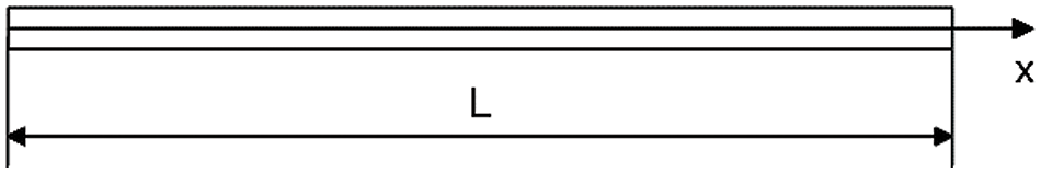
Figure 1: An axial force bar

The elastic modulus is E = 1. The essential boundary condition is given as u0 (x = 0) = 0.5. The continuously distributed load is q(x)=q1+(q2−q1)x/L, where q1 = −3 and q2 = 5. The end of the bar (x = L) is subjected to a concentrated force P = −1. The analytical solution to the problem is given as

u=(q1−q2)x36EAL−q1x22EA+(3L2(q1+q2)+6LP)x6EAL+u0.(38)

18 points are equally distributed within [0, L] for evaluation, and displacement and stress are calculated using a 3-degree PFEM1 (MM = 4) element. Relative errors (%) with the corresponding exact solution are shown in Fig. 2. In Fig. 2, the PFEM1 (p = 3, MM = 4) element achieves high-precision displacement and stress solutions, which indicates the effectiveness and accuracy of the method. From Fig. 2b, it can also be observed that the numerical error is relatively large near the free end. This may be because the node is at the free end, and the element only has C0 continuity at that point, resulting in a higher stress error. However, the error results show that the impact is relatively small.

Figure 2: Relative errors (%) in PFEM1 (p = 3, MM = 4): (a) Displacement u; (b) Stress σ

5.2 An Axial Force Bar Subjected to a Locally Distributed Load

Consider an axial force bar with a length of L = 1 and a cross-sectional area of A = 1. The geometric model is the same as Fig. 1. The elastic modulus is E = 1. The essential boundary conditions are given as u (x = 0) = 0 and u (x = L) = 1. Within the range of [0.48, 0.52], the bar bears a locally distributed load, expressed as

q(x)=2α2−4(α(x−0.5))2e−(α(x−0.5))2   x∈[0.42,0.58],(39)

where α=50. The analytical solution for displacement is given as

u=x+e−(α(x−0.5))2   x∈[0, L],(40)

5.2.1 Uniform Mesh

The mesh and element nodes are shown in Fig. 3, where the black box “□” indicates the mesh boundary, and the red “×” represents element nodes.

Figure 3: Uniform mesh and element nodes

The stress results are obtained using 3-degree four nodes FEM and PFEM1, respectively. The solution domain is divided into 200 elements (601 DOFs), and errors of the numerical solution relative to the exact solution are shown in Fig. 4a. Subsequently, the 5-degree 6-nodes FEM and PFEM1 are used, with 80 elements (401 DOFs), and relative errors are shown in Fig. 4b. In Fig. 4, the results of FEM and PFEM1 show consistency when using the same degree and number of element nodes. Furthermore, a 5-degree element can achieve lower errors with fewer DOFs compared to a 3-degree element. When p = 5, the number of element nodes in PFEM1 is set to 11, with 20 PFEM1 elements (201 DOFs), and the results are compared with FEM in Fig. 4b and shown in Fig. 5. In Fig. 5, PFEM1 (MM = 11) achieves lower stress errors with fewer DOFs compared to FEM (MM = 6).

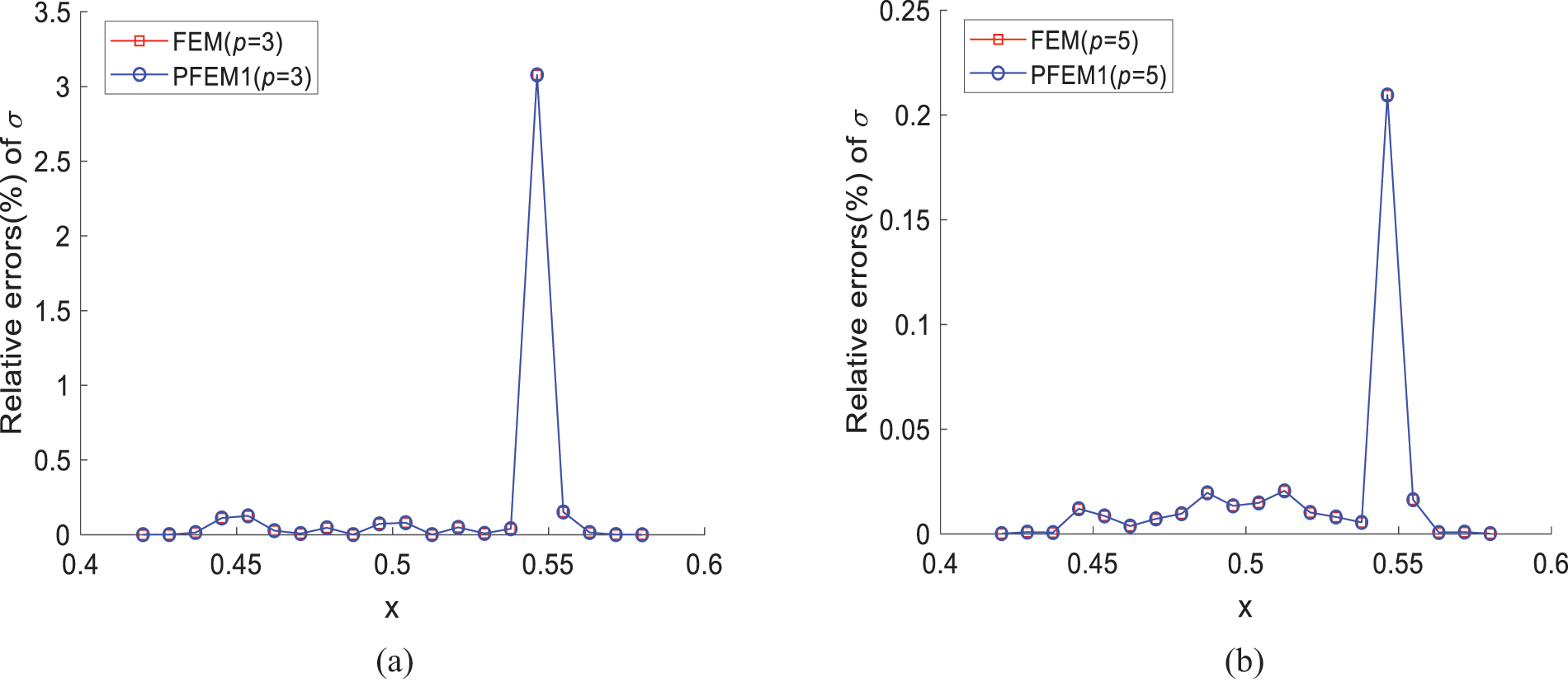
Figure 4: Relative errors of stress σ calculated by FEM and PFEM1: (a) p = 3, MM = 4; (b) p = 5, MM = 6

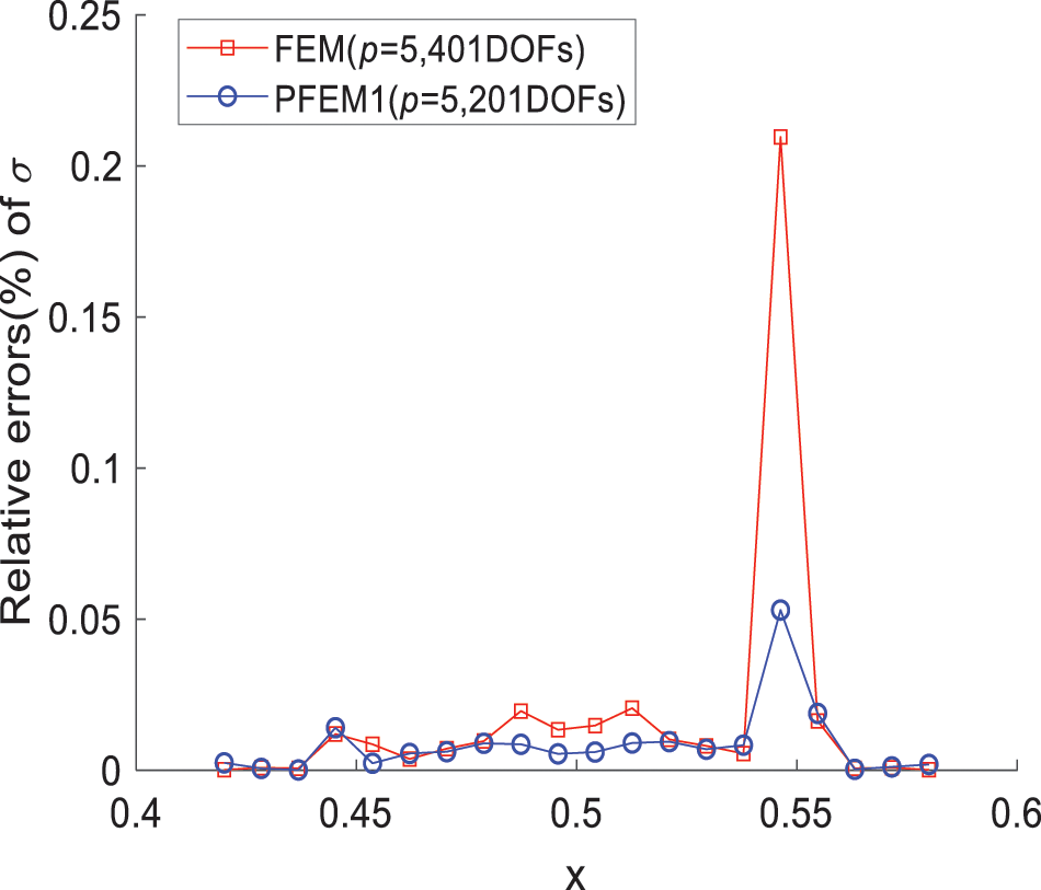
Figure 5: Relative stress errors calculated by PFEM1 (MM = 11) and FEM (MM = 6) when p = 5

Figs. 4 and 5 suggest that the proposed method can improve accuracy by increasing the degree and the number of element nodes. To this end, the improvement of computational accuracy is explored by varying the number of nodes in PFEM1 and the degree of the basis function. Firstly, with p = 5, relative stress errors obtained by PFEM1 elements with different element node numbers are shown in Fig. 6. In Fig. 6a, increasing the number of element nodes can reduce solution errors in the field mutation region. However, in Fig. 6b, as the number of nodes increases to 29 and 31, errors significantly increase. Additionally, with 71 element nodes, the coefficient matrix is prone to singularity as the number of element nodes continues to increase. The possible reason is that the distance between element nodes is too small, leading to large errors and potential matrix singularity. The number of element nodes is set to 16 and 21, respectively, and relative stress errors of PFEM1 with different degrees are shown in Fig. 7.

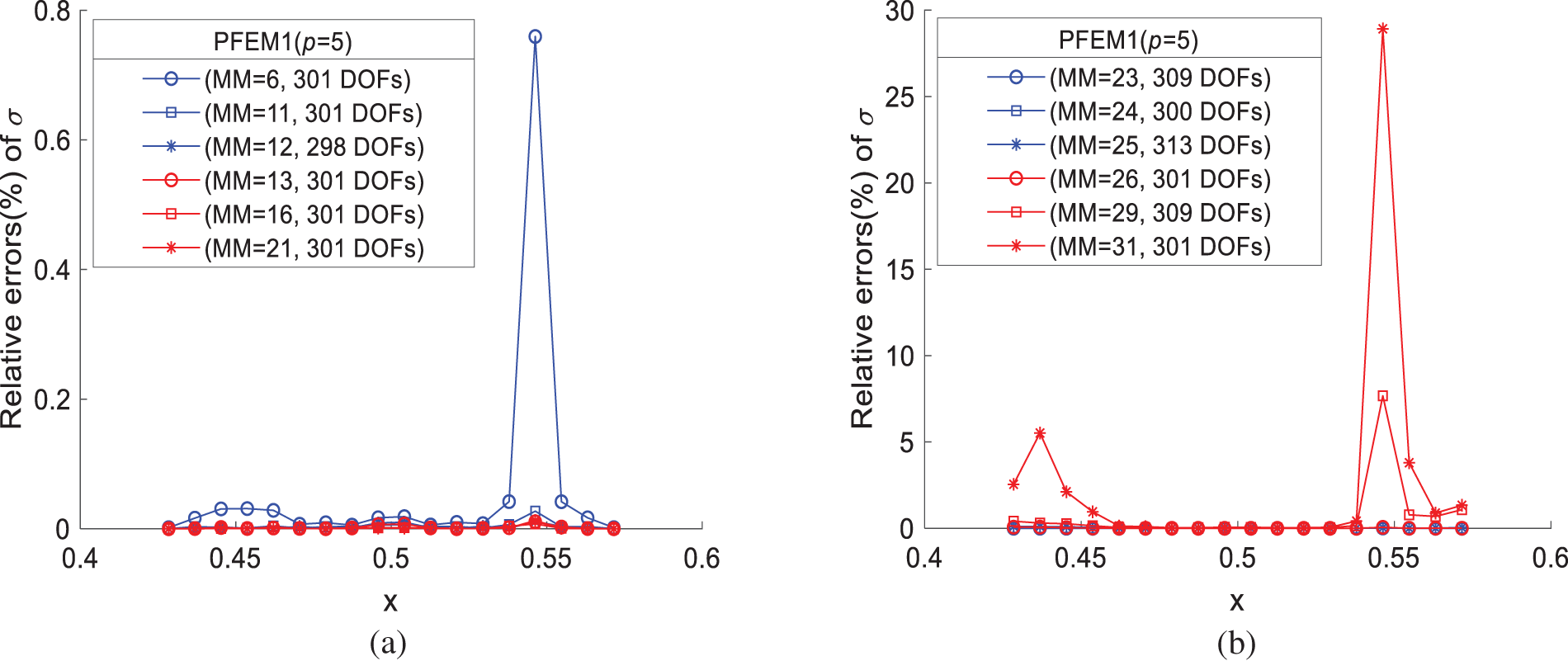
Figure 6: Relative errors of stress obtained in PFEM1 with different node numbers when p = 5: (a) MM = 6, 11–13, 16, 21; (b) MM = 23–26, 29, 31

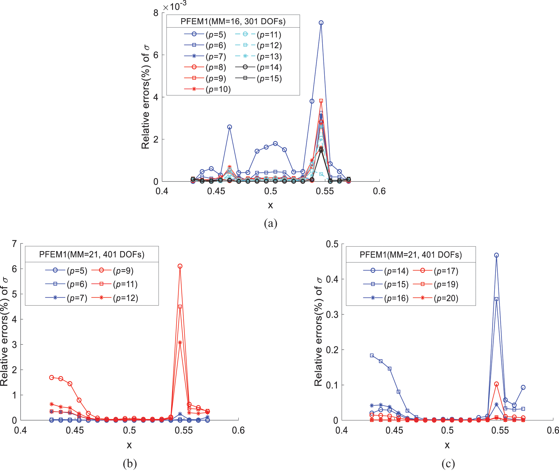
Figure 7: Relative errors of PFEM1 at different degrees when MM = 16 and 21, respectively: (a) p = 5–15, MM = 16; (b) p = 5–7, 9, 11, 12, MM = 21; (c) p = 14–17, 19, 20, MM = 21

Fig. 7a displays results when MM = 16. Fig. 7b,c shows results when MM = 21. In Fig. 7a, when MM = 16, the relative errors decrease as the degree increases. However, when MM = 21, errors with p = 9, 11, 12 are larger, while those with p = 5 are lower. It is evident that MM = 21 is not suitable for elements with p = 9, 11, 12. Overall, the PFEM1 element with MM = 16 yields better results compared to MM = 21. As shown in Fig. 7c, higher-degree basis functions can reduce errors. Reference [20] indicates that the approximation of uniform B-splines is affected by the knot vector. Changes in the number of nodes and the degree of B-splines can alter the knot vector, thereby impacting the approximation quality.

5.2.2 Local Mesh

Firstly, h-refinement is employed and mesh points at x = 0.42, 0.5, 0.58 are inserted into the region with sharp changes in the physical field. The mesh and element nodes are illustrated in Fig. 8. Subsequently, h-refinement is conducted to achieve a relatively dense mesh and nodes in the region, aiming to reduce computational errors. When DOFs are 81, relative errors for FEM (p = 5, MM = 6) and PFEM1 (p = 5, MM = 11) are shown in Fig. 9. In Fig. 9, when p = 5, PFEM1 (MM = 11) can achieve higher precision compared to FEM. Comparatively, local mesh yields high-precision computational results with fewer DOFs than uniform mesh.

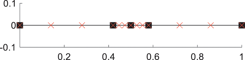
Figure 8: Local mesh and element nodes

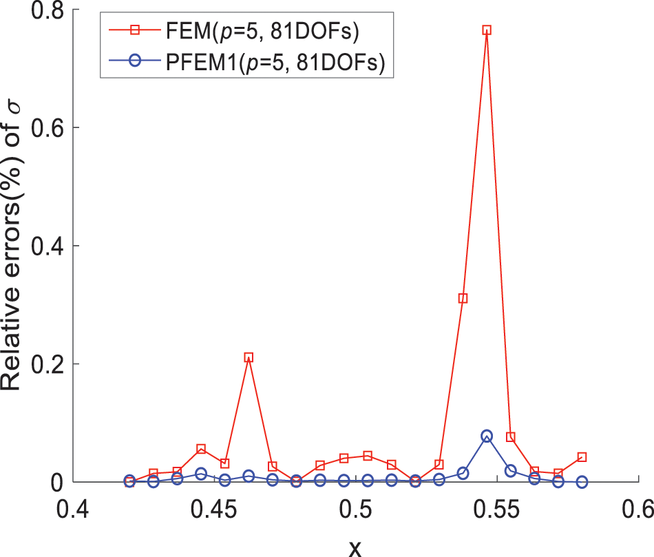
Figure 9: Relative errors calculated by FEM (p = 5, MM = 6) and PFEM1 (p = 5, MM = 11)

Table 1 shows the overall running time of the two elements in Fig. 9 under different DOFs, with t0 and t1 representing the time of PFEM1 and FEM, respectively. In Table 1, when there are a small number of DOFs, the computational efficiency of the PFEM1 (p = 5, MM = 11) element is higher than FEM (p = 5, MM = 6), while as DOFs increase, the computational efficiency between the two is similar.

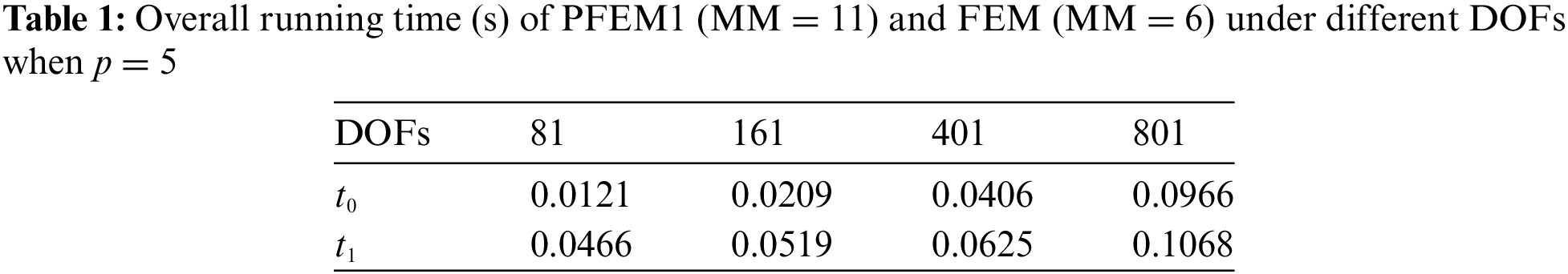
In addition, the overall error formulas are used to compare PFEM1 (MM = 11) and FEM (MM = 6) when p = 5. The L2, H1, and energy norms are expressed as ∫Γ(uh−ue)2dΓ, ∫Γ(u,xh−u,xe)2dΓ and 0.5∫Γ(σh−σe)2dΓ, respectively. The superscripts h and e refer to the numerical and exact solutions, respectively. Fig. 10a–c shows the error results of PFEM1 and FEM, with the x- and y-coordinate represented as base-10 logarithms.

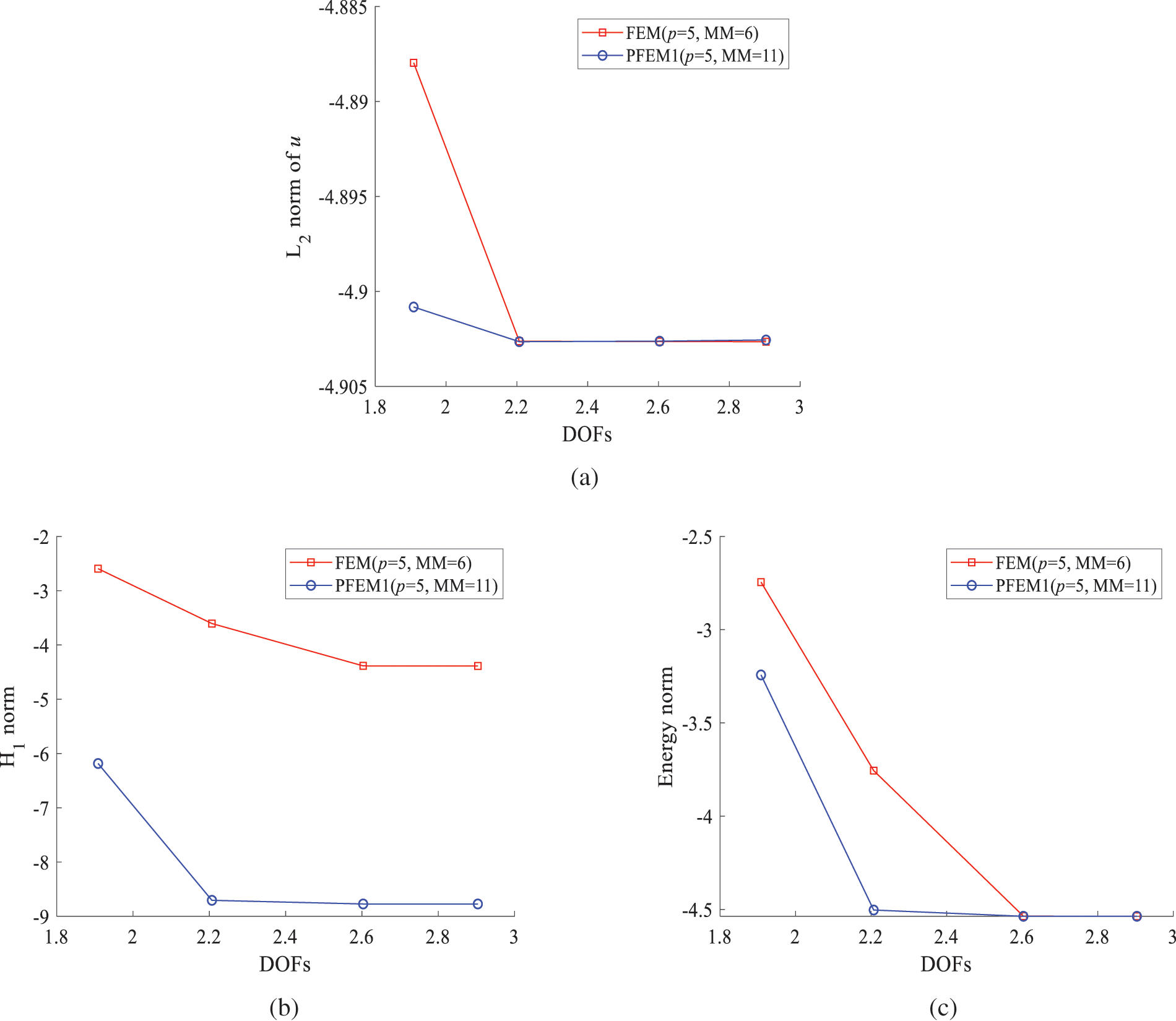
Figure 10: Norm errors of PFEM1 (MM = 11) and FEM (MM = 6) when p = 5: (a) L2 norm; (b) H1 norm; (c) Energy norm

Firstly, it is evident from the three figures that PFEM1 has lower errors with fewer degrees of freedom. Regarding convergence, in Fig. 10a, PFEM1 shows a relatively lower convergence rate compared to FEM when there are fewer degrees of freedom. However, in Fig. 10b,c, PFEM1 exhibits a relatively higher convergence rate. As the degrees of freedom increase, the convergence rates for both types of elements decrease rapidly and approach 0. This may be due to a local field mutation that makes it challenging for polynomial-based basis functions to approximate the solution accurately, thereby limiting the convergence rate. From Figs. 9 and 10, PFEM1 captures sudden physical fields more accurately than FEM and has higher computational accuracy in overall error analysis.

5.3 An Equal Cross-Section Cantilever Beam

A cantilever beam in Fig. 11 is analyzed, with a length of L = 8 and an equal cross-section.

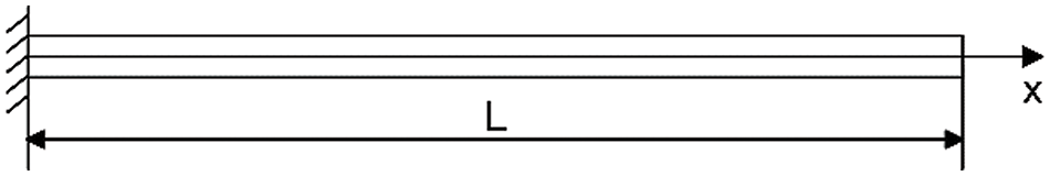
Figure 11: An equal cross-section cantilever beam

The moment of inertia and elastic modulus are I = bh3/12 and E = 2.1e11, respectively. The load conditions are as follows: (1) The entire beam is subjected to a uniformly distributed load q = −1; (2) The free end is subjected to a concentrated force P = −1e5; (3) The free end is subjected to a concentrated bending moment M = −1e7. The corresponding analytical solutions for the boundary conditions (1)–(3) are given as

w=−q24EI(x4−4Lx+6L2),(41)

w=−P6EI(3Lx2−x3),(42)

w=−M2EIx2.(43)

A PFEM1 (p = 4, MM = 5) element is used. 20 evaluation points are equally spaced along the beam. The angle of rotation θ and bending moment M are calculated under boundary condition (1), and relative errors between their results and analytical results are depicted in Fig. 12.

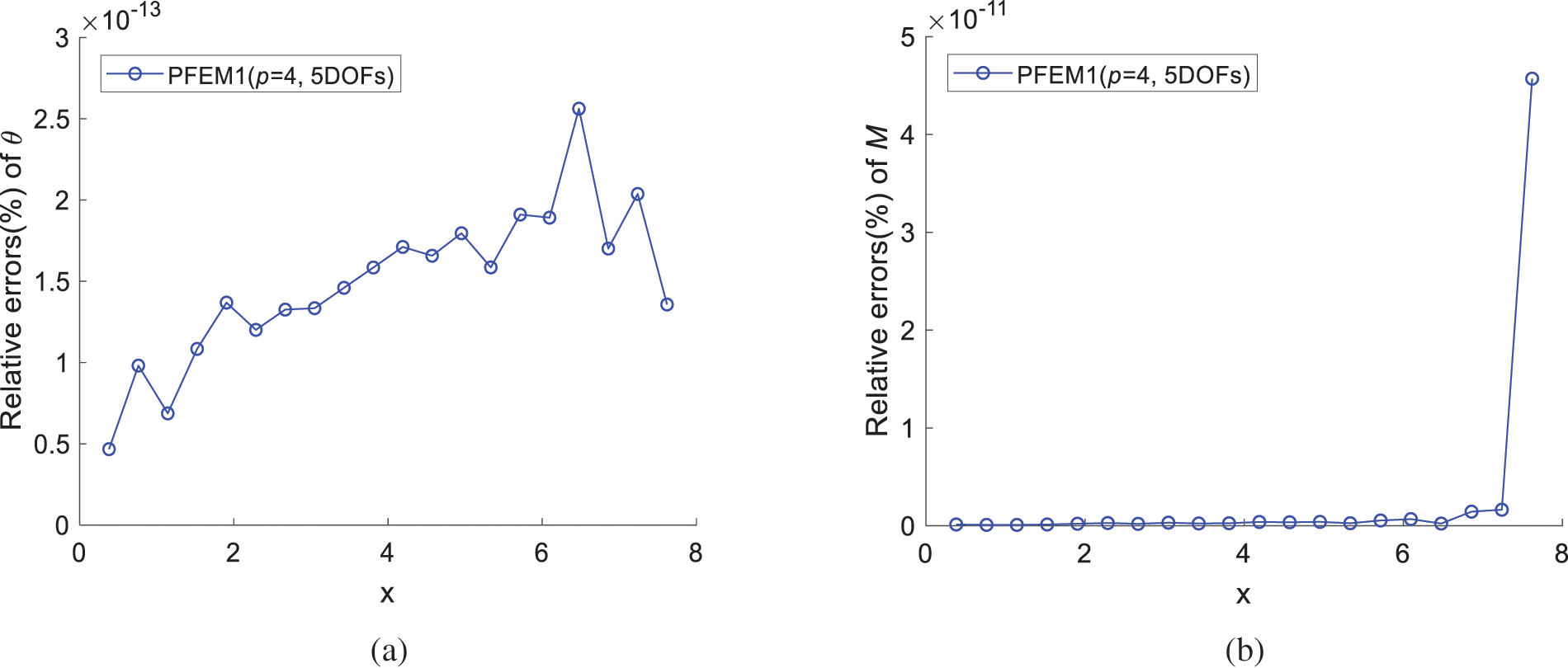
Figure 12: Relative errors obtained using PFEM1 (p = 4, MM = 5) under uniformly distributed load: (a) Angle of rotation θ; (b) Bending moment M

When the beam is subjected to boundary conditions (2) and (3), respectively, relative errors of angle of rotation θ and bending moment M are calculated. Relative errors between their results and analytical results are depicted in Figs. 13, 14.

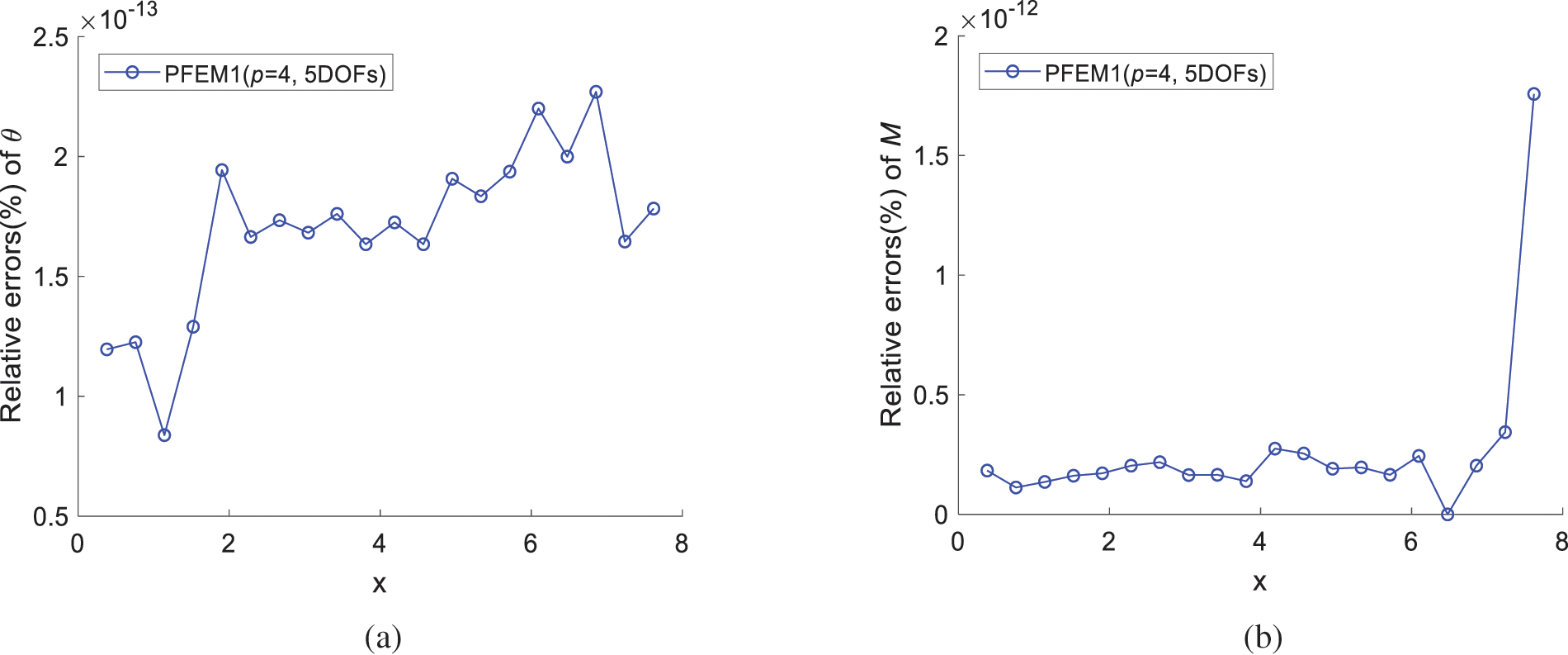
Figure 13: Relative errors obtained using PFEM1 (p = 4, MM = 5) under concentrated force at the free end: (a) Angle of rotation θ; (b) Bending moment M

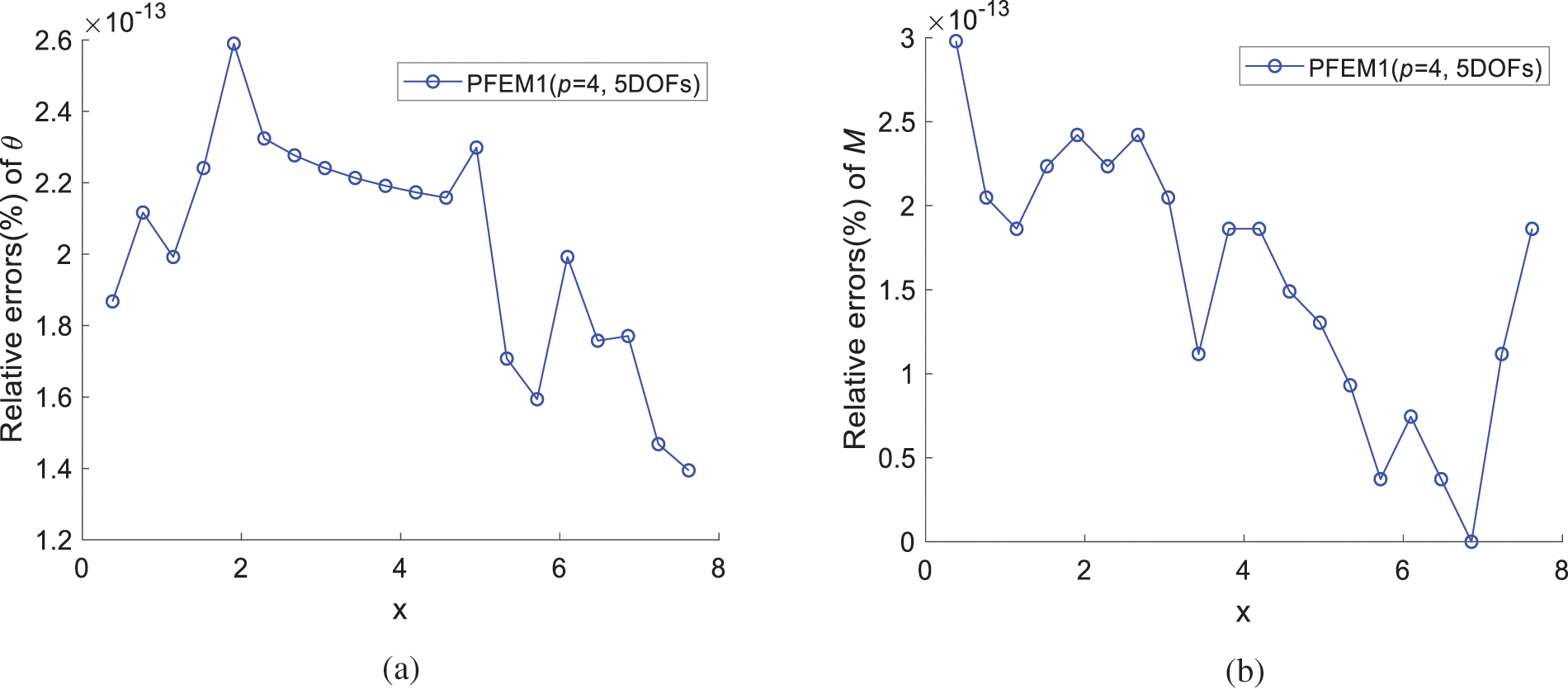
Figure 14: Relative errors obtained using PFEM1 (p = 4, MM = 5) under concentrated bending moment at the free end: (a) Angle of rotation θ; (b) Bending moment M

In Figs. 12–14, the calculated results closely match analytical solutions, demonstrating the high-precision capabilities of the PFEM1 (p = 4, MM = 5) element in solving this problem.

5.4 A Variable Cross-Section Cantilever Beam

A variable cross-section cantilever beam is analyzed in Fig. 15. The length is L = 1, while the width and height of the rectangular section are given as b = 0.1 and h = (1 + 0.9x/L − 1.8 (x/L)2)/10, respectively.

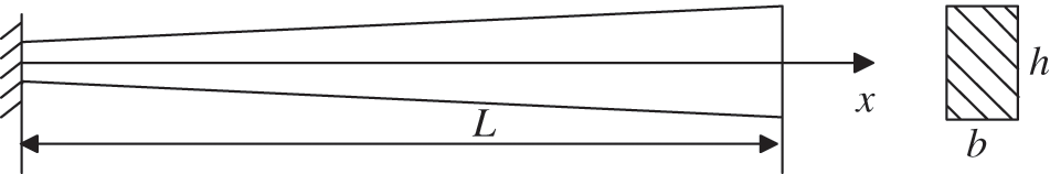
Figure 15: A variable cross-section cantilever beam

The free end is subjected to a concentrated force P = −1. The elastic modulus is E = 1.2e6. The analytical solution for the bending moment is provided in [39]. The numerical solution obtained by FEM and the proposed method is rounded to six decimal places. The equation for calculating the overall relative error (%) is given as

e=1n∑i=1n|uih−uiauia|×100,(44)

where n is the number of evaluation points; uih and uia represent numerical and analytical solutions, respectively. The value of the last evaluation point in the reference solution is 0. To satisfy Eq. (44), the first eight points in [39] are taken as evaluation points. The solution results of the FEM and PFEM1 element with third-degree and two nodes are compared. Uniform h-refinement is used in this example, with the mesh and element nodes shown in Fig. 16.

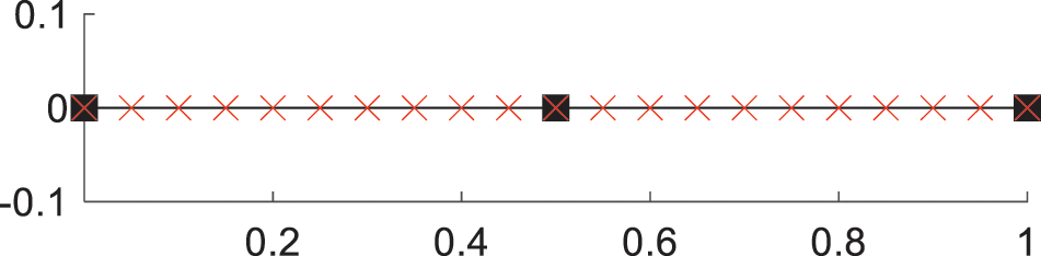
Figure 16: Uniform mesh and element nodes

Fig. 17a displays the error results with increasing DOFs. As can be seen, the results are similar. When MM = 11, the errors obtained by PFEM1 with p = 3, 4, and 5 are compared with those of FEM at the same degree, as depicted in Fig. 17b–d. Fig. 17a,b shows a non-monotonic convergence. The possible reason is that elements based on cubic polynomials are significantly affected by changes in cross-sectional dimensions, leading to unstable numerical results on coarse grids. Increasing the polynomial degree and obtaining a smoother approximation function can help reduce this effect. In Fig. 17b–d, the PFEM1 element can achieve lower errors with fewer DOFs compared to the same degree FEM, indicating good convergence. Among them, the results obtained by the 4- and 5-degree PFEM1 elements are similar, with lower computational errors compared to the 3-degree PFEM1 element. This indicates that the 4-degree PFEM1 element performs better in solving the problem.

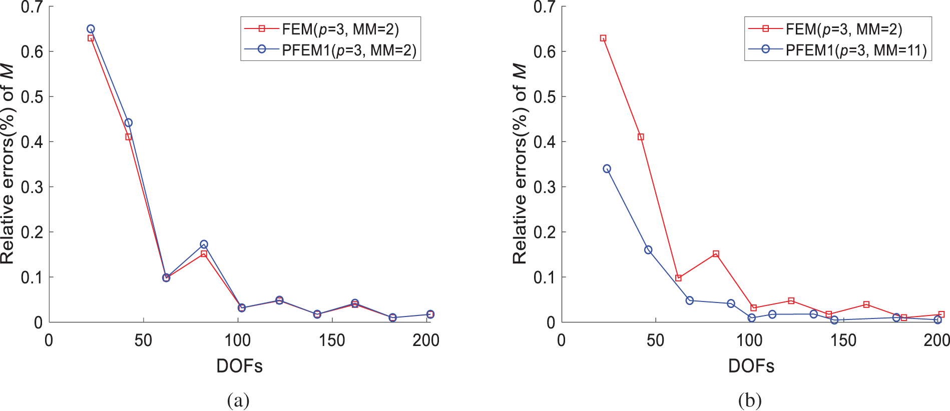
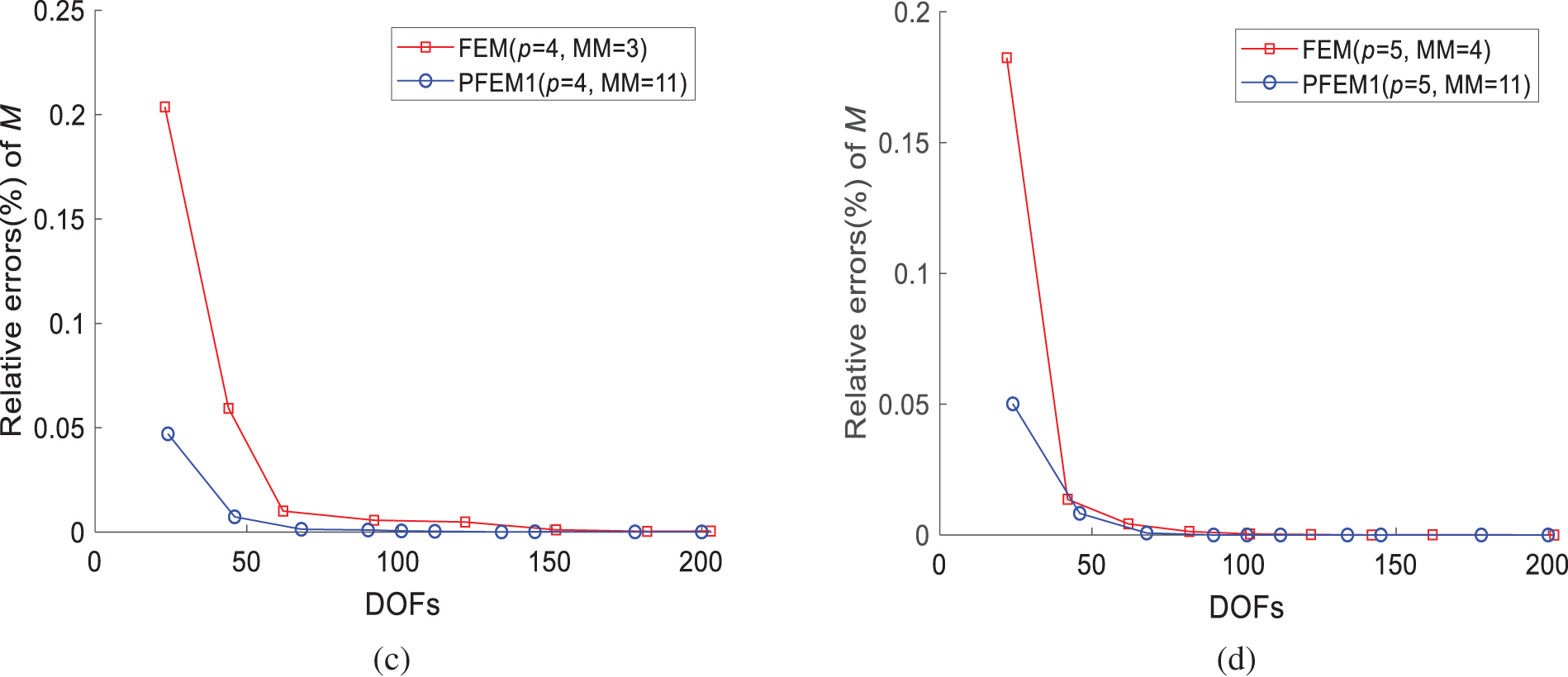
Figure 17: Relative errors of bending moment obtained by FEM and PFEM1: (a) FEM (p = 3, MM = 2) and PFEM1 (p = 3, MM = 2); (b) FEM (p = 3, MM = 2) and PFEM1 (p = 3, MM = 11); (c) FEM (p = 4, MM = 3) and PFEM1 (p = 4, MM = 11); (d) FEM (p = 5, MM = 4) and PFEM1 (p = 5, MM = 11)

Table 2 shows the overall running time of PFEM1 and FEM at different DOFs when p = 3 and MM = 2. In Table 2, t0 and t1 respectively refer to the time of PFEM1 and FEM. It can be seen that under the same DOFs, the proposed method has less running time.

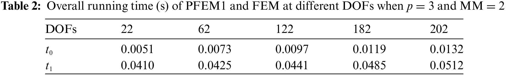
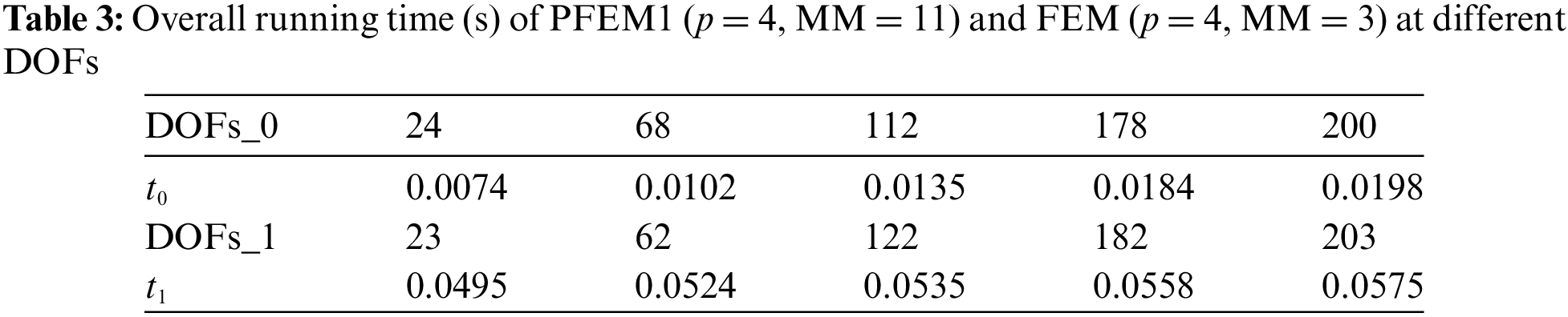
Table 3 shows the overall running time of PFEM1 (p = 4, MM = 11) and FEM (p = 4, MM = 3) at different DOFs, with DOFs_0 and DOFs_1 referring to the DOFs of PFEM1 and FEM, respectively. From Tables 2 and 3, it can be seen that the calculation time of PFEM1 (p = 4, MM = 11) element is relatively less than that of (p = 3, MM = 2) and (p = 4, MM = 3) FEM elements, and is similar to PFEM1 (p = 3, MM = 2) element.

Similarly, a comparison is made between the overall errors of PFEM1 and FEM, with Fig. 18 showing the L2 norm errors of the bending moment M. It can be seen that the proposed method can achieve higher computational accuracy with similar degrees of freedom. In addition, both elements exhibit similar convergence rates as degrees of freedom increase.

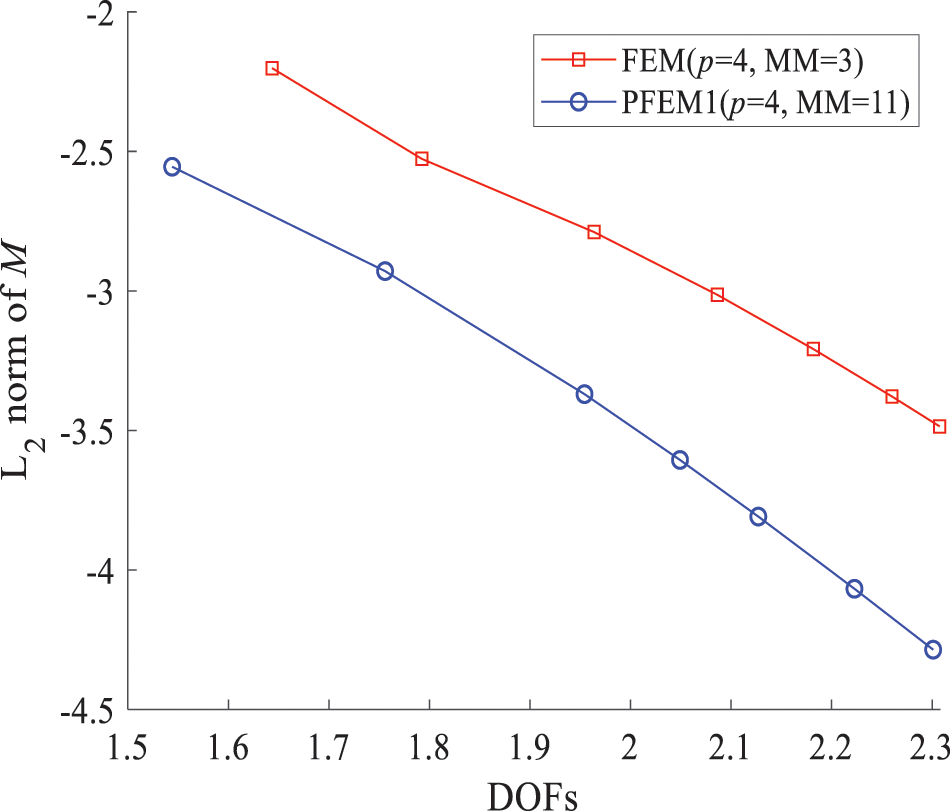
Figure 18: The L2 norm error of the bending moment M for PFEM1 (MM = 11) and FEM (MM = 3) when p = 4

5.5 Lame Problem

In the final example, the plane stress case of Lame’s problem is studied.

A thick hollow cylinder with internal radius a = 8 and external radius b = 10 under constant pressure p = 1 is simulated. Due to the symmetry of the problem, a quarter of the geometric model is established. The geometry and loading conditions are specified in Fig. 19. The elastic modulus and Poisson’s ratio are set to E = 1 and v = 0.3, respectively. For this problem, the analysis solution of the stress field is obtained as [40]

σrr=a2(r2−b2)(b2−a2)r2σrθ=a2p(r2+b2)(b2−a2)r2(45)

where r and θ are the polar coordinates. To evaluate PFEM1, the energy norm is given as 0.5∫Ω(σh−σe)TD−1(σh−σe)dΩ.

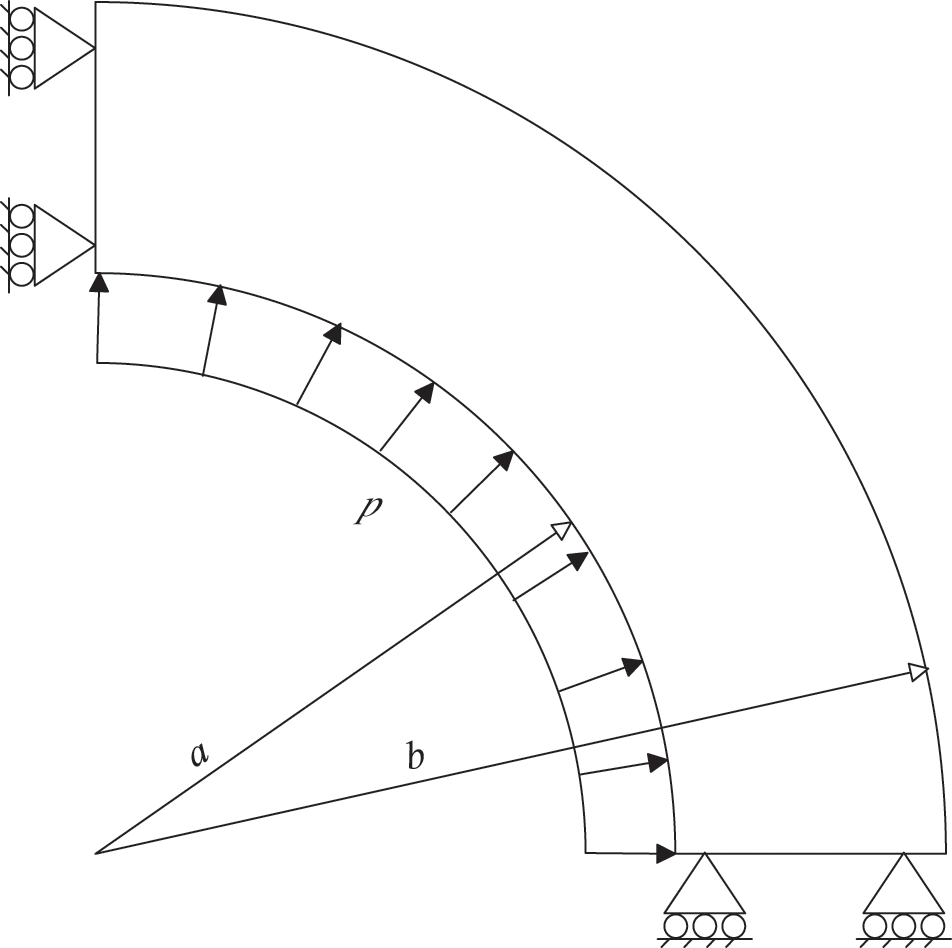
Figure 19: A thick hollow cylinder with lame problem

When the degree is 4 × 4, PFEM1 (MM = 8 × 8) element is constructed and compared with FEM (MM = 5 × 5). Fig. 20 shows the energy norm errors for the two types of elements, abbreviated as PFEM1 (p = 4, MM = 8) and FEM (p = 4, MM = 5).

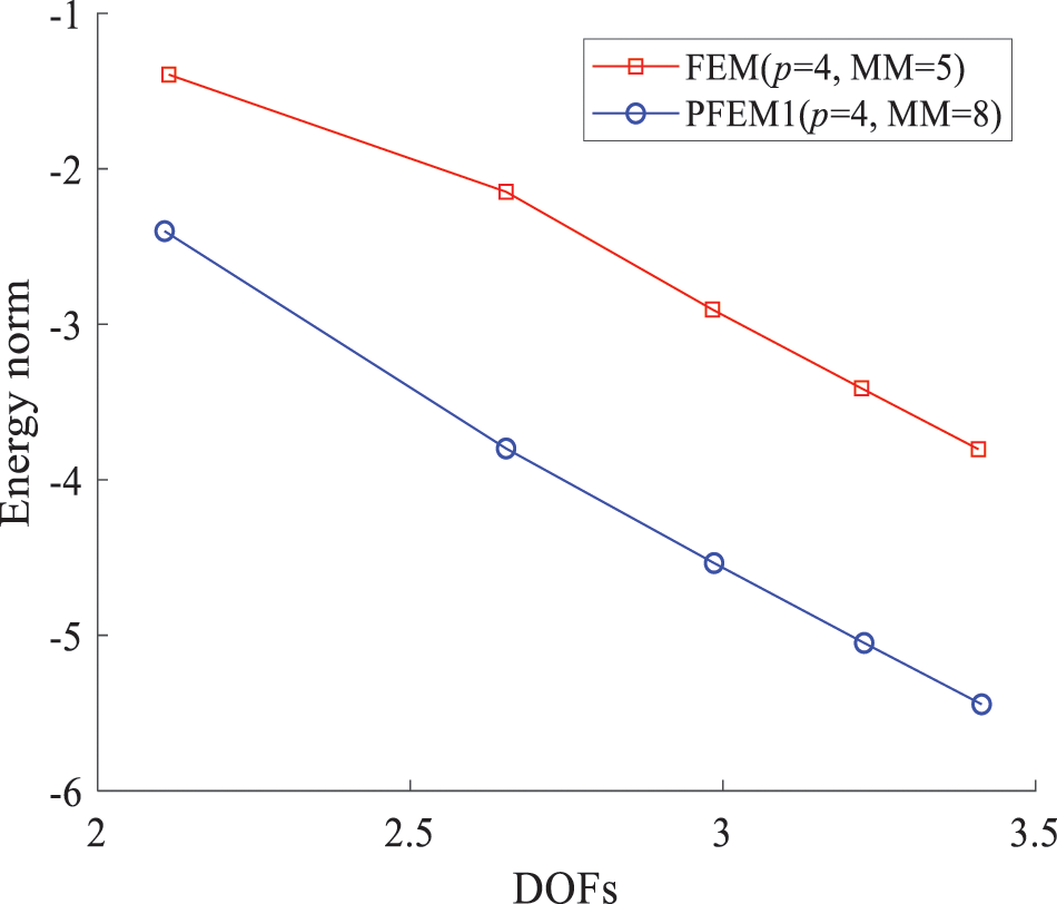
Figure 20: Energy norm errors of PFEM1 (MM = 8) and FEM (MM = 5) when p = 4

From the results, the PFEM1 shows significantly higher computational accuracy with similar degrees of freedom. This is because the geometry of the proposed method is precise, which means there is no geometric discretization error in coarse grids, resulting in lower errors. In addition, the convergence rate is faster with fewer degrees of freedom. However, with grid refinement, the convergence rate remains similar.

6  Conclusions

A method for constructing IGFEM elements is proposed by integrating finite element analysis with isogeometric analysis. The method exhibits the following characteristics: (1) The separation of geometric and physical fields within the element allows for flexible construction. (2) Elements with interpolation properties are constructed, enabling direct application of boundary conditions to nodes. This research presents a new approach for high-performance elements and guides further exploring problems with complex geometric shapes and boundary conditions.

In Examples 1 and 3, the 3-degree C0 type element and 4-degree C1 type element constructed by the proposed method can obtain high-precision solutions; In Example 2, the influence of the number of element nodes and the degree of the basis function on the calculation results of the proposed method is tested. Increasing the number of element nodes or the degree of the basis function can reduce computational errors and improve the convergence rate. However, it should be noted that a small spacing between nodes in an element may also cause significant errors, which can be reduced by increasing the degree of the basis function closer to the number of element nodes; Local mesh refinement can significantly reduce computational errors in areas with significant changes in the physical field, enabling the proposed method to achieve high-precision results with fewer DOFs compared to uniform mesh. In Examples 2 and 4, under the same degree and element node numbers, the proposed method yields similar results as traditional FEM. Additionally, the high-degree and multi-nodes elements constructed by the proposed method have higher computational efficiency under a small number of DOFs, and as the number of DOFs increases to a certain extent, it is similar to FEM. Finally, a curved geometry model with an elasticity problem is tested. As expected, the proposed method can achieve higher computational accuracy under similar degrees of freedom because the method has no geometric errors. In addition, overall error analysis shows that the proposed method offers significantly higher accuracy on coarse grids, while, as the grid is refined, it exhibits the same convergence rate as the finite element method.

Overall, compared to FEM, the proposed method offers a more flexible way of constructing elements, allowing for adjustments in degree and the number of nodes according to the needs of the problem. This improvement enhances computational accuracy and convergence speed. In problems with sharp changes in physical fields and structural size changes, the high-degree, multi-node elements constructed by the proposed method can achieve lower errors with fewer DOFs, leading to more efficient calculations. However, the proposed method has the following limitations: (1) It is difficult to construct high-order continuous elements due to the use of the element interpolation method; (2) For singularity problems (such as local stress concentration and mutations in boundary conditions), the basis functions used are still affected by numerical oscillations, and a more suitable approximation function needs to be constructed. Further in-depth work is required to improve the performance of the method. Furthermore, ongoing efforts are being made to extend the application of this method to two-and three-dimensional structural analysis.

Acknowledgement: None.

Funding Statement: This research was funded by the Zhejiang Province Science and Technology Plan Project under grant number 2023C01069, the Hebei Provincial Program on Key Basic Research Project under grant number 23311808D and the Wenzhou Major Science and Technology Innovation Project of China under grant number ZG2022004.

Author Contributions: The authors confirm contribution to the paper as follows: conceptualization: Pan Su and Jiawei Xiang; methodology, visualization: Pan Su; software: Pan Su and Jiaxing Chen; validation: Pan Su; formal analysis: Pan Su and Jiaxing Chen; investigation, resources: Pan Su and Ronggang Yang; data curation: Pan Su, Ronggang Yang; writing—original draft preparation: Pan Su; writing—review and editing: Jiawei Xiang; supervision: Jiawei Xiang; funding acquisition: Ronggang Yang. All authors reviewed the results and approved the final version of the manuscript.

Availability of Data and Materials: Data sharing is not applicable to this article as no datasets were generated or analyzed during the current study.

Ethics Approval: Not applicable.

Conflicts of Interest: The authors declare that they have no conflicts of interest to report regarding the present study.

References

1. Cen S, Shang Y, Zhou P, Zhou M, Bao Y, Huang J, et al. Advances in shape-free finite element methods: a review. Eng Mech. 2017;34(3):1–14 (In Chinese). doi:10.6052/j.issn.1000-4750.2016.10.0763. [Google Scholar] [CrossRef]

2. Sussman T, Bathe KJ. Spurious modes in geometrically nonlinear small displacement finite elements with incompatible modes. Comput Struct. 2014;140:14–22. doi:10.1016/j.compstruc.2014.04.004. [Google Scholar] [CrossRef]

3. Fries TP, Belytschko T. The extended/generalized finite element method: an overview of the method and its applications. Int J Numer Methods Eng. 2010;84(3):253–304. doi:10.1002/nme.2914. [Google Scholar] [CrossRef]

4. Xiang JW, Chen XF, He ZJ. A new wavelet-based thin plate element using B-spline wavelet on the interval. Comput Mech. 2008;41(2):243–55. doi:10.1007/s00466-007-0182-x. [Google Scholar] [CrossRef]

5. Xiang JW, Chen XF, Yang LF, He ZJ. A class of wavelet-based flat shell elements using B-spline wavelet on the interval and its applications. Comput Model Eng Sci. 2008;23(1):1–12. doi:10.3970/cmes.2008.023.001. [Google Scholar] [CrossRef]

6. Engel G, Garikipati K, Hughes TJR, Larson MG, Mazzei L, Taylor RL. Continuous/discontinuous finite element approximations of fourth-order elliptic problems in structural and continuum mechanics with applications to thin beams and plates, and strain gradient elasticity. Comput Methods Appl Mech Eng. 2002;191(34):3669–750. doi:10.1016/S0045-7825(02)00286-4. [Google Scholar] [CrossRef]

7. Romero I. The interpolation of rotations and its application to finite element models of geometrically exact rods. Comput Mech. 2004;34:121–33. doi:10.1007/s00466-004-0559-z. [Google Scholar] [CrossRef]

8. Taylor RL, Filippou FC, Saritas A. A mixed finite element method for beam and frame problems. Comput Mech. 2003;31:192–203. doi:10.1007/s00466-003-0410-y. [Google Scholar] [CrossRef]

9. Santos HAFA. Complementary-energy methods for geometrically non-linear structural models: an overview and recent developments in the analysis of frames. Arch Comput Methods Eng. 2011;18:405–40. doi:10.1007/s11831-011-9065-6. [Google Scholar] [CrossRef]

10. Santos HAFA. Variationally consistent force-based finite element method for the geometrically non-linear analysis of Euler-Bernoulli framed structures. Finite Elem Anal Des. 2012;53:24–36. doi:10.1016/j.finel.2012.01.001. [Google Scholar] [CrossRef]

11. Mohri F, Eddinari A, Damil N, Ferry MP. A beam finite element for non-linear analyses of thin-walled elements. Thin-Walled Struct. 2008;46(7–9):981–90. doi:10.1016/j.tws.2008.01.028. [Google Scholar] [CrossRef]

12. Xiang JW, Chen DD, Chen XF, He ZJ. A novel wavelet-based finite element method for the analysis of rotor-bearing systems. Finite Elem Anal Des. 2009;45:908–16. doi:10.1016/j.finel.2009.09.001. [Google Scholar] [CrossRef]

13. Zhang W, Zhong Z, Peng C, Yuan W, Wu W. GPU-accelerated smoothed particle finite element method for large deformation analysis in geomechanics. Comput Geotech. 2021;129:103856. doi:10.1016/j.compgeo.2020.103856. [Google Scholar] [CrossRef]

14. Camier JS, Dobrev V, Knupp P, Kolev T, Mittal K, Rieben R, et al. Accelerating high-order mesh optimization using finite element partial assembly on GPUs. J Comput Phys. 2023;474:111808. doi:10.48550/arXiv.2205.12721. [Google Scholar] [CrossRef]

15. Lu Y, Li H, Saha S, Mojumder S, Amin AA, Suarez D, et al. Reduced order machine learning finite element methods: concept, implementation, and future applications. Comput Model Eng Sci. 2021;129(3):1351–71. doi:10.32604/cmes.2021.017719. [Google Scholar] [CrossRef]

16. Hughes TJR, Cottrell JA, Bazilevs Y. Isogeometric analysis: CAD, finite elements, NURBS, exact geometry and mesh refinement. Comput Methods Appl Mech Eng. 2005;194(39–41):4135–95. doi:10.1016/j.cma.2004.10.008. [Google Scholar] [CrossRef]

17. Rauen M, Machado RD, Arndt M. Isogeometric analysis of free vibration of framed structures: comparative problems. Eng Comput. 2017;34(2):377–402. doi:10.1108/EC-08-2015-0227. [Google Scholar] [CrossRef]

18. Praciano JSC, Barros PSB, Barroso ES, Junior EP, Holanda ÁS, Junior JBMS. An isogeometric formulation for stability analysis of laminated plates and shallow shells. Thin-Walled Struct. 2019;143:106224. doi:10.1016/j.tws.2019.106224. [Google Scholar] [CrossRef]

19. Nguyen VP, Anitescu C, Bordas SPA, Rabczu T. Isogeometric analysis: an overview and computer implementation aspects. Math Comput Simul. 2015;117:89–116. doi:10.1016/j.matcom.2015.05.008. [Google Scholar] [CrossRef]

20. Piegl L, Tiller W. The NURBS book. Berlin, Germany: Springer-Verlag; 1997. [Google Scholar]

21. Beer G, Marussig B, Duenser C. The isogeometric boundary element method. Cham, Switzerland: Springer; 2020. [Google Scholar]

22. Luo T, Zhang J, Wu S, Yin SH, He HL, Gong SG. Steady heat transfer analysis for anisotropic structures using the coupled IGA-EFG method. Eng Anal Bound Elem. 2023;154:238–54. doi:10.1016/j.enganabound.2023.05.026. [Google Scholar] [CrossRef]

23. Pan M, Jüttler B, Mantzaflaris A. Efficient matrix assembly in isogeometric analysis with hierarchical B-splines. J Comput Appl Math. 2021;390:113278. doi:10.1016/j.cam.2020.113278. [Google Scholar] [CrossRef]

24. Wen Z, Faruque MS, Li X, Wei X, Casquero H. Isogeometric analysis using G-spline surfaces with arbitrary unstructured quadrilateral layout. Comput Methods Appl Mech Eng. 2023;408:115965. doi:10.1016/j.cma.2023.115965. [Google Scholar] [CrossRef]

25. Li S, Zhao X, Zhou J, Wang X. Quantifying uncertainty in dielectric solids’ mechanical properties using isogeometric analysis and conditional generative adversarial networks. Comput Model Eng Sci. 2024;140(3):2587–611. doi:10.32604/cmes.2024.052203. [Google Scholar] [CrossRef]

26. Yin S, Deng Y, Yu T, Gu S, Zhang G. Isogeometric analysis for non-classical Bernoulli-Euler beam model incorporating microstructure and surface energy effects. Appl Math Model. 2021;89:470–85. doi:10.1016/j.apm.2020.07.015. [Google Scholar] [CrossRef]

27. Fathi F, Borst DR. Geometrically nonlinear extended isogeometric analysis for cohesive fracture with applications to delamination in composites. Finite Elem Anal Des. 2021;191:103527. doi:10.1016/j.finel.2021.103527. [Google Scholar] [CrossRef]

28. Gupta V, Jameel A, Verma SK, Anand S, Anand Y. An insight on NURBS based isogeometric analysis, its current status and involvement in mechanical applications. Arch Comput Methods Eng. 2023;30(2): 1187–230. doi:10.1007/s11831-022-09838-0. [Google Scholar] [CrossRef]

29. Niiranen J, Khakalo S, Balobanov V, Niemi AH. Variational formulation and isogeometric analysis for fourth-order boundary value problems of gradient-elastic bar and plane strain/stress problems. Comput Methods Appl Mech Eng. 2016;308:182–211. doi:10.1016/j.cma.2016.05.008. [Google Scholar] [CrossRef]

30. Khakalo S, Niiranen J. Isogeometric analysis of higher-order gradient elasticity by user elements of a commercial finite element software. Comput-Aided Design. 2017;82:154–69. doi:10.1016/j.cad.2016.08.005. [Google Scholar] [CrossRef]

31. Vo D, Nanakorn P, Bui TQ. A total Lagrangian Timoshenko beam formulation for geometrically nonlinear isogeometric analysis of spatial beam structures. Acta Mech. 2020;231(9):3673–701. doi:10.1007/s00707-020-02723-6. [Google Scholar] [CrossRef]

32. Borković A, Kovačević S, Radenković G, Milovanović S, Guzijan-Dilber M. Rotation-free isogeometric analysis of an arbitrarily curved plane Bernoulli-Euler beam. Comput Methods Appl Mech Eng. 2018;334:238–67. doi:10.1016/j.cma.2018.02.002. [Google Scholar] [CrossRef]

33. Yin SH, Hale JS, Yu T, Bui TQ, Bordas SPA. Isogeometric locking-free plate element: a simple first order shear deformation theory for functionally graded plates. Compos Struct. 2014;118:121–38. doi:10.1016/j.compstruct.2014.07.028. [Google Scholar] [CrossRef]

34. Dvořáková E, Patzák B. Isogeometric Bernoulli beam element with an exact representation of concentrated loadings. Comput Methods Appl Mech Eng. 2020;361:112745. doi:10.1016/j.cma.2019.112745. [Google Scholar] [CrossRef]

35. Apostolatos A, Schmidt R, Wüchner R, Bletzinger KU. A Nitsche-type formulation and comparison of the most common domain decomposition methods in isogeometric analysis. Int J Numer Methods Eng. 2014;94(7):473–504. doi:10.1002/nme.4568. [Google Scholar] [CrossRef]

36. Xiang JW, Chen XF, He YM, He ZJ. The construction of plane elastomechanics and Mindlin plate elements of B-spline wavelet on the interval. Finite Elem Anal Des. 2006;42(14–15):1269–80. doi:10.1016/j.finel.2006.06.00. [Google Scholar] [CrossRef]

37. Xiang JW, Chen XF, He ZJ, Dong HB. The construction of 1D wavelet finite elements for structural analysis. Comput Mech. 2007;40:325–39. doi:10.1007/s00466-006-0102-5. [Google Scholar] [CrossRef]

38. Wang XC. The finite element methods. Beijing, China: Tsing Hua University Press; 2002 (In Chinese). [Google Scholar]

39. Zhang XW, Liu JX, Chen XF, Yang ZB. Multivariable wavelet finite element for plane truss analysis. Comput Model Eng Sci. 2015;109–110(5):405–25. doi:10.3970/cmes.2015.109.405. [Google Scholar] [CrossRef]

40. Timoshenko SP, Goodier JN. Theory of elasticity. 3rd ed. New York, USA: McGraw Hill; 1970. doi:10.3970/cmes.2015.109.405. [Google Scholar] [CrossRef]