Numerical Simulation and Parallel Computing of Acoustic Wave Equation in Isotropic-Heterogeneous Media

1  Introduction

Acoustic wave simulations are foundational in numerous scientific and engineering disciplines, offering insights into wave propagation phenomena crucial for understanding complex systems. Numerical simulations of acoustic wave equations have emerged as indispensable tools, enabling investigations into scenarios that are challenging or impossible to explore through traditional analytical methods or experiments [1].

In this article, we explore the field of numerical modeling aimed at unraveling the intricacies of the two-dimensional acoustic wave equation. However, our study goes beyond conventional simulation to cover a critical real-world characteristic: variable coefficients. Acoustic wave propagation in isotropic-heterogeneous media with spatially varying coefficients is a fundamental problem with diverse applications, including seismology, geophysics, and medical imaging [2]. The investigation of seismic waves involves the analysis of wave propagation in complex media, including interfaces between distinct materials and the interpretation of data recorded in seismographs. Furthermore, the principles developed for this study find application in various fields of knowledge, such as helioseismology [3].

Given its high precision, minimal memory requirements, and rapid computational speed, the finite difference method stands out as a potent tool for simulating acoustic or seismic waves [4–7]. Liao [8] investigated the dispersion, stability, and accuracy of a compact higher-order finite difference scheme for the 3D acoustic wave equation, offering a robust solution to address the complexities of three-dimensional simulations. Building on this work, Liao et al. [9] presented an efficient and precise numerical simulation of acoustic wave propagation in 2D heterogeneous media, underscoring the importance of computational efficiency in practical applications. Li et al. [10] further advanced this field by developing a highly efficient and accurate finite-difference scheme for the 3D acoustic wave equation in heterogeneous media. Their research highlighted the necessity for high-precision solutions in three-dimensional contexts, where media complexity significantly affects wave behavior. Recently, Wu et al. [11] introduced an accurate and efficient local one-dimensional method for the 3D acoustic wave equation, advancing computational methods and providing new insights into the simulation of acoustic waves. However, all proposed numerical solutions are focused mainly on the classical wave equation with a variable coefficient; These equations can generally be used to model wave propagation in anisotropic media. Numerical studies of the wave equation with a variable coefficient, which models the propagation of waves in isotropic media, have been studied relatively little since seismology is a very young branch of science [12]. Numerical studies of the wave equation with a variable coefficient simulating wave propagation in an isotropic medium are well considered in the works of Virieux [13], who showed good results by proposing a staggered-grid scheme, and further, other authors presented their solutions [14–16].

In practice, physical phenomena must be simulated over a large area and over a long time; if the computational algorithm is sequential, this leads to a significant investment of time and energy. Therefore, the most effective way to solve this problem is parallel computing. Modern computers are multi-core and heterogeneous, so computing algorithms must be based on parallel computing to take full advantage of the computer’s capabilities. One of the parallel computing technologies is GPU. Graphics Processing Units (GPUs) represent a notable parallel computing technology. They provide highly parallelized processors with multiple threads and cores, delivering substantial computational power. The appeal of GPUs lies in their cost-effectiveness, high bandwidth for floating-point operations, and efficient memory access. This makes them an increasingly attractive option for high-performance computing. In contrast to conventional cluster systems, GPUs offer a cost-effective alternative with comparable performance and lower power consumption [17]. Researchers across diverse scientific and technological fields have observed significant enhancements in productivity by harnessing the computational capabilities offered by GPUs [18–22].

To solve high-dimensional problems, using an implicit scheme, a block tridiagonal system arises, solved at each time step. A direct solution of such a large-scale block linear system is ineffective, so operator separation methods are used to transform a high-dimensional problem into a sequence of one-dimensional problems. One commonly used method is the ADI (Alternating Direction Implicit) method, which was originally proposed for solving parabolic and elliptic equations by Peaceman et al. [23]. Over the years, many developments have been made in the field of hyperbolic equations [24–26].

Recent advancements in numerical methods and computational capabilities have facilitated more sophisticated simulations of wave behavior in complex media. For instance, Wei et al. [27] examined the numerical simulation of anti-plane wave propagation in heterogeneous media, revealing the intricate interactions between waves and material heterogeneities. Similarly, Wei et al. [28] introduced a 2.5D singular boundary method for acoustic wave propagation, offering a robust framework for simulating wave phenomena with heightened accuracy and efficiency.

The influence of environmental factors on acoustic wave propagation has also received considerable attention. Coyle et al. [29] studied the effects of internal waves on underwater acoustic propagation, underscoring the dynamic nature of underwater acoustic environments and the need for adaptive modeling approaches. Zeng et al. [30] conducted a theoretical and numerical analysis of transient acoustic wave propagation across ice layers in the Arctic Ocean, addressing the unique challenges posed by polar environments.

In the field of anisotropic media, Luis et al. [31] extended Snell’s Law for the propagation of acoustic waves in elliptically anisotropic media, thereby expanding the theoretical framework for wave behavior in complex anisotropic settings. Additionally, Xue et al. [32] explored the propagation mechanisms of leakage acoustic waves in gas-liquid stratified flow, providing essential insights into the acoustic properties of multiphase systems.

In this study, our goal is to perform numerical simulations of acoustic wave propagation in heterogeneous media using a GPU. We aim to identify the potential benefits and effectiveness of this approach. By harnessing the processing power of GPUs and Compute Unified Device Architecture (CUDA) technology, our goal is to make meaningful contributions to the field of numerical simulation of the variable coefficient acoustic wave equation.

2  Problem Statement and Numerical Scheme

We consider the following equation that describes the propagation of acoustic waves in the isotropic-heterogeneous medium:

∂2p∂t2−[∂∂x(q(x,y)∂p∂x)+∂∂y(q(x,y)∂p∂y)]=s(t,x,y),(t,(x,y))∈[0;T]×Ω;(1)

p(0,x,y)=ψ1(x,y),(x,y)∈Ω;(2)

∂p(0,x,y)∂t=ψ2(x,y),(x,y)∈Ω;(3)

p(t,x,y)=φ(t,x,y),t∈[0,T],(x,y)∈∂Ω;(4)

Here, p is pressure, q is a variable coefficient that describes heterogeneous medium, s is the source function, ψi,φ are known functions.

First assume that Ω is a 2D rectangular domain: [x0,x1]×[y0,y1], which is discretized into an Nx×Ny grid with spatial grid sizes hx,hy. Let τ be the time stepsize and pi,jk denote the numerical solution at the grid point (xi,yj) and time level kτ.

The approximate solution is calculated at discrete points of the space-time grid Ωhx,hyτ: Ωh1,h2τ={xi=ih1,i=0,Nx¯;yj=jh2,j=0,Ny¯;tk=kτ,k=0,1,2…M}.

To approximate problems (1)–(4), we use the finite difference method. For simplicity, we put N:=Nx=Ny and denote h:=hx=hy. Let us consider the Crank-Nicholson scheme for the problem (1)–(4). First, we transform the partial differential Eq. (1) into an implicit finite-difference equation.

pi,jk+1−2pi,jk+pi,jk−1τ2−qi,jk2h2((pi+1,jk+1−2pi,jk+1+pi−1,jk+1+pi+1,jk−1−2pi,jk−1+pi−1,jk−1)+(pi,j+1k+1−2pi,jk+1+pi,j−1k+1+pi,j+1k−1−2pi,jk−1+pi,j−1k−1))−(qi+1,jk−qi−1,jk2h)(pi+1,jk−pi−1,jk2h)−(qi,j+1k−qi,j−1k2h)(pi,j+1k−pi,j−1k2h)=si,jk;(5)

for (k,i,j)∈ωh,hτ, where qi,jk:=q(ih,jh), si,jk:=s(kτ,ih,jh) with initial conditions

pi,j0=φi,j,pi,j1−pi,j0=τφi,j;(6)

for (i,j)∈0,N¯×0,N¯, and with boundary conditions

p0,jk=0,pN,jk=0,pi,0k=0,pi,Nk=0;(7)

for (j,k)∈0,N¯×0,M¯ and (i,k)∈0,N¯×0,M¯, respectively. The implicit finite difference scheme (5) has an accuracy order of O(τ2+h2).

Next, implementing the ADI method to the Eq. (5), we split it into two sub-equations. In the ADI method, each numerical step is divided into several sub-steps depending on the spatial dimension of the problem. A system of linear equations is solved implicitly in one direction, while information in the other (or other) directions is processed explicitly. This alternate approach makes the ADI method unconditionally robust, providing second-order accuracy in both time and space. An additional positive property of the ADI method is that at each substage the equations to be solved have a tridiagonal structure, which makes it possible to effectively use the tridiagonal matrix algorithm (TDMA) to solve them.

For problem (5), the ADI method has the form

pi,jk+1/2−2pi,jk+pi,jk−1/2τ2−qi,j4h2(pi+1,jk+1/2−2pi,jk+1/2+pi−1,jk+1/2+pi+1,jk−1/2−2pi,jk−1/2+pi−1,jk−1/2)−(qi+1,j−qi−1,j2h)(pi+1,jk−1/2−pi−1,jk−1/22h)=si,jk−1/2;(8)

and

pi,jk+1−2pi,jk+1/2+pi,jkτ2−qi,j4h2((pi,j+1k+1−2pi,jk+1+pi,j−1k+1)+(pi,j+1k−2pi,jk+pi,j−1k))−(qi,j+1−qi,j−12h)(pi,j+1k−pi,j−1k2h)=si,jk;(9)

2.1 Stability Analysis

In this subsection, we consider the von Neumann stability analysis [33] to analyze the stability of the finite difference schemes 8 and 9. The von Neumann stability analysis method is a common tool for assessing the stability of numerical methods such as finite difference methods or finite element methods in the numerical solution of partial differential equations (PDE). In this problem the coefficient qi,j is not constant, so to implement the von Neumann stability analysis, we use the principle of frozen coefficients [34]. Here we perform stability analysis for Eqs. (8), and (9) is analyzed similarly. To investigate the stability of the scheme, we start with the usual ansatz

pi,jk+1/2=ξk+1/2eIβxiheIβyjh;

where βx and βy are the wave number in x and y, I=−1, h is spatial step size in x and y, i is the spatial index in x, j is the spatial index in y, ξ is the amplification factor.

Replacing the expression above into the Eq. (8) yields:

ξk+1/2eIβxiheIβyjh−2ξkeIβxiheIβyjh+ξk−1/2eIβxiheIβyjh−rqi,j[(ξk+1/2eIβx(i+1)heIβyjh−2ξk+1/2eIβxiheIβyjh+ξk+1/2eIβx(i−1)heIβyjh+ξk−1/2eIβx(i+1)heIβyjh−2ξk−1/2eIβxiheIβyjh+ξk−1/2eIβx(i−1)heIβyjh)]−rqi,ja(ξk−1/2eIβx(i+1)heIβyjh−ξk−1/2eIβx(i−1)heIβyjh)=si,jk−1/2;(10)

where r=τ24h2, qi,ja=qi+1,j−qi−1,j

After dividing by ξkeIβxiheIβyjh and simplifying Eq. (10), we have

ξ1/2−2+ξ−1/2−rqi,j[(ξ1/2eIβxh−2ξ1/2+ξ1/2e−Iβxh+ξ−1/2eIβxh−2ξ−1/2+ξ−1/2e−Iβxh)]+ξ−1/2rqi,ja(eIβxh−e−Iβxh)=0;(11)

Let G=ξ1/2 then we can rewrite it as therefore

G2(1+4rqi,j(sin2βxh2))−2G+1+4rqi,j(sin2βxh2)−rqi,jaIsin(βxh)=0;(12)

Clearly, the maximum value of the sin function is 1, and since r and qi,j are real numbers, the discriminant (D) of a quadratic Eq. (12) is always greater than 0. Therefore, two distinct real solutions exist. For stability, ξ1 and ξ2 must be less than or equal to 1. In general, for the quadratic equation ax2+bx+c=0 to have solutions that are less than or equal to 1, the following inequality must hold: −b±D2a≤1.

If we substitute our values into this inequality, we get 12≥−2rqi,ja±D. After analyzing the discriminant, we consistently find that it remains below 2, and the previously mentioned inequality is consistently met. Consequently, we can assert that |(ξ1,ξ2)2| remains equal to or less than 1, leading us to conclude that the equation scheme exhibits unconditional stability.

Eqs. (8) and (9) are in the form of a tridiagonal matrix and will be solved individually by the Tridiagonal matrix algorithm. In practice, the three most widely used methods are the Thomas method [35], the cyclic reduction (CR) [36] method, and the parallel cyclic reduction (PCR) method [37]. The Thomas method, characterized by a sequential approach, turns out to be ineffective for parallelization on GPUs. In this regard, preference is given to the PCR method, which provides more efficient parallelization and solution of tridiagonal systems of equations. The CR method is an efficient algorithm for solving tridiagonal linear systems of equations that often arise in the process of discretizing partial differential equations. The basic idea of the CR is to successfully reduce the size of a linear system by a factor of two at each step until the system can not be solved directly [37,38].

2.2 Numerical Accuracy Analysis

We assess the numerical solution’s accuracy obtained through the finite-difference method by calculating both the absolute error and the L2 norm error. These errors are defined as follows:

errabs=|p−pnum|(13)

L2=∑i=1n(p−pnum)2ΔxΔy(14)

where p represents the exact value, and pnum is the numerical approximation. We use the unit square (x,y)∈[0,1]×[0,1] as the spatial domain, with 100 elements per side and 100 interior points. The parameters are q(t,x,y)=1, s(t,x,y)=0, with the initial condition p(x,y,0)=sin⁡(2πx)sin⁡(2πy), ∂p(x,y,0)∂t=0, and boundary conditions p(0,y,t)=p(1,y,t)=p(x,0,t)=p(y,1,t)=0. The analytical solution of the Eq. (1) is given by p(x,y,t)=cos⁡(2π2t)sin⁡(2πx)sin⁡(2πy).

Table 1 presents the absolute error and L2 norm error for various time and spatial step sizes.

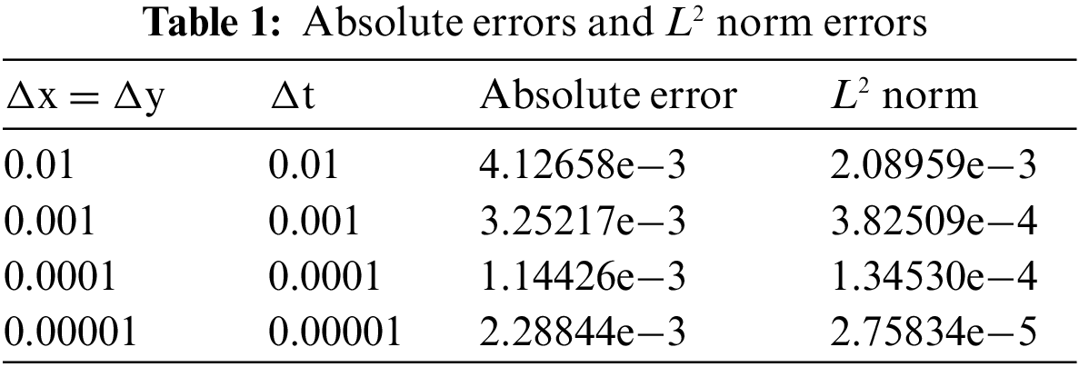
From Table 1, it is evident that the numerical solution closely matches the analytical solution, highlighting their strong agreement. The table displays the absolute error, with the smallest magnitude being 10−3. This demonstrates the method’s high accuracy and its effectiveness in simulating wave equations.

2.3 Numerical Simulations

In this section, we do numerical simulations for the wave propagation in two heterogeneous mediums with the Dirichlet boundary condition in the domain [0,T]×[0,200]×[0,200]. The two heterogeneous mediums are shown in the Fig. 1.

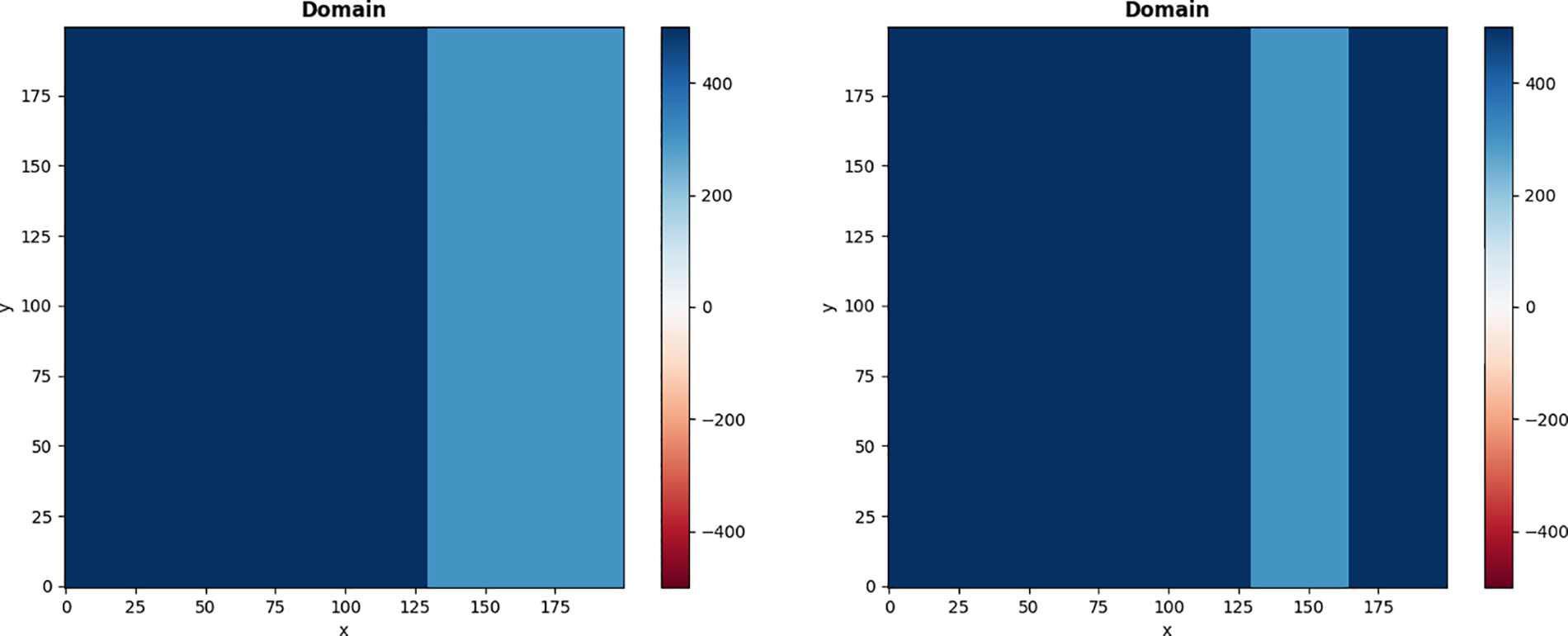
Figure 1: Two heterogeneous mediums: a two-layer medium on the left and a three-layer medium on the right

As a source term function, we use the Ricker’s wavelet function given by

s(x,y,t)=δ(x−x0)δ(y−y0)(1−2π2f02(t−t0)2)e−π2f02(t−t0)2

where δ(x−x0)δ(y−y0) is the Dirac distribution, f0 represents the dominant frequency of the source, which controls the central frequency of the wavelet. The graphical illustration of the source function is shown in the Fig. 2. In the first case, a two-layer medium is considered, characterized by a homogeneous left half with a seismic speed s1=500 m/s and a homogeneous right half with a speed s2=250 m/s. The source is located at point (x0,y0)=(100 m,100 m). In the second case, a three-layer medium is considered with velocities s1=500 m/s in the left layer, s2=250 m/s in the middle layer and s3=500 m/s in the right layer. Computational parameters include spatial step size Δx=Δy=1 m and time step size Δt=0.001 s.

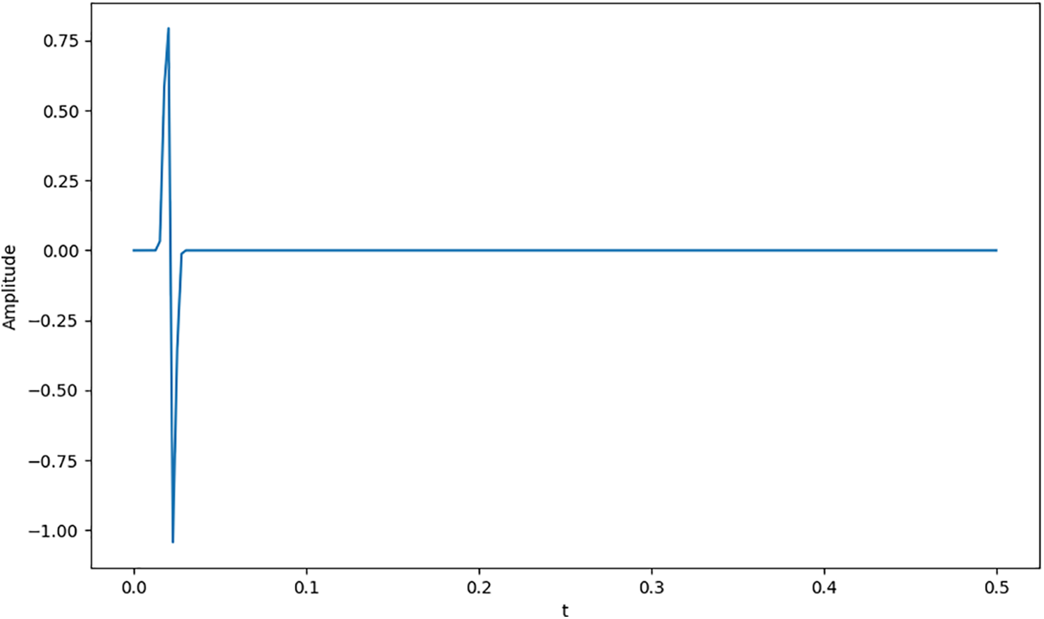
Figure 2: Source waveform

Fig. 3 presents snapshots of wavefields at different times in a two-layer medium. At t=0.05 s, the wavefront forms a precise circle before reaching the interface between the two layers. By t=0.15 s, the wavefront interacts with the interface, resulting in moderate reflection. As both layers are homogeneous, the reflected and refracted wavefronts form perfect circles in the left and right halves of the domain, respectively. At t=0.25 s and t=0.30 s, both the reflected and refracted waves continue to propagate. Due to the higher wave velocity in the left layer compared to the right layer, the wave circle in the left layer is larger. Simultaneously, the amplitude of the reflected wave in the right layer appears relatively weak.

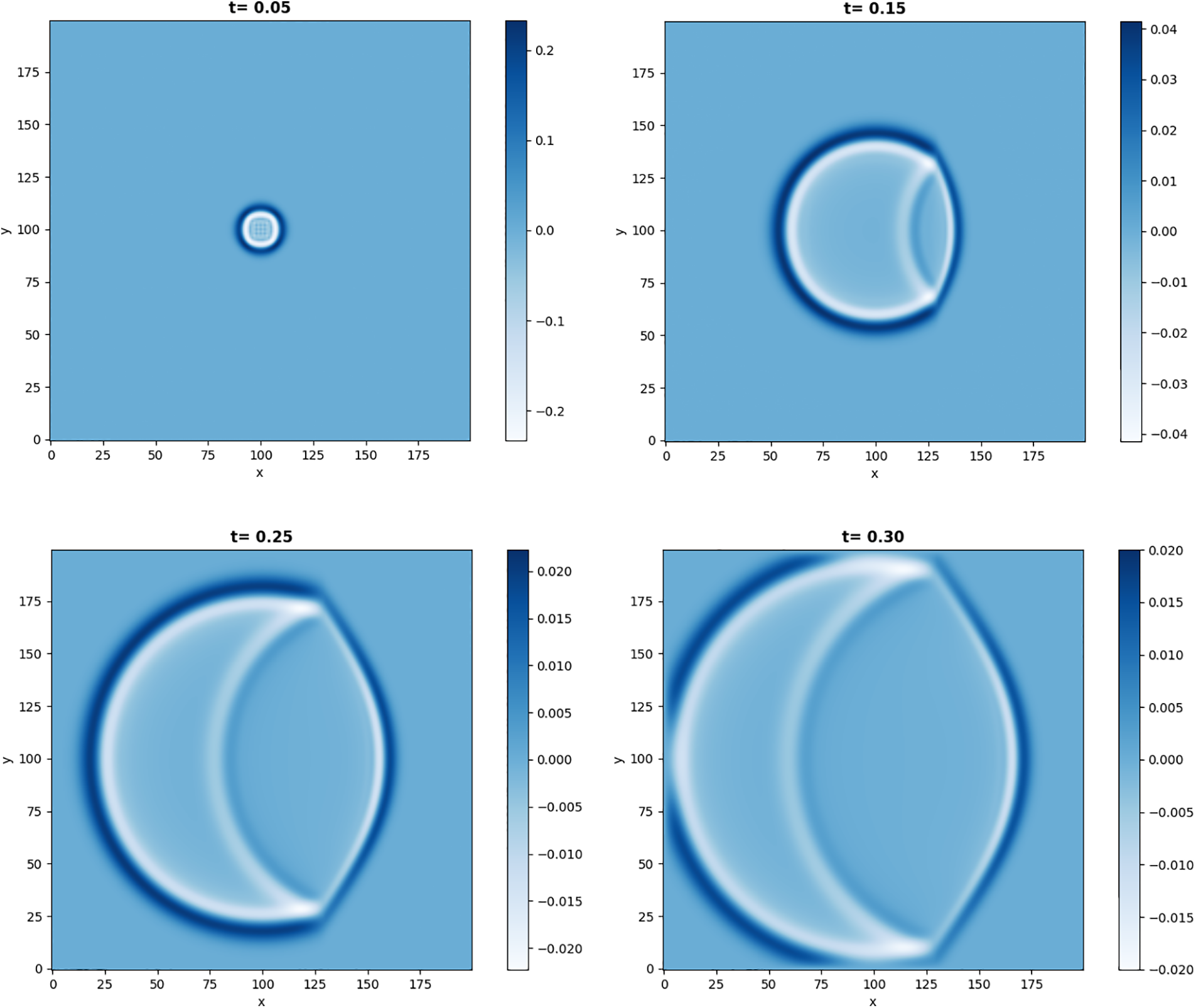
Figure 3: Displacement of wave in the two-layer medium at different times

Fig. 4 shows snapshots of wavefields at different time intervals in a three-layer medium. At t = 0.20 s, the wave predominantly propagates within the middle layer. By t = 0.30 s, the wavefront interacts with both the left and right interfaces, resulting in observable reflection phenomena within the middle layer. As time progresses, both the reflected and refracted waves continue to propagate, forming precise circular wavefronts, as evident at t = 0.32 s.

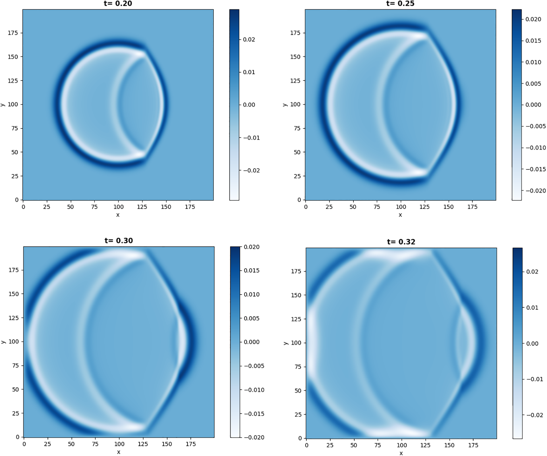
Figure 4: Displacement of wave in the three layers medium at different times

3  GPU Implementation

Parallel processing on GPUs has emerged as a pivotal area in computational science, significantly transforming the landscape of high-performance computing. GPUs, originally designed for rendering graphics in video games, have demonstrated exceptional capabilities in parallel processing due to their massively parallel architecture [39].

One of the key advantages of GPUs is their ability to handle a large number of simple tasks simultaneously. This is achieved through the presence of multiple cores, often numbering in the thousands, allowing GPUs to execute parallel threads efficiently. Unlike traditional Central Processing Units (CPUs), which are optimized for sequential processing, GPUs excel in parallelizing tasks, making them particularly well-suited for applications with a high degree of parallelism.

Scientific simulations, such as those used in physics, chemistry, and fluid dynamics, have witnessed remarkable acceleration through GPU parallel processing. The parallel architecture of GPUs enables researchers to break down complex simulations into smaller, manageable tasks that can be processed simultaneously. This not only significantly reduces the time required for simulations but also opens up the possibility of exploring more intricate and computationally intensive models.

However, to exploit the full potential of GPU parallel processing, special programming techniques are required. CUDA and OpenCL (Open Computing Language) are two widely used frameworks that allow developers to create parallel applications for GPUs.

In this section, we introduce a parallel approach using CUDA technology to numerically solve problem 1 and then analyze its performance. The parallel approach structure is shown in Fig. 5. The kernel function shown in this figure refers to implementing the PCR [37] in CUDA. We will describe the PCR method in the following subsections.

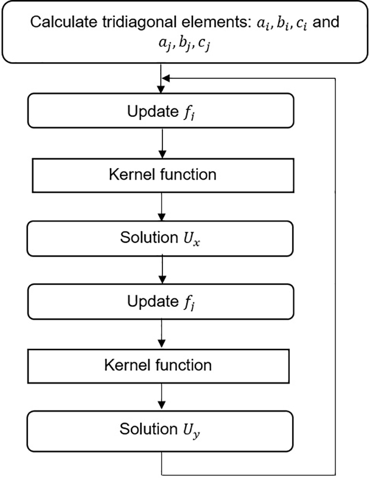
Figure 5: Parallel solver

3.1 CUDA Technology

CUDA is a revolutionary parallel computing technology developed by NVIDIA, designed to harness the immense computational power of GPUs for general-purpose computing tasks. Introduced in 2007, CUDA extends the capabilities of GPUs beyond graphics processing, enabling developers to exploit parallelism for a wide range of applications. At the heart of CUDA is the integration of parallel constructs into the C programming language, allowing developers to write code that takes advantage of the parallel architecture inherent in modern GPUs. The parallel part is called the kernel. A C program using CUDA extensions hands out a large number of copies of the kernel into available multiprocessors to be performed contemporaneously. The CUDA code consists of three computational steps: transferring data to the global GPU memory, running the CUDA kernel, and transferring the results from the GPU to the CPU memory.

The Parallel Cyclic Reduction method is a parallelized version of the Cyclic Reduction algorithm designed to efficiently solve large-scale tridiagonal systems of linear equations on parallel computing architectures. The process of the Parallel Cyclic Reduction method data flow with an 8-equation system is illustrated in Fig. 6. This process involves reducing the 8-equation system to two 4-equation systems in the first step, followed by reducing two 4-equation systems to four systems of 2 equations, and finally solving four systems in the third stage [40]. We have designed a CUDA program based on Parallel Cyclic Reduction.

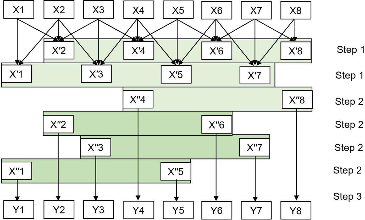
Figure 6: Data flow of PCR

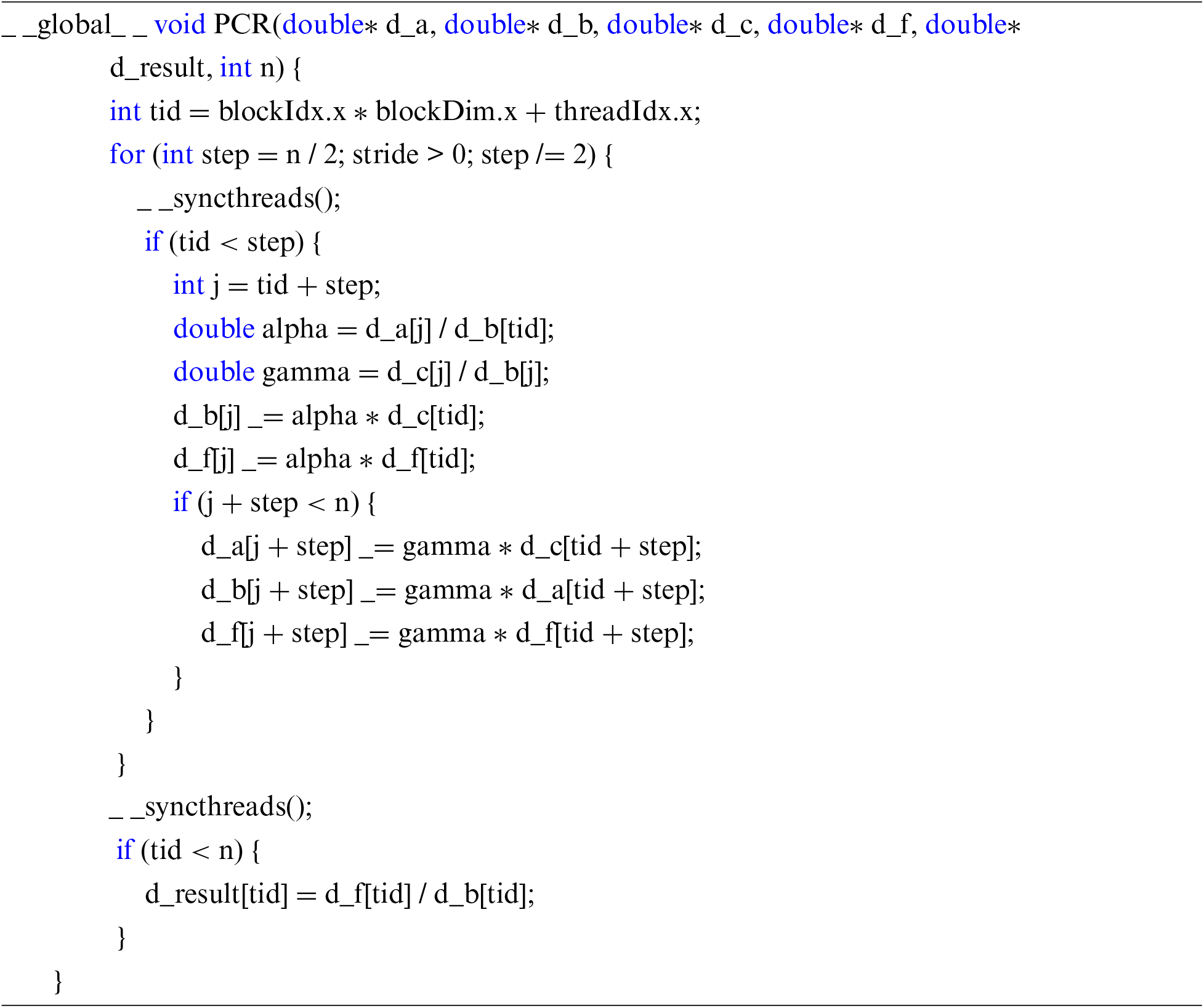
Initially, we define the kernel execution parameters. The number of blocks corresponds to the size of the system, with each individual system being assigned to one block. All variables are stored in memory using a Double-Precision Floating Point format. We utilize five global arrays for data storage: three for the tridiagonal matrix elements, one for the right-hand side, and one for the solution vector. The shared memory allocated tridiagonal system amounts to n * 5 * size of(double) bytes. During the forward phase of the algorithm, log2(n/2) steps are executed. All five arrays are shared memory arrays, with data loaded from global memory. The step begins at 1 and doubles with each subsequent step of the algorithm, while the number of active threads is halved at each stage. At the start of the backward phase, we solve a system of equations derived from two equations at the final step of the forward phase. We then apply the algorithm to determine all other unknowns in log2(n/2) steps.

The kernel function is shown below in Listing 3.1.

By executing the kernel function log_2n times, n is the number of equations, we find all the unknowns of a three-diagonal system after that we will copy calculated data yi from the device to the host.

3.2 Experimental Results

To evaluate the program’s performance, we utilized a personal computer featuring an eight-core Intel Core i7-9800X processor, running at a clock speed of 3.8 GHz, coupled with 64 GB of RAM. Additionally, the system was equipped with an Nvidia RTX 2080 graphics card containing 4352 cores and 8 GB of video memory. The operating system employed was Windows 10. Both parallel and sequential algorithms were implemented using the C++ programming language. Key parameters for the problem were configured as follows: mesh size (N) maintained uniformity in both directions with a step size of Δx=Δy=0.05, a time step of Δt = 0.005, and a total simulation time of 0.5. Consequently, the number of time iterations amounted to 100. The mesh size was chosen as a power of two plus one, and the block size was determined based on the value of N and the GPU’s processing capabilities, imposing limitations on the grid size. In Table 2, we report the execution times in seconds for serial (CPU time) and CUDA (GPU time) implementation of the parallel cyclic reduction method to the problem (1)–(4) together with the values of the speedup computed as the ratio. The calculation results in the table indicate a moderate speedup for small domains up to a size of 1024×1024, but a pronounced increase occurs when working with larger domains. This is because large domains generate a significant computational load, which can be efficiently parallelized across multiple GPU processors. The parallelism provided by the GPU plays a key role in achieving speedup, and larger domains naturally provide greater parallel processing capabilities.

4  Conclusions and Future Work

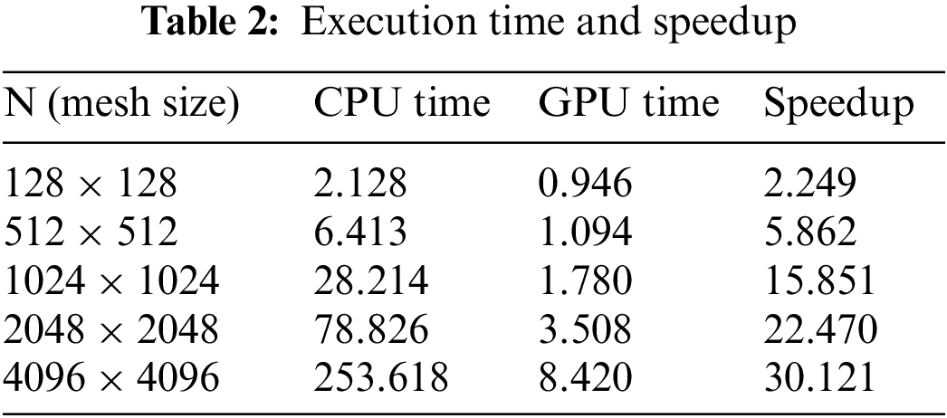
In this work, we proposed a parallel numerical solution to the two-dimensional acoustic wave equation in heterogeneous media. We used a fully implicit finite difference scheme with a parallel cyclic reduction method. The implemented parallel algorithms were run on a GPU, and the computational results were subjected to comparative analysis. As the results from Table 2 show, our parallel implementations are 2–30 times faster than the sequential algorithm. Despite these significant performance improvements, our work has several limitations. The scalability of the current implementation may be hindered by communication overheads and synchronization requirements when scaling to larger GPU clusters. Additionally, the performance gains are heavily dependent on the specific GPU architecture used, which may limit the generalizability of our results across different hardware configurations.

In future research plans, we intend to improve our parallel algorithms for GPU clusters. Specifically, we aim to address the identified limitations by exploring more efficient communication strategies, optimizing the algorithms for various GPU architectures, and developing techniques to better handle complex boundary conditions and large-scale problems.

Acknowledgement: The authors express their gratitude to the anonymous reviewer for their insightful revision suggestions.

Funding Statement: This research was funded by the Committee of Science of the Ministry of Science and Higher Education of the Republic of Kazakhstan (Grants No. AP14972032). NT is also supported by the Beatriu de Pinós programme and by AGAUR (Generalitat de Catalunya) grant 2021 SGR 00087.

Author Contributions: The authors confirm their contribution to the paper as follows: study conception, visualization, and methodology: Arshyn Altybay; analysis and interpretation of results: Niyaz Tokmagambetov; draft manuscript preparation: Arshyn Altybay. All authors reviewed the results and approved the final version of the manuscript.

Availability of Data and Materials: The authors declare that the data in the article will be provided as needed.

Ethics Approval: Not applicable.

Conflicts of Interest: The authors declare that they have no conflicts of interest to report regarding the present study.

References

1. Heiner I. Computational seismology: a practical introduction. Oxford, UK: Oxford University Press; 2017. [Google Scholar]

2. Shearer PM. Introduction to seismology. Cambridge, UK: Cambridge University Press; 2019. [Google Scholar]

3. Aki K, Richards PG. Quantitative seismology. Sausalito, CA, USA: University Science Books; 2002. [Google Scholar]

4. Kelly KR, Ward RW, Treitel S, Alford EM. Synthetic seismograms: a finite difference approach. Geophysics. 1976;41(1):2–27. doi:10.1190/1.1440605. [Google Scholar] [CrossRef]

5. Cohen G, Joly P. Construction and analysis of fourth-order finite difference schemes for the acoustic wave equation in non-homogeneous media. SIAM J Numer Anal. 1996;4:1266–302. [Google Scholar]

6. Takeuchi N, Geller RJ. Optimally accurate second order time-domain finite difference scheme for computing synthetic seismograms in 2-D and 3-D media. Phys Earth Planet Inter. 2000;119(1–2):99–131. doi:10.1016/S0031-9201(99)00155-7. [Google Scholar] [CrossRef]

7. Chen JB. High-order time discretizations in seismic modelling. Geophysics. 2007;72(5):115–22. doi:10.1190/1.2750424. [Google Scholar] [CrossRef]

8. Liao W. On the dispersion, stability and accuracy of a compact higher-order finite difference scheme for 3D acoustic wave equation. J Comput Appl Math. 2014;270(1):571–83. doi:10.1016/j.cam.2013.08.024. [Google Scholar] [CrossRef]

9. Liao W, Yong P, Dastour H, Huang J. Efficient and accurate numerical simulation of acoustic wave propagation in a 2D heterogeneous media. Appl Math Comput. 2018;321(4):385–400. doi:10.1016/j.amc.2017.10.052. [Google Scholar] [CrossRef]

10. Li K, Liao W. An efficient and high accuracy finite-difference scheme for the acoustic wave equation in 3D heterogeneous media. J Comput Sci. 2020;40:101063. doi:10.1016/j.jocs.2019.101063. [Google Scholar] [CrossRef]

11. Wu M, Jiang Y, Ge Y. An accurate and efficient local one-dimensional method for the 3D acoustic wave equation. Demonstratio Math. 2022;55(1):528–52. doi:10.1515/dema-2022-0148. [Google Scholar] [CrossRef]

12. Landinez G, Santiago R, Fabio DL. First steps on modelling wave propagation in isotropic-heterogeneous media: numerical simulation of P-SV waves. Eur J Phys. 2021;42(6):1–26. doi:10.1088/1361-6404/ac18cf. [Google Scholar] [CrossRef]

13. Virieux J. P-SV wave propagation in heterogeneous media: velocity stress finite difference method. Geophysics. 1986;51(4):889–901. doi:10.1190/1.1442147. [Google Scholar] [CrossRef]

14. Zhang J, Liu T. P-SV-wave propagation in heterogeneous media: grid method. Geophys J Int. 2010;136(2):431–8. [Google Scholar]

15. Tsvankin I, Grechka V. Seismology of azimuthally anisotropic media and seismic fracture characterization. Tulsa: Society of Exploration Geophysicists; 2011. [Google Scholar]

16. Masson Y, Virieux J. P-SV wave propagation in heterogeneous media: velocity-stress distributional finite-difference method. Geophysics. 2023;88(3):1–92. [Google Scholar]

17. Klockner A, Warburton T, Bridge J, Hesthaven JS. Nodal discontinuous Galerkin methods on graphics processors. J Comput Phys. 2009;228(21):7863–82. [Google Scholar]

18. Bell N, Garland M. Efficient sparse matrix-vector multiplication on CUDA. Santa Clara, CA, USA: NVIDIA Technical Report; 2008. [Google Scholar]

19. Mehra R, Raghuvanshi N, Savioja L, Lin M, Manocha D. An efficient GPU-based time domain solver for the acoustic wave equation. Appl Acoust. 2012;73:83–94. [Google Scholar]

20. Weiss RM, Shragge J. Solving 3D anisotropic elastic wave equations on parallel GPU devices. Geophysics. 2013;78(2):1–9. [Google Scholar]

21. Lastra M, Castro MJ, Urena C, Asuncion M. Efficient multilayer shallow-water simulation system based on GPUs. Math Comput Simul. 2018;148:48–65. doi:10.1016/j.matcom.2017.11.008. [Google Scholar] [CrossRef]

22. Altybay A, Ruzhansky M, Tokmagambetov N. A parallel hybrid implementation of the 2D acoustic wave equation. Int J Nonlinear Sci Numer Simul. 2020;21(7–8):821–7. doi:10.1515/ijnsns-2019-0227. [Google Scholar] [CrossRef]

23. Peaceman DW, Rachford HH. The numerical solution of parabolic and elliptic differential equations. J Soc Ind Appl Math. 1955;3(1):28–41. doi:10.1137/0103003. [Google Scholar] [CrossRef]

24. Douglas JJ, James EG. A general formulation of alternating direction methods. Numer Math. 1964;6(1):428–53. doi:10.1007/BF01386093. [Google Scholar] [CrossRef]

25. Douglas J, Rachford HH. On the numerical solution of heat conduction problems in two and three space variables. Trans Am Math Soc. 1956;82(2):421–89. doi:10.1090/S0002-9947-1956-0084194-4. [Google Scholar] [CrossRef]

26. Lees M. Alternating direction methods for hyperbolic differential equations. J Soc Ind Appl Math. 1962;10(4):610–6. doi:10.1137/0110046. [Google Scholar] [CrossRef]

27. Wei X, Rao C, Chen S, Luo W. Numerical simulation of anti-plane wave propagation in heterogeneous media. Appl Math Lett. 2023;135:108436. doi:10.1016/j.aml.2022.108436. [Google Scholar] [CrossRef]

28. Wei X, Luo W. 2.5D singular boundary method for acoustic wave propagation. Appl Math Lett. 2021;112(4):106760. doi:10.1016/j.aml.2020.106760. [Google Scholar] [CrossRef]

29. Coyle AJ, Ayub Md, Boettger D, Cervera MA, MacKinnon AD. Impact of internal waves on underwater acoustic propagation. J Acoust Soc Am. 2023;154(4):A81. [Google Scholar]

30. Zeng Q, Liu S, Tang L, Li Z. Theoretical and numerical study on transient acoustic wave propagation across ice layers in the Arctic Ocean. J Acoust Soc Am. 2024;155(5):3132–43. doi:10.1121/10.0025982. [Google Scholar] [PubMed] [CrossRef]

31. Luis MP, Juan LF. Generalization of Snell’s Law for the propagation of acoustic waves in elliptically anisotropic media. AIMS Math. 2024;9(6):14997–5007. doi:10.3934/math.2024726. [Google Scholar] [CrossRef]

32. Xue Y, Yue L, Kang X, Yuxing L, Liu C. Investigation on propagation mechanism of leakage acoustic waves in gas-liquid stratified flow. Ocean Eng. 2022;266(2):112962. doi:10.1016/j.oceaneng.2022.112962. [Google Scholar] [CrossRef]

33. von Neumann J, Richtmyer RD. A method for the numerical calculation of hydrodynamic shocks. J Appl Phys. 2004;21(3):232–7. doi:10.1063/1.1699639. [Google Scholar] [CrossRef]

34. Mishra S, Svard M. On stability of numerical schemes via frozen coefficients and the magnetic induction equation. BIT Numer Math. 2010;50(1):85–108. doi:10.1007/s10543-010-0249-5. [Google Scholar] [CrossRef]

35. Vetterling WT, Teulokshy SA, Press WH, Flannery BP. Numerical recipes: the art of scientific computing. Cambridge, UK: Cambridge University Press; 1985. [Google Scholar]

36. Hockney RW, Jesshope C. Parallel computers. Bristol, UK: Adam Hilger; 1981. [Google Scholar]

37. Hockney RW. A fast direct solution of Poisson’s equation using Fourier analysis. J ACM. 1965;12(1):95–113. doi:10.1145/321250.321259. [Google Scholar] [CrossRef]

38. Altybay A, Darkenbayev D, Mekebayev N. Numerical simulation and GPU computing for the 2D wave equation with variable coefficient. Int J Simul Process Model. 2023;20(4):298–305. doi:10.1504/IJSPM.2023.138584. [Google Scholar] [CrossRef]

39. NVIDIA TURING GPU ARCHITECTURE. Available from: https://www.nvidia.com/content/dam/en-zz/Solutions/design-visualization/technologies/turing-architecture/NVIDIA-Turing-Architecture-Whitepaper.pdf. [Accessed 2018]. [Google Scholar]

40. Zhang Y, Cohen J, Owens J. Fast tridiagonal solvers on the GPU. ACM Sigplan Notices. 2010;45(5):127–36. doi:10.1145/1837853.1693472. [Google Scholar] [CrossRef]