
 Submit a Paper
 Propose a Special lssue
 Open Access
ARTICLE
Advancements in Numerical Solutions: Fractal Runge-Kutta Approach to Model Time-Dependent MHD Newtonian Fluid with Rescaled Viscosity on Riga Plate
1 Department of Mathematics and Sciences, College of Humanities and Sciences, Prince Sultan University, Riyadh, 11586, Saudi Arabia
2 Department of Mathematics, Air University, PAF Complex E-9, Islamabad, 44000, Pakistan
* Corresponding Author: Muhammad Shoaib Arif. Email:
(This article belongs to the Special Issue: New Trends on Meshless Method and Numerical Analysis)
Computer Modeling in Engineering & Sciences 2024, 141(2), 1213-1241. https://doi.org/10.32604/cmes.2024.054819
Received 08 June 2024; Accepted 12 August 2024; Issue published 27 September 2024
 View Full Text
 Download PDF
Abstract
Fractal time-dependent issues in fluid dynamics provide a distinct difficulty in numerical analysis due to their complex characteristics, necessitating specialized computing techniques for precise and economical solutions. This study presents an innovative computational approach to tackle these difficulties. The main focus is applying the Fractal Runge-Kutta Method to model the time-dependent magnetohydrodynamic (MHD) Newtonian fluid with rescaled viscosity flow on Riga plates. An efficient computational scheme is proposed for handling fractal time-dependent problems in flow phenomena. The scheme is comprised of three stages and constructed using three different time levels. The stability of the scheme is shown by employing the Fourier series analysis to solve scalar problems. The scheme’s convergence is guaranteed for a time fractal partial differential equations system. The scheme is applied to the dimensionless fractal heat and mass transfer model of incompressible, unsteady, laminar, Newtonian fluid with rescaled viscosity flow over the flat and oscillatory Riga plates under the effects of space- and temperature-dependent heat sources. The first-order back differences discretize the continuity equation. The results show that skin friction local Nusselt number declines by raising the coefficient of the temperature-dependent term of heat source and Eckert number. The numerical simulations provide valuable insights into fluid dynamics, explicitly highlighting the influence of the temperature-dependent coefficient of the heat source and the Eckert number on skin friction and local Nusselt number.Keywords
Nomenclature
| Horizontal components of velocity | |
| Cartesian co-ordinate | |
| Electrical conductivity of the fluid | |
| Kinematic viscosity | |
| Density of fluid | |
| Concentration of fluid | |
| Current density | |
| Specific heat capacity | |
| Width of the magnet and electrodes | |
| Reaction rate | |
| Reaction rate parameter | |
| Newtonian fluid with rescaled viscosity parameter | |
| Magnetic parameter | |
| Prandtl number | |
| Reynolds number | |
| Electrode’s width and the magnets | |
| Dimensionless parameter | |
| Dimensionless horizontal and vertical components of velocity | |
| Dimensionless temperature | |
| Vertical components of velocity | |
| Cartesian co-ordinate | |
| Temperature of fluid | |
| Temperature of fluid at the wall | |
| Ambient temperature of the fluid | |
| Concentration on the wall | |
| Ambient concentration | |
| Magnetization of the magnet | |
| Strength of imposed transverse magnetic field | |
| Thermal diffusivity | |
| Dynamic viscosity | |
| Hartmann number | |
| Eckert number | |
| Modified Hartmann number | |
| Schmidt number | |
| Mass diffusivity | |
| Dimensionless parameter | |
| Dimensionless coordinates | |
| Dimensionless concentration |
Fluid dynamics have long enthralled scientific investigation due to its complicated and sophisticated interplay of forces. Researchers have recently focused more on solving the problems of time-dependent phenomena in fluid dynamics, thanks to improvements in numerical approaches and a spike in processing power [1]. Fractal time-dependent problems are incredibly fascinating since they present unique difficulties for numerical analysis due to their complexity and self-repeating patterns. A unique computational approach is presented in this study to tackle the difficulties of fractal time-dependent issues and contribute to the improvement of numerical solutions in fluid dynamics [2]. We are particularly interested in the area where Newtonian fluid dynamics meets magnetohydrodynamics (MHD), where the behaviour of time-dependent fluids affected by magnetic fields is crucial. Another new development in geometry is ‘fractal geometry’, which helps to create a masterpiece of the flow pattern and its general attributes on several scales [3]. This can significantly improve the results and the way of modelling behind employing complexities and methods of fractal view.
The purpose of the current study was to verify the complexity of flow by comparing it to other fractals. Fractals in mathematics are geometric appearances that can be divided into pieces and cut out, where each piece’s reduction is that very essence known as fractality. We need to adjust these linear and non-linear differential equations that give solutions of flow fields with a set of calculations so it can quickly figure out the different patterns of flow fields over several times and space scales. We use the Fractal Runge-Kutta Method to solve the problem. It is an efficient way to find an approximate answer, whereas when we use the method in flow, it successfully displays the flow details at different times and scales. When we try to study the dynamics of a time-dependent fractal MHD Newtonian fluid with rescaled viscosity over the Riga plate, a moving surface is used as the wall [4]. Since identifying the flow detail and heat transfer is not a simple problem, we also needed the terminal of mathematical methods to derive the results. Therefore, we used a fractal method to model the problem. The comparison with fractals as and when needed can help us determine the flow pattern’s complexity. In the modern techniques of geometry or the field of fluid flow analysis, the employment of fractal theory can improve the predictability of the pattern of flow behaviour. In the study, we see the use of geometry in the case of a dynamics problem [5].
Flows similar at different time scales can reflect the complexity of the fractal structure of a flow. There are various ways to make a computer do fractal analysis, and various computer programs are available on the internet to help us perform that task on our own. One such famous fractal is far from us to find a set of complex roots of a polynomial. We needed an efficient way to get a target result with a close approach; thus, we used a completely modified approach, Runge-Kutta. We can infinitely approximate the error of the flow field into a particular area and then fix those results and validate them from our fractal comparison.
The Fractal Runge-Kutta Method is a version of the Runge-Kutta scheme and is a very efficient way to solve differential equations that show fractal characteristics. Traditionally, the equations to be solved are essentially third-, fourth-, and fifth-order differential equations. Hence, a suitable fractal point is to be achieved, and then the differential equations are solved to get a particular result. That’s where Fractal Runge Kutta differs from traditional. It comes up with a target point and the error value to get an exact result value that is as close as possible to the append error. And that’s what we needed to solve the problem. It allows the accurate portrayal of physical phenomena. To summarise, Fractals can assist us in many fractals when we get stuck. Solving difficult problems yields constants-based fractal calculations that allow us to draw quick conclusions and retain seemingly impossible answers. These fractals would account for many mathematical interpretations while we analyze the problem through different patterns. When we try to see what is happening in the flow (when the flow field turns out to be very subtle), we find connecting these Roman coefficients to form a Pythagorean Theorem and then adjusting the results as much as possible.
A boundary layer in fluid dynamics is a thin layer that has been researched in theory in fluid dynamics. It’s a thin layer of each phase or a boundary layer in each phase. It has been around for more than a century. It started when Ludwig Prandtl developed it in 1904. The boundary layer has powerful effects on the motion of fluids and represents their characteristics. Hence, studying a Riga plate is an essential dynamic phenomenon [6]. It can be stated as a fluid layer that flows directly over a surface, including shear flow. Researchers have conducted studies to explore the nature of the flow of the layers in various forms of geometry, elongated shape, and horizontal plates [7], Read Less vertical plates, being infinite in length [8], stretching sheets [9], and Read Less wedges [10]. A novel device called the Riga plate has been developed to minimize skin friction in movement [11]. The electromagnetic properties of the Riga plate can be utilized to study the effects of thermal radiation and viscous dissipation when the plate is submerged in a setup by positioning electrodes on it. Research on this geometry has lately gathered steam in the 21st Century, despite Gailitis and Lielausis introducing this plate in 1961 [12]. Using the Cattaneo Christov model [13], we studied the impact of radiation and chemical reactions on Darcy Forchheimer flow, focusing on a Williamson fluid passing over a Riga plate. Later, Reyaz et al. [14] used both numerical methods to analyze the data.
In a study [14], the Zakians method was employed to analyze the flow behaviour near a Riga plate under the influence of a magnetic field. The findings suggested that the presence of the Riga plate impacts the velocity. Particle deposition effects in Casson-type hybrid nanofluid flow over a Riga plate were investigated in another study by [15] utilizing techniques like the Runge-Kutta Fehlberg method. Additionally, using analysis [16]. They have examined the stagnation point flow of a hybrid nanofluid across a Riga plate. Furthermore, in their paper, Loganathan et al. [17] examined how variable chemical reactions affect Casson fluid flow over a Riga plate in a medium. The buoyancy-driven Casson fluid flow from a vertical wavy surface in the presence of a magnetic field is studied numerically in the proposed study [18], which also provides a quantitative and qualitative assessment of the underlying heat transport in the free convective regime.
Computer networking, dynamics, control theory, and biology have all seen a rise in the use of fractional calculus. Analyzing memory effects is made easier using this tool. Fluid problems are now being approached using methods, a new trend [19]. Different mathematicians have defined derivatives with and without kernels [20]. Atangana Baleanu derivative is one example of such a derivative [21]. When dealing with nonlocal behaviour and equations with non-singular kernels, this derivative proves to be helpful [22]. It assists in addressing real-world issues such as heat and mass transfer, electrical circuits, image processing, and the adverse effects of chemotherapy in cancer treatment [23]. The Casson fluid flow alongside a plate was studied by Tassaddiq et al. [24] using a fractional approach. Using the Laplace transform and Zakians algorithm, they solved transformed equations.
Shah and colleagues examined the Atangana-Baleanu derivative’s utilization in the flow analysis between plates [25] and cylinders [26]. The study in [27] investigated the flow behaviour of nanofluids containing spherical-shaped Molybdenum Disulphide nanoparticles using an AB derivative. Saqib et al. [28] examined the CNT nanofluid’s channel flow properties with CMC as the base fluid employing an AB derivative. This numerical study [29] investigated the fractional viscoelastic fluid model with unstable convection on an inclined plane through a Forchheimer medium. This paper [30] focuses on developing a fractional explicit-implicit numerical method for solving time-dependent partial differential equations. In their work, Nawaz et al. [31] proposed a third-order numerical approach for solving fractional partial differential equations. The initial explicit stage can rapidly converge, while the subsequent implicit stage is responsible for expanding the stability region.
Numerous research efforts have been devoted to exploring the practical applications of nanofluids in heat transfer studies. Nanofluids are essentially solutions comprised of a fluid infused with nanoparticles synthesized in laboratories to create an innovative solution that enhances overall fluid behaviour for improved outcomes. While work on these fluids has been ongoing since the 1990s, Choi first introduced and coined the term “nanofluids” in 1995 [32]. Using far nanofluids has yielded promising outcomes in various disciplines, from engineering to healthcare. The consequences of nanofluid flow in geometries have been the subject of much mathematical discussion; these findings have significant practical ramifications.
Offer insights into the utilization of nanoparticles in the base fluid. Magnetite nanoparticles exhibit potential in applications and research [33]. They prove helpful for diagnosing and treating diseases. Due to their potential in applications, researchers have devoted significant attention to magnetite nanoparticles in their studies for several decades. The features of these nanoparticles make them widely used in treatment. The effect of conductivity on magnetite nanofluid-based sheets subjected to shrinkage and stretching was studied by [34]. In their paper, Seth et al. [35] discussed ferrofluid flow over a plate with oscillating behaviour.
In this context, while traditional Runge-Kutta (RK) methods effectively solve equations, they often face challenges when capturing the complex and non-linear dynamics of time fractal MHD Newtonian fluid with rescaled viscosity flows over Riga plates. This is where Fractal Runge-Kutta (FRK) methods emerge as an alternative. FRK methods utilize the concept of calculus, extending the idea of differentiation and integration beyond numbers. Complex physical systems frequently exhibit fractal time’s complexity and irregular structure, which exemplifies it. By incorporating these derivatives into the RK framework, FRK methods demonstrate improved accuracy and stability, especially when dealing with highly non-linear and singular problems.
The previous studies on flow and heat transfer on stretching sheets have captured the attention of scholars across fields. It holds significance in polyamide production due to advancements in polymers. With the idea of moving planes and velocities that change the distance from fixed locations on a sheet in a linear fashion, Crane [36] investigated these concepts. Many researchers have recently employed Newtonian fluids for heat and mass transfer [37,38]. Nadeem et al. [39] investigated second-grade fluids’ time-dependent stretching behaviour. The paper by Majeed et al. [40] suggested using the suction of stretching surfaces to study the flow of non-Newtonian fluids. The References [41,42] described a new class of exact solutions to the Oberbeck-Boussinesq equations that describe an incompressible fluid.
This study is unique because it takes an interdisciplinary approach, applies the Fractal Runge-Kutta Method, develops an efficient computational scheme, investigates fractal time-dependent fluid dynamics, and uncovers valuable insights into fluid dynamics phenomena. All of these things add up to a more advanced numerical solution to complicated fluid dynamic problems, which in turn opens up new possibilities for study and development in the area:
1. A new computational approach is used to solve fractal time-dependent fluid dynamics problems. The Fractal Runge-Kutta Method models time-dependent MHD Newtonian fluid with rescaled viscosity on Riga plates.
2. A three-stage computational approach using three-time levels is proposed. This comprehensive approach captures the complexity of fractal time-dependent problems to provide a sophisticated knowledge of fluid dynamics.
3. Fourier series analysis of scalar issues proves the computing scheme’s stability. Moreover, a convergence analysis for a time-dependent fractal partial differential equations system ensures the numerical method’s dependability and correctness.
4. The computational approach is applied to a dimensionless fractal model of incompressible, unstable, laminar Newtonian fluid with rescaled viscosity over flat and oscillatory Riga plates. For practicality, space- and temperature-dependent heat sources are included in the numerical simulations.
5. We present a powerful computational technique for fractal time-dependent fluid dynamics problems. We ensure numerical solution accuracy and efficiency using a scheme with three-time levels and rigorous stability analysis.
The Riga plate geometry was selected for our investigation due to theoretical and practical considerations of fluid dynamics. What follows is an outline of our decision-making procedure, along with some examples of its potential applications:
1. Theoretical Considerations: The Riga plate design is straightforward and analytically understandable for fluid flow studies. Its primary and adjustable geometry allows for studying fundamental fluid dynamics topics, making it a popular choice for theoretical and computational fluid mechanics investigations. We can use the Riga plate’s simple geometry to learn about time-varying fluid dynamics in controlled conditions.
2. Practical Applications: Despite its theoretical simplicity, the Riga plate geometry has extensive practical applications across various industries. For example:
a. Heat Exchangers: The Riga plate geometry finds utility in heat exchangers, which transfer heat from one fluid to another using a series of flat or oscillating plates. A comprehensive comprehension of the fluid dynamics across Riga plates is necessary for systems to achieve optimal heat transfer efficiency.
b. Aerospace Engineering: Regarding aerospace applications, the Riga plate geometry is a common feature in the design of airfoils and wings. The fluid flow characteristics over these surfaces are essential in determining the aerodynamic performance. Studying fluid dynamics over Riga plates can provide valuable insights into airflow behaviour, which can help improve efficiency and stability in aerospace systems.
Therefore, the article focuses on advancing and implementing a particular FRK technique to investigate the time fractal MHD Newtonian fluid dispersion with rescaled viscosity flows on Riga plates. We expect that this method will offer valuable information regarding the correlation between the Newtonian characteristics of the fluid, magnetic fields, and fractal time scales. These insights can be applied in various sectors, including optimizing heat transfer processes, regulating flow instabilities, and creating innovative material coatings.
2 The Fractal Numerical Scheme
The fractal scheme is a numerical method consisting of three stages that can be used to discretize time-dependent PDEs. Any finite difference discretization or other scheme can be employed for spatial discretization. Before proposing a scheme, the whole domain is divided into small subintervals with endpoints called grid points. The solution will be found at each grid point using the proposed scheme except at those where boundary conditions are given. The main advantage of using the proposed scheme is that it does not require linearization or any other iterative scheme. The scheme is employed to follow time fractal partial differential equations.
where
where
The first stage of the scheme is:
The first stage (1) finds the solution of Eq. (1) at an arbitrary time level. This stage (1) can also be called as predictor stage. The second stage of the proposed scheme can be written as:
This stage (4) is also a predictor stage that finds the solution of the fractal partial differential equation at an arbitrary time level. It also utilizes the solution computed from the first predictor stage. The third stage of the proposed scheme can be articulated as:
where
Now, substituting the first predictor stage (3) into the second predictor stage (4) yields:
By using Eqs. (3) and (6) into corrector stage (5), it yields:
Expanding
By substituting fractal Taylor series expansion of
By equating coefficients of
Solving Eq. (10) yields:
Therefore, the proposed fractal scheme for Eq. (1) with second-order central space discretization is given as:
where
Let
The Fourier series analysis exists in the literature to find the stability conditions of partial differential equations. The scheme can be applied to non-linear PDEs, but it estimates the exact stability conditions in this case. For non-linear differential equations, equations are linearized first, and then this criterion is employed. This criterion is based on some transformations that convert the different equations into trigonometric equations with the involvement amplitude of waves. To apply this criterion, consider the following transformations:
where
Simplifying Eq. (19) yields:
Re-write Eq. (20) as:
Let
Similarly, substituting corresponding transformations from (18) into the second stage of the proposed scheme gives:
By using Eq. (22) in Eq. (23), it gives:
Similarly, the following equation can be obtained by applying suitable transformations from (18) into the third stage of the proposed scheme (17):
where
Upon substituting Eqs. (22) and (24) into Eq. (25) that gives:
Eq. (26) can be written as:
where is
The amplification factor, in this case, is:
If the step size and

Figure 1: Stability regions
The next task is to provide convergence with the proposed scheme. For doing so, consider the system of fractal partial differential equations as follows:
where
Theorem 1: The proposed scheme (30)–(32) converges conditionally for Eq. (29).
Proof: Let the first stage of the exact scheme for (29) be:
Subtracting Eq. (30) from Eq. (33) and considering:
The resulting equation is:
Applying the norm on both sides of Eq. (34) and using triangle inequality yields:
where
The second stage of the scheme is expressed as:
Similarly, the following inequality can be obtained by subtracting Eq. (31) from Eq. (36):
Let the third stage of the exact scheme be:
Similarly, subtracting the proposed scheme’s third stage from the exact scheme’s third stage and applying the norm yields inequality.
where
Re-write inequality (40) as:
where
Let
Since
Suppose
If this continued, then for finite n:
when
Consider laminar, incompressible, two-dimensional, unsteady, Newtonian fluid with rescaled viscosity flow over flat, oscillatory sheets. Let

Figure 2: Geometry of the problem
Description of the Geometry:
1. Riga Plate Configuration (Left part of Fig. 2): The Riga plate is represented with alternating positive and negative electrodes placed along the
2. Coordinate System: The
3. Flow and Boundary Layers (Right part of Fig. 2): The fluid flow is initiated due to the sudden movement of the plate along the
A model of Casson fluid has been presented in [43], and here, the modified Casson model with space and temperature-dependent heat source is presented. The flow can be described using the governing equations:
Subject to the initial and boundary conditions:
where
The problem formulation incorporates boundary conditions that accurately represent the physical mechanics of fluid flow over the Riga plates. These conditions take into account factors such as temperature and concentration gradients, as well as the impacts of magnetization and heat sources. Below are the comprehensive boundary conditions together with their corresponding physical mechanisms:
1. Initial Condition: At
2. Boundary Conditions on the Plate Surface
3. Boundary Conditions along with the Leading Edge
4. Far-Field Conditions
These conditions ensure a realistic representation of the initial state and the interactions at the boundaries, providing a comprehensive framework for analyzing the fluid dynamics problem.
Into Eqs. (46)–(50), the dimensionless equations are obtained as:
With dimensionless initial and boundary conditions:
where
The time fractal model is expressed as:
with the same initial and boundary conditions (56) as the classical model.
The skin friction coefficients, local Nusselt number, and Sherwood number are precisely defined as:
where
Applying transformations (51) to Eqs. (61)–(63) yields dimensionless skin friction coefficients, local Nusselt numbers, and Sherwood numbers:
Justification for Time Fractal Model: Complex features in fluid dynamics, especially in a Newtonian fluid with rescaled viscosity fluid flow over a plate, inspired the development of a temporal fractal model. Even while classical models (52)–(55) have been around for a while, we can capture more temporal subtleties with the time fractal model (57)–(60). A flexible framework for modelling anomalous diffusion or other non-traditional time-dependent behaviours in the system can be provided by the fractal derivative in time, which is represented by the parameter
Physical Meaning of
Comparison with Classical Model (52)–(55): There is a double benefit to including both the traditional (52)–(55) and fractal (57)–(60) models. We can demonstrate the time fractal model’s benefits in capturing extra-temporal complexities by comparing it to the classical model, which serves as a benchmark. Our goal in comparing the two models is to show how the fractal model is more sensitive and powerful in our particular fluid dynamics case.
Assumption and Limitations: This study proposes certain assumptions in order to simplify the modelling of time-dependent magnetohydrodynamic (MHD) Newtonian fluid flow with rescaled viscosity on Riga plates using the Fractal Runge-Kutta Method. First, it assumes Newtonian, incompressible, laminar, two-dimensional fluid behaviour, simplifying real-world fluid behaviour. The study idealizes flow commencement by assuming a sudden plate movement. It also assumes the plate’s temperature and concentration exceed the surrounding environment, creating continuous boundary conditions. The Riga plate, with alternating electrodes and permanent magnets, models electromagnetic effects, but other designs may not. Internal heat generation depends on space and temperature, although the parameters may not cover all circumstances. The chemical reaction is modelled with a defined reaction rate and a simplified mechanism, which may not capture more complex reactions.
The study has significant limitations. The research is limited to high Reynolds number settings with severe turbulence since it does not account for turbulent flow. Practical applications may involve more sophisticated geometries than flat and oscillating sheets. Although efficient, the proposed computational technique may be computationally expensive for very fine time increments or large-scale issues, limiting its usefulness. The validation of the scheme is based on specific examples, suggesting it has to be expanded to include more complex fluid behaviours and scenarios. These limitations limit the study’s conclusions and indicate topics for further research to handle more complicated or variable conditions.
An explicit computational scheme that finds the solution of fractal partial differential equations in three stages is proposed. The first two stages of the schemes are predictor stages that find the solutions at arbitrary time levels. So, the time from
• Newtonian fluid with rescaled viscosity parameter
• Hartmann number
• Modified Hartman number
• Eckert number
• Coefficients of space and temperature-dependent terms of internal heat generation
• Schmidt number
• Reaction rate parameter
The values of parameters depend on the convergence of the scheme. Any parameter value can be chosen if the scheme meets the stability condition. However, for higher values of the parameters, the step size in time must be appropriately chosen to get a stable solution. Meeting the stability condition, in this case, makes the scheme computationally expensive.
Fig. 3 shows the effect of the Newtonian fluid with rescaled viscosity parameter in the velocity profile. The velocity decays by raising the Newtonian fluid with a rescaled viscosity parameter. Since the coefficient of diffusion declines by rising Newtonian fluid with rescaled viscosity parameters, the diffusion process becomes slow, and the velocity profile declines. Fig. 4 shows the effect of Hartmann’s number velocity profile. The velocity profile declines when the Hartmann number is increased. The velocity profile declines since the Lorenz force grows by rising Hartmann number, which leads to increased resistance in the fluid flow. Fig. 5 displays the variation of the modified Hartmann number on the velocity profile. The velocity profile grows by enhancing the modified Hartmann number.

Figure 3: Effect of Newtonian fluid with rescaled viscosity parameter on velocity profile using

Figure 4: Effect of Hartmann number on velocity profile using

Figure 5: Effect of modified Hartmann number on velocity profile using
The impact of the Eckert number on the temperature profile is depicted in Fig. 6. Temperature grows as the Eckert number enhances. The Eckert number is the ratio of kinetic energy to enthalpy. By raising the Eckert number, the internal friction of the fluid increases, and the temperature gradient is not the only factor that raises the temperature. It also depends on dissipation due to internal friction. Therefore, increasing the Eckert number increases self-heating, so the temperature profile grows. Figs. 7 and 8 show the effect of coefficients of space and temperature-dependent terms of internal heat generation. Temperature profile rises by augmenting both coefficients of space and temperature-dependent terms of heat source. Since heat generation increases due to the enhancement of both coefficients, this heat rise leads to growth in the temperature profile. Fig. 9 illustrates the impact of the Schmidt number on the concentration profile. The concentration profile decreases as the Schmidt number increases. Increasing the Schmidt number causes a decrease in mass diffusivity, resulting in a decay in the concentration profile. Fig. 10 illustrates the relationship between the concentration profile and the response rate parameter’s fluctuation. The concentration profile declines by raising the reaction rate parameter. The formation or breaking of chemical bonds between atoms is due to chemical reactions in which reactants are converted into products, leading to a decline in the concentration profile.

Figure 6: Effect of Eckert number on temperature profile using

Figure 7: Effect of the coefficient of the space-dependent term of heat source on temperature profile using

Figure 8: Effect of the coefficient of the temperature-dependent term of heat source on temperature profile using

Figure 9: Effect of the Schmidt number on concentration profile using

Figure 10: Effect of reaction rate parameter on concentration profile using
The effect of the modified Hartmann number and Newtonian fluid with rescaled viscosity parameter on the skin friction coefficient is displayed in Fig. 11. The skin friction coefficient rises as the modified Hartmann number and Newtonian fluid with rescaled viscosity parameter grow. Since the velocity profile increases by raising the modified Hartmann number, friction at the plate grows, enhancing the skin friction coefficient. Fig. 12 displays the variation of the coefficient of temperature-dependent terms of heat source and Eckert number on local Nusselt number. Local Nusselt number decays as the coefficient and Eckert number grows. Since the temperature profile increases by enhancing the coefficient of temperature-dependent terms and Eckert numbers, heat flux decreases, and the local Nusselt number also declines. The influence of the reaction rate parameter and Schmidt number on the concentration profile is depicted in Fig. 13. The local Sherwood number increases as the response rate parameter and Schmidt number increase. An increase in the reaction rate parameter and Schmidt number results in a decrease in concentration, leading to a rise in mass flux and an elevation in the concentration profile. Figs. 14–16 show the contour plots for horizontal and vertical components of velocities and temperature profiles for the flow over the oscillatory surface. The effect of time-dependent oscillations on the horizontal component of velocity and temperature profiles can be seen in Figs. 14 and 16. It is to be noticed that more oscillations are produced in the temperature profile as the Eckert number rises.
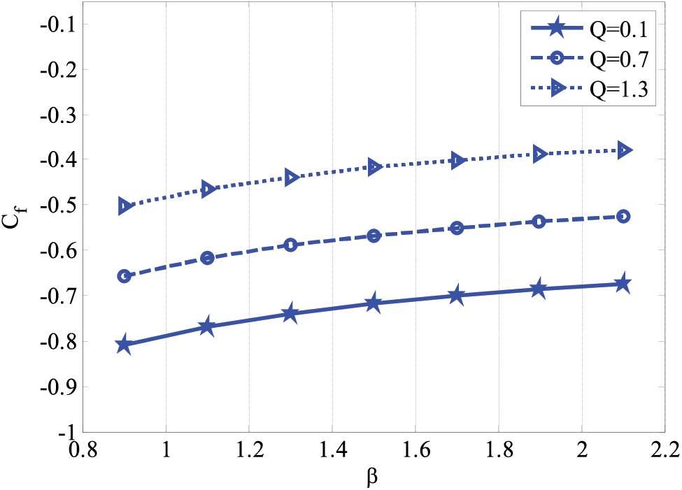
Figure 11: Effect of Newtonian fluid with rescaled viscosity parameter and modified Hartmann number on skin friction coefficient using

Figure 12: Effect of reaction rate parameter on local Nusselt number using

Figure 13: Effect of reaction rate parameter and Schmidt number on local Sherwood number using

Figure 14: Contour plot for the horizontal component of velocity using

Figure 15: Contour plot for the vertical component of velocity using

Figure 16: Contour plot for temperature profile using
Fig. 17 shows the relative error made by the proposed scheme for the classical derivative. The scheme solves the example studied in [46]. The solved example is a two-dimensional problem that has the exact solution. Fig. 17 can be used to validate the results.
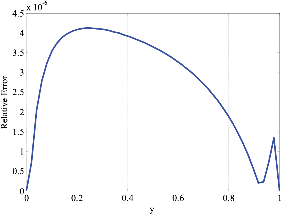
Figure 17: Relative error computed by the scheme for the classical case,
Table 1 shows the comparison of three schemes for finding the error and computational cost when these schemes are applied to 1st example considered in [47]. A scheme comparison is made for this example since the exact solution is available for this problem. The comparison shows that the proposed scheme provides smaller errors than the other two existing schemes. The first-order scheme is the forward Euler method, whereas the second-order scheme is just the second-order Runge-Kutta method. The proposed scheme produced better results but took more time to achieve them. So, the proposed scheme is more computationally expensive than the other two existing schemes. Also, it can be seen that the error is reduced by increasing the size of time levels or decreasing the size of the time step. The suggested scheme can be expanded in the following directions [48,49].

An innovative computer approach called the Fractal Runge-Kutta Method has been developed in this study. Its purpose is to address the challenging fractal time-dependent issues in fluid dynamics, namely the magnetohydrodynamic (MHD) Newtonian fluid with rescaled viscosity fluid flow on Riga plates. Several essential facts and insights have contributed significantly to the field due to the study. We confirm its robustness in dealing with the complexities of fractal dynamics by showing that the three-stage computing method, built with multiple time levels, is stable under Fourier series analysis for a scalar problem. The suggested method is further supported by a convergence analysis for the time-dependent fractal partial differential equations system, which gives a strong basis for its use in real-world situations. A dimensionless fractal model of incompressible, unstable, laminar Newtonian fluid with rescaled viscosity fluid flow over flat and oscillatory Riga plates successfully employs the computational scheme, demonstrating its adaptability. The numerical framework is further improved and more applicable to various fluid dynamic situations by discretizing the continuity equation using first-order back differences. A finite difference scheme has been constructed. The scheme was applied for fractal time-dependent partial differential equations of boundary layer flow over the flat and oscillatory sheets. The proposed scheme and backward differencing formulas have solved four dimensionless differential equations. Space discretization was done using second-order central difference formulas. The concluding points can be expressed as:
1. Skin friction coefficient has grown by enhancing the modified Hartmann number and Newtonian fluid with rescaled viscosity parameter.
2. Local Nusselt number declined by raising Eckert number and coefficient of temperature-dependent heat source term.
3. The local Sherwood number was increased by growing reaction rate parameter values and Schmidt number values.
Notable results include investigating how the skin friction and local Nusselt number are affected by the heat source’s temperature-dependent term coefficient. The findings show interesting patterns that show how fluid dynamics is affected by characteristics that depend on temperature. With this information, we can better comprehend how different factors interact in fractal fluid flow models.
In general, when dealing with time-dependent fluid dynamics problems, especially those involving fractal phenomena, the Fractal Runge-Kutta Method is an effective tool. This new and challenging field of study can build upon the analytical stability and convergence investigations conducted and practical applications to Newtonian fluid flow with rescaled viscosity fluid over Riga plates. With the growing knowledge of fractal dynamics, the computational technique proposed here could be helpful in many areas of fluid mechanics.
Integrating multi-physics phenomena, experimental validation or comparison with empirical data, practical applications in aerospace engineering, heat exchanger design, or chemical processing industries, and extension to complex geometries and boundary conditions could be the focus of future research. Another area of interest could be developing and applying advanced fractal techniques for time-dependent fractal MHD Casson fluid dynamics over moving Riga plates. We aim to include various viewpoints in the conclusion to lay out a thorough plan for future research efforts, encouraging creativity and progress in the area.
Acknowledgement: The authors wish to express their gratitude to Prince Sultan University for facilitating the publication of this article through the Theoretical and Applied Sciences Lab.
Funding Statement: The authors would like to acknowledge the support of Prince Sultan University in paying the article processing charges (APC) for this publication.
Author Contributions: Conceptualization, methodology, and analysis, writing—review and editing, Yasir Nawaz; funding acquisition, Kamaleldin Abodayeh; investigation, Yasir Nawaz; methodology, Muhammad Shoaib Arif; project administration, Kamaleldin Abodayeh; resources, Kamaleldin Abodayeh; supervision, Muhammad Shoaib Arif; visualization, Kamaleldin Abodayeh; writing—review and editing, Muhammad Shoaib Arif; proofreading and editing, Muhammad Shoaib Arif. All authors reviewed the results and approved the final version of the manuscript.
Availability of Data and Materials: The manuscript included all required data and implementing information.
Ethics Approval: Not applicable.
Conflicts of Interest: The authors declared no potential conflicts of interest concerning this article’s research, authorship, and publication.
References
1. Tani I. History of boundary layer theory. Annu Rev Fluid Mech. 1977;9(1):87–111. doi:10.1146/annurev.fl.09.010177.000511. [Google Scholar] [CrossRef]
2. Ishtiaq B, Nadeem S, Alzabut J, Alzabut C. Thermal analysis of magnetized Walter’s-B fluid with the application of Prabhakar fractional derivative over an exponentially moving inclined plate. Phys Fluids. 2023;35(12):102319. doi:10.1063/5.0179491. [Google Scholar] [CrossRef]
3. Kumar RSV, Dhananjaya PG, Kumar RN, Gowda RJP, Prasannakumara BC. Modeling and theoretical investigation on Casson nanofluid flow over a curved stretching surface with the influence of magnetic field and chemical reaction. Int J Comput Methods Eng Sci Mech. 2022;23(1):12–9. doi:10.1080/15502287.2021.1900451. [Google Scholar] [CrossRef]
4. Nadeem S, Ishtiaq B, Alzabut J, Eldin SM. Three parametric Prabhakar fractional derivative-based thermal analysis of Brinkman hybrid nanofluid flow over exponentially heated plate. Case Stud Therm Eng. 2023;47(10):103077. doi:10.1016/j.csite.2023.103077. [Google Scholar] [CrossRef]
5. Pantokratoras A, Magyari E. EMHD free-convection boundary-layer flow from a Riga-plate. J Eng Math. 2009;64(3):303–15. doi:10.1007/s10665-008-9259-6. [Google Scholar] [CrossRef]
6. Devi SPA, Devi SSU. Numerical investigation of hydromagnetic hybrid Cu-Al2O3/water nanofluid flow over a permeable stretching sheet with suction. Int J Non-linear Sci Numer Simul. 2016;17:249–57. doi:10.1515/ijnsns-2016-0037. [Google Scholar] [CrossRef]
7. Deka RK, Gupta AS, Takhar HS, Soundalgekar VM. Flow past an accelerated horizontal plate in a rotating fluid. Acta Mech. 1999;138:13–9. doi:10.1007/BF01179538. [Google Scholar] [CrossRef]
8. Mazumdar MK, Deka RK. MHD flow past an impulsively started infinite vertical plate in presence of thermal radiation. Rom J Phys. 2007;52(5–6):529–35. [Google Scholar]
9. Fatima N, Belhadj W, Nisar KS, Alaoui MK, Arain MB, Ijaz N. Heat and mass transmission in a boundary layer flow due to swimming of motile gyrotactic microorganisms with variable wall temperature over a flat plate. Case Stud Therm Eng. 2023;45:102953. doi:10.1016/j.csite.2023.102953. [Google Scholar] [CrossRef]
10. Mukhopadhyay S, Mondal IC, Chamkha AJ. Casson fluid flow and heat transfer past a symmetric wedge. Heat Transf Asian Res. 2013;42:665–75. doi:10.1002/htj.21065. [Google Scholar] [CrossRef]
11. Pantokratoras A. The Blasius and Sakiadis flow along a Riga-plate. Progr Comput Fluid Dyn Int J. 2011;11:329. doi:10.1504/PCFD.2011.042184. [Google Scholar] [CrossRef]
12. Gailitis A, Lielausis O. On the possibility of drag reduction of a flat plate in an electrolyte. Appl Magnetohydrodyn Trudy Inst Fisiky AN Latvia SSR. 1961;12:143. [Google Scholar]
13. Eswaramoorthi S, Alessa N, Sangeethavaanee M, Namgyel N. Numerical and analytical investigation for Darcy-Forchheimer flow of a Williamson fluid over a Riga plate with double stratification and Cattaneo-Christov dual flux. Adv Math Phys. 2021; 2021(1):1867824. doi:10.1155/2021/1867824. [Google Scholar] [CrossRef]
14. Reyaz R, Mohamad AQ, Jiann LY, Saqib M, Shafie S. Presence of Riga plate on MHD Caputo Casson fluid: an analytical study. J Adv Res Fluid Mech Therm Sci. 2022;93:86–99. doi:10.37934/arfmts.93.2.8699. [Google Scholar] [CrossRef]
15. Abbas MS, Shaheen A, Abbas N, Shatanawi W. Mathematical model of second-grade Casson fluid flow with Soret and Dufour impact over Riga sheet. Modern Phys Lett B. 2024;38(25):2450230. doi:10.1142/S0217984924502300. [Google Scholar] [CrossRef]
16. Zainal NA, Nazar R, Naganthran K, Pop I. Unsteady stagnation point flow past a permeable stretching/shrinking Riga plate in Al2O3-Cu/H2O hybrid nanofluid with thermal radiation. Int J Numer Methods Heat Fluid Flow. 2022;32:2640–58. doi:10.1108/HFF-08-2021-0569. [Google Scholar] [CrossRef]
17. Loganathan P, Deepa K. Computational exploration of Casson fluid flow over a Riga-plate with variable chemical reaction and linear stratification. Nonlinear Anal Model. 2020;25:443–60. doi:10.15388/namc.2020.25.16659. [Google Scholar] [CrossRef]
18. Kumar M, Mondal PK. Bejan’s flow visualization of buoyancy-driven flow of a hydromagnetic Casson fluid from an isothermal wavy surface. Phys Fluids. 2021;33(9):465. doi:10.1063/5.0060683. [Google Scholar] [CrossRef]
19. Bilal S, Asogwa KK, Alotaibi H, Malik M, Khan I. Analytical treatment of radiative Casson fluid over an isothermal inclined Riga surface with aspects of chemically reactive species. Alex Eng J. 2021;60(5):4243–53. doi:10.1016/j.aej.2021.03.015. [Google Scholar] [CrossRef]
20. Sun H, Zhang Y, Baleanu D, Chen W, Chen Y. A new collection of real world applications of fractional calculus in science and engineering. Commun Nonlinear Sci. 2018;64:213–31. doi:10.1016/j.cnsns.2018.04.019. [Google Scholar] [CrossRef]
21. Saad KM, Atangana A, Baleanu D. New fractional derivatives with non-singular kernel applied to the Burgers equation. Chaos. 2018;28(6):063109. doi:10.1063/1.5026284. [Google Scholar] [PubMed] [CrossRef]
22. Atangana A, Baleanu D. New fractional derivatives with nonlocal and non-singular kernel: theory and application to heat transfer model. Thermal Science. 2016;20(2):763–9. doi:10.2298/TSCI160111018A. [Google Scholar] [CrossRef]
23. Bas E, Ozarslan R. Real world applications of fractional models by Atangana-Baleanu fractional derivative. Chaos Solitons Fractals. 2018;116:121–5. doi:10.1016/j.chaos.2018.09.019. [Google Scholar] [CrossRef]
24. Tassaddiq A, Khan I, Nisar KS, Singh J. MHD flow of a generalized Casson fluid with Newtonian heating: a fractional model with Mittag-Leffler memory. Alex Eng J. 2020;59:3049–59. doi:10.1016/j.aej.2020.05.033. [Google Scholar] [CrossRef]
25. Shah NA, Ebaid A, Oreyeni T, Yook SJ. MHD and porous effects on free convection flow of viscous fluid between vertical parallel plates: advance thermal analysis. Waves Random Complex Media. 2023;1–13. doi:10.1080/17455030.2023.21867. [Google Scholar] [CrossRef]
26. Shah NA, Asogwa KK, Mahsud Y, Lee S, Kang S, Chung JD, et al. Effect of generalized thermal transport on MHD free convection flows of nanofluids: a generalized Atangana-Baleanu derivative model. Case Stud Therm Eng. 2022;40:102480. [Google Scholar]
27. Jan SAA, Ali F, Sheikh NA, Khan I, Saqib M, Gohar M. Engine oil based generalized Brinkman-type nano-liquid with molybdenum disulphide nanoparticles of spherical shape: atangana-Baleanu fractional model. Num Methods Partial Diff Equ. 2018;34(9):1472–88. [Google Scholar]
28. Saqib M, Khan I, Shafie S. Application of Atangana-Baleanu fractional derivative to MHD channel flow of CMC-based-CNT’s nanofluid through a porous medium. Chaos Solitons Fractals. 2018;116:79–85. [Google Scholar]
29. Khan M, Rasheed A. Scott-Blair model with unequal diffusivities of chemical species through a Forchheimer medium. J Mol Liq. 2021;341:117351. [Google Scholar]
30. Nawaz Y, Arif MS, Abodayeh K. An explicit-implicit numerical scheme for time fractional boundary layer flows. Int J Numer Methods Fluids. 2022;94(7):920–40. [Google Scholar]
31. Nawaz Y, Arif MS, Abodayeh K. A third-order two-stage numerical scheme for fractional Stokes problems: a comparative computational study. J Comput Non-linear Dyn. 2022;17(10):101004. [Google Scholar]
32. Choi SUS, Eastman JA. Enhancing thermal conductivity of fluids with nanoparticles. J Adv Res Fluid Mech Therm Sci. 2018;44(1):131–9. [Google Scholar]
33. Majewski P, Thierry B. Functionalized magnetite nanoparticles—synthesis, properties, and bio-applications. Crit Rev Solid State Mater Sci. 2007;32(3–4):203–15. doi:10.1080/10408430701776680. [Google Scholar] [CrossRef]
34. Hussanan A, Salleh MZ, Khan I. Microstructure and inertial characteristics of a magnetite ferrofluid over a stretching/shrinking sheet using effective thermal conductivity model. J Mol Liq. 2018;255(1):64–75. doi:10.1016/j.molliq.2018.01.138. [Google Scholar] [CrossRef]
35. Seth GS, Mandal PK. Gravity-driven convective flow of magnetite-water nanofluid and radiative heat transfer past an oscillating vertical plate in the presence of magnetic field. Latin Am Appl Res. 2018;48(1):7–13. doi:10.52292/j.laar.2018.250. [Google Scholar] [CrossRef]
36. Crane LJ. Flow past a stretching plate. Z Angew Math Phys ZAMP. 1970;21(4):645–7. doi:10.1007/BF01587695. [Google Scholar] [CrossRef]
37. Dandapat BS, Gupta AS. Flow and heat transfer in a viscoelastic fluid over a stretching sheet. Int J Nonlin Mech. 1989;24(3):215–9. doi:10.1016/0020-7462(89)90040-1. [Google Scholar] [CrossRef]
38. Andersson HI, Hansen OR, Holmedal B. Diffusion of a chemically reactive species from a stretching sheet. Int J Heat Mass Transf. 1994;37:659–64. [Google Scholar]
39. Nadeem S, Rehman A, Lee C, Lee J. Boundary layer flow of second grade fluid in a cylinder with heat transfer. Math Probl Eng. 2012;2012:13. [Google Scholar]
40. Majeed A, Zeeshan A, Alamri SZ, Ellahi R. Heat transfer analysis in ferromagnetic viscoelastic fluid flow over a stretching sheet with suction. Neural Comput Appl. 2018;30:1947–55. [Google Scholar]
41. Privalova VV, Prosviryakov EY. A new class of exact solutions of the Oberbeck-Boussinesq equations describing an incompressible fluid. Theor Found Chem Eng. 2022;56(3):331–8. [Google Scholar]
42. Baranovskii ES, Shishkina OY. Generalized boussinesq system with energy dissipation: existence of stationary solutions. Mathematics. 2024;12(5):756. [Google Scholar]
43. Prabhakar Reddy B, Matao PM, Sunzu JM. A finite difference study of radiative mixed convection MHD heat propagating Casson fluid past an accelerating porous plate including viscous dissipation and Joule heating effects. Heliyon. 2024;10(7):E28591. doi:10.1016/j.heliyon.2024.e28591. [Google Scholar] [PubMed] [CrossRef]
44. Fuzhang W, Akhtar S, Nadeem S, El-Shafay AS. Mathematical computations for the physiological flow of Casson fluid in a vertical elliptic duct with ciliated heated wavy walls. Waves Random Complex Media. 2022;1–14. doi:10.1080/17455030.2022.20729. [Google Scholar] [CrossRef]
45. Wang F, Ahmad S, Al Mdallal Q, Alammari M, Khan MN, Rehman A. Natural bio-convective flow of Maxwell nanofluid over an exponentially stretching surface with slip effect and convective boundary condition. Sci Rep. 2022;12(1):2220. [Google Scholar] [PubMed]
46. Dehghan M. Fourth-order techniques for identifying a control parameter in the parabolic equations. Int J Eng Sci. 2002;40(4):433–47. doi:10.1016/S0020-7225(01)00066-0. [Google Scholar] [CrossRef]
47. Li F, Wu Z, Ye C. A finite difference solution to a two-dimensional parabolic inverse problem. Appl Math Model. 2012;36(5):2303–13. doi:10.1016/j.apm.2011.08.025. [Google Scholar] [CrossRef]
48. Arif MS, Abodayeh K, Nawaz Y. The modified finite element method for heat and mass transfer of unsteady reacting flow with mixed convection. Front Phys. 2022;10:952787. doi:10.3389/fphy.2022.952787. [Google Scholar] [CrossRef]
49. Nawaz Y, Arif MS, Bibi M, Abbasi JN, Javed U, Nazeer A. A finite difference method and effective modification of gradient descent optimization algorithm for MHD fluid flow over a linearly stretching surface. Comput Mater Contin. 2020;62(2):657–77. doi:10.32604/cmc.2020.08584. [Google Scholar] [CrossRef]
Cite This Article
 Copyright © 2024 The Author(s). Published by Tech Science Press.
This work is licensed under a Creative Commons Attribution 4.0 International License , which permits unrestricted use, distribution, and reproduction in any medium, provided the original work is properly cited.
 Downloads
 Citation Tools