DeepBio: A Deep CNN and Bi-LSTM Learning for Person Identification Using Ear Biometrics

1  Introduction

In the dynamic realm of biometric identification, scholars and technology enthusiasts are perpetually exploring novel avenues to augment precision and efficacy. In the pursuit of establishing individual identity, biometrics of the ear has surfaced as a captivating area of study, utilizing the unique characteristics of the human ear [1]. The intricate and distinctive ears of humans can serve as a dependable biometric trait for detection purposes, despite often being overlooked. To perform human identification, the majority of biometric methods necessitate the participation of the corresponding individual to obtain their biometric characteristics. Exploring ear biometrics offers a helpful alternative during the COVID-19 pandemic. Conventional facial recognition systems encounter difficulties in accurately functioning due to the obstruction caused by masks, which cover a substantial part of the face. Due to this factor, facial recognition systems experience significant drawbacks, necessitating revisions in current systems [2]. Ear biometrics provides a dependable and unobtrusive approach, as ears are less likely to be concealed and display distinct features that remain consistent over time. Exploring and advancing research and development in this field has the potential to greatly improve biometric identification systems, guaranteeing strong and secure authentication even in situations where face characteristics are not completely visible [3]. Using fingerprint and palmprint recognition methods may not be appropriate in COVID-19. Iris recognition systems are expensive due to the specialized sensors required to extract iris features. Furthermore, it is noteworthy that the aforementioned biometric systems necessitate the individual’s cooperation to facilitate identification. A biometric system that is contactless and non-cooperative, such as ear biometrics, is currently in high demand [4].

The structure of the human ear remains stable from birth and exhibits individual uniqueness. The ear structure is depicted in Fig. 1. The ear comprises several morphological components, including the scapha, helix, Tagus, concha, antihelix, lobule, antitragus, and other anatomical structures. As the structure of the ear appears relatively uncomplicated, discernible differences among the ears are apparent even between identical twins. Consequently, the examination of auricular images to extract distinct and recognizable characteristics for individual identification and authentication is a current area of study and a developing intelligent biometric technology [5].

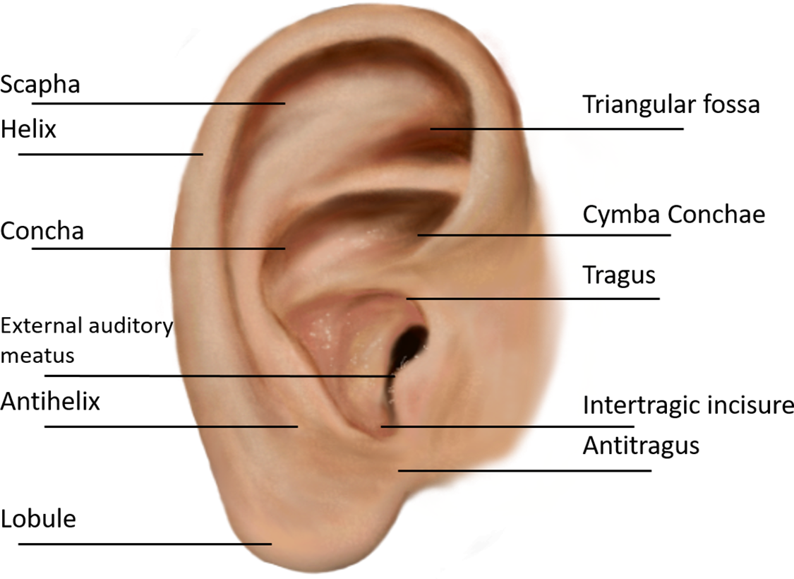
Figure 1: Anatomy of the ear: navigating the complexities of the human ear

Moreover, the method of acquiring auditory information through the human ear is both contactless and nonintrusive, thereby avoiding the need for cooperation from the individual being recognized. The utilization of ear biometric technology has the potential to function as a complementary component to other biometric modalities within automated recognition systems [6]. This can offer valuable identity indicators when alternative information sources are deemed untrustworthy or inaccessible. In surveillance, identifying individuals through facial recognition technology may encounter difficulties when dealing with profile faces. However, it is observed that the ear can provide valuable information regarding the identity of individuals captured in surveillance footage [7]. The utilization of ear images for automated human identification has garnered significant attention in academic research due to its potential commercial applications. Extracting features and using them in human identification using complex ear structures is tedious. The development and deployment of precise ear biometric systems face several challenges, including deficient image quality, ear shape, and orientation inconsistencies, and inadequate access to comprehensive ear image databases. Therefore, there is a need for computation techniques like Deep Learning (DL) to perform accurate identification of humans using ear biometrics [8]. By harnessing the unique and stable features of the human ear, coupled with the power of Machine Learning (ML) and DL models, researchers are paving the way for accurate, robust, and versatile biometric systems.

In this study, we introduced a framework called DeepBio, which integrates two DL methodologies: Convolutional Neural Network (CNN) and Bidirectional Long Short-Term Memory (Bi-LSTM), for human identification utilizing ear biometrics. Initially, data augmentation techniques such as flipping, translation, and Gaussian noise are employed to enhance performance and mitigate overfitting. This is followed by the hybrid of the CNN and Bi-LSTM models for feature extraction and human identification. We conduct experiments using five distinct datasets: IIT Delhi (IITD-I, IITD-II), annotated web images (AWE), mathematical analysis of images (AMI), and EARVN1. Finally, we evaluate the framework’s performance using four key metrics: recognition rate, sensitivity, precision, and F1-score.

1.1 Research Contributions

The following are the research contributions of the DeepBio:

•   Utilization of flipping, translation, and Gaussian noise augmentation techniques, aimed at mitigating overfitting.

•   Adoption of a hybrid approach combining CNN and Bi-LSTM for ear identification.

•   Incorporation of IITD-I, IITD-II, AWE, AMI, and EARVN1 datasets for training and validation.

•   Demonstration of the efficacy of DeepBio in human identification utilizing ear biometrics, as evidenced by the final results.

1.2 Critical Analysis

Ear biometrics play an important role in human identification, especially in cases where face recognition fails, as in the COVID-19 pandemic. The existing work employed various feature extraction [9], ML, and DL techniques for human identification. Most authors have worked on CNN for human identification. However, none of the existing work advanced DL algorithms, like LSTM, for identification. Moreover, they have yet to work on hybrid techniques for human identification. Hence, a hybrid CNN and Bi-LSTM model is developed using ear biometrics to identify humans.

The subsequent sections are given as follows: The review on the state-of-the-art techniques is given by Section 2. The background information and preliminary concepts are provided in Section 3. The detailed description of the DeepBio is described in Section 4, followed by the exposition of the results in Section 5. Ultimately, Section 6 outlines the conclusion drawn from the findings.

2  Literature Review

Various researchers have explored computational techniques for human identification. Zhang et al. [10] discussed few-shot learning approaches comprising model-agnostic meta-learning (MAML) algorithm, first-order model-agnostic meta-learning (FOMAML), and Reptile algorithm implemented on a CNN using the AMI dataset. Augmentation techniques such as flipping, cropping, rotation, and brightness adjustment were employed and integrated into the few-shot learning process. The conducted experiment demonstrated promising results with a recognition rate of 93.96%. Hassaballah et al. [11] proposed an algorithm termed averaged local binary patterns (ALBP) technique. Extensive tests were conducted on five ear datasets, achieving results of 96.94%, 96.34%, 73%, 38.76%, and 39% for each dataset, respectively. Sarangi et al. [12] presented a novel automated approach aimed at enhancing the ear images by leveraging the improved version of the Jaya metaheuristics. Empirical results suggest that the proposed image enhancement approach performs comparably to conventional methods.

Moving ahead, Sajadi et al. [13] presented a method for extracting distinctive features from the ear region using Contrast-limited Adaptive Histogram Equalization (CAHE) and Gabor-Zernike (GZ) operator. Subsequently, a Genetic Algorithm (GA) is applied to identify for classification. A more practical strategy is proposed by Korichi et al. [14] wherein they propose a technique named TR-ICANet combining Independent Component Analysis (ICA) and a Tied-Rank (TR) for ear print identification. Empirical investigations have been conducted and the evaluations showed that the TR-ICANet performed better than various existing techniques. Mehraj et al. [15] utilized a proactive data augmentation technique, InceptionV3 architecture, Principal Component Analysis (PCA), and Support Vector Machine (SVM) for human identification. The quadratic SVM model attained the highest results of 98.1% accuracy. Similarly, Omara et al. [16] developed a method by employing a deep CNN for feature extraction and applying a Mahalanobis distance metric for learning. The Mahalanobis distance was computed using the LogDet divergence metric learning technique. Finally, K-Nearest Neighbors (KNN) was utilized for ear recognition purposes. The study’s results indicate that the developed approach outperforms current ear recognition techniques.

Additionally, Khaldi et al. [17] proposed deep convolutional generative adversarial networks (DCGAN) and CNN models. The experiment was conducted and the performed experiments demonstrated favorable results compared to existing techniques. A more practical strategy is proposed by Ahila Priyadharshini et al. [18] introduced a deep CNN consisting of six layers for ear recognition. The effectiveness of this approach is assessed on two distinct datasets: the IITD-II and the AMI dataset. Based on the outcomes, it was concluded that the strategy that was provided functioned exceptionally well, obtaining high recognition rates. Similarly, Hasan et al. [19] provided the Automated Ear Pinna Identification (AEPI) method for human identification. The conducted experiment shows the effectiveness of the proposed approach.

Furthermore, Xu et al. [20] introduced an ELERNet, based on MobileNet V2 architecture for human ear images. A comparison was made between the ELERNet model and the MobileNet V2 model, and the results demonstrate that the suggested work is effective. Through the utilization of a single-layer unsupervised lightweight network, Aiadi et al. [21] introduced a unique approach for ear print identification known as Magnitude and Direction with Feature Maps Neural Network (MDFNet). Ear alignment was initially accomplished through the utilization of CNN and PCA. Subsequently, a dual-layer approach was employed, comprising convolution with learned filters and computation of a gradient image. The proposed method outperforms compared to various contemporary techniques, showcasing notable resilience to occlusion. Mehta et al. [22] presented a methodology that involves the stacking of three CNN models that have been pre-trained for identification purposes. The experiment was carried out showing an accuracy of 98.74%. Singh et al. [23] presented a deep learning model named CNN for gender classification using the EARVN1 dataset. The proposed method showed less computational complexity and performed well with an accuracy of 93%. Similarly, Alshazly et al. [24] presented ResNet, DenseNet, MobileNet, and Inception for the identification of humans using AMI dataset. The combination of CNN and transfer learning methods performed well showing a recognition rate of 96%. In addition, the visualization approach known as Gradient-weighted Class Activation Mapping (Grad-CAM) was used to clarify the decision-making processes of the models. This technique revealed that the models tend to rely on auxiliary features such as hair, cheek, or neck, whenever they are present. Utilizing Grad-CAM not only improves comprehension of the decision-making mechanisms within the CNNs but also illuminates possible areas for enhancing the proposed ear recognition systems. Hossain et al. [25] employed transfer learning on pre-trained models, namely YOLO (V3, V5) and MobileNet-SSD (V1, V2), to train and assess the effectiveness of these models in identifying individuals using ear biometrics. The models underwent training using the Pascal VOC, COCO, and Open Image datasets, and subsequently underwent retraining using the EarVN1.0 dataset. According to the research findings, the YOLOV5 model demonstrated superior performance compared to YOLOV3, MobileNet-SSDV1, and MobileNet-SSDV2 in terms of accuracy and efficiency when it comes to identifying individuals based on ear biometrics.

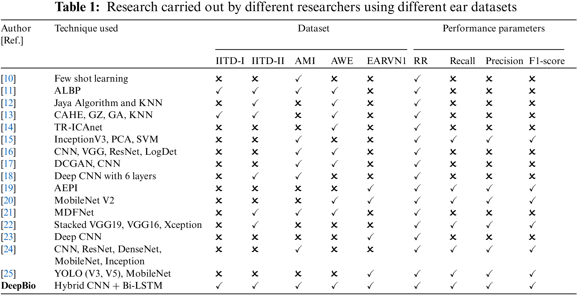
The existing literature predominantly relies on fundamental CNN models and traditional ML algorithms. Surprisingly, advanced DL algorithms like LSTM have been largely overlooked. The utilization of LSTM networks in ear biometrics shows great potential because of their capacity to capture temporal relationships and process sequential data [26]. LSTMs, due to their structure consisting of memory cells and gates, are highly efficient at collecting extended relationships and temporal patterns that are essential for biometric applications. Within the field of ear biometrics, LSTM models are utilized to analyze sequences of ear images. By taking into account the temporal information, LSTMs can detect subtle patterns and traits that traditional approaches may overlook. This results in enhanced accuracy and resilience to changes in position, lighting conditions, and occlusion. In addition, they possess the ability to effectively manage occlusions and noise through the examination of image sequences. Furthermore, they may be seamlessly incorporated with other biometric modalities to develop recognition systems that are more complete in nature. Although there may not be many studies specifically focused on using LSTM for ear biometrics, research in adjacent fields like face and gait recognition shows that LSTMs are useful in capturing temporal dynamics and enhancing performance [27]. Consequently, there’s a gap in leveraging these powerful techniques for tasks such as human identification using ear biometrics. To address this void, we introduce the DeepBio framework, which amalgamates CNN and Bi-LSTM architectures. The research conducted by different researchers is detailed in Table 1.

3  Background Information and Preliminary Concepts

3.1 Data Augmentation

Data augmentation is used in ML to artificially expand the amount and diversity of a training dataset by modifying or transforming existing data. The augmented data is formed by modifying the original samples slightly, resulting in new comparable examples but not identical to the originals. It is an effective strategy for boosting model performance, decreasing overfitting, expanding dataset size, and making models more resilient and generalizable. It gives the model the ability to learn from a broader set of events and variations, resulting in improved performance on previously unseen data [28]. Different data augmentation techniques comprise rotation, scaling, translation, flipping, noise injection, blurring, occlusion, contrast and brightness adjustment, and elastic deformations. Rotation is rotating the ear images by various angles to imitate the varied stances, which helps learn the data in various orientations. Rescaling is zooming in or out of ear images which helps the model learn to adapt to differences in the size and distance of the ears from the camera. Moving ahead is the translation that helps the model manage differences in ear location by shifting the ear pictures horizontally or vertically within the frame to represent varying placements of the ears. The act of horizontally mirroring ear images, commonly referred to as flipping, has the potential to generate supplementary training samples and facilitate the acquisition of invariant features by the model, which are not influenced by left-right orientation. The technique of noise injection involves the introduction of stochastic noise into auditory images, which can enhance the model’s resilience to fluctuations in ambient illumination and sensor interference. The blurring technique, which involves the application of blur filters to ear images, can facilitate the learning process of the model by reducing its sensitivity to minor details and enhancing its focus on broader features. The occlusion technique involves the superimposition of patches or objects onto specific regions of ear images. This approach facilitates the acquisition of knowledge by the model, enabling it to identify ears even in situations where partial occlusion is present. Contrast and brightness adjustment is the process of adjusting contrast and brightness levels in ear images can potentially improve the model’s capacity to accommodate varying lighting conditions. Elastic deformation is the application of elastic deformations to ear images that can introduce local shape variations, thereby enhancing the model’s resilience to deformations in ear appearance [29].

In the current study, three data augmentation techniques, including flipping, translation, and noise injection, are applied that help the model to learn with different variations, to improve the model performance and reduce overfitting effectively.

3.2 Convolution Neural Network (CNN)

CNNs are a specific category of advanced machine learning models designed to effectively analyze and manipulate data like images, audio, and videos for classification, segmentation, and detection. Inspired by the structural organization of the visual cortex in living beings, CNNs comprise layers of neurons that respond to specific localized regions of the input data, enabling them to effectively extract features and patterns from visual information [30]. CNN consists of convolutional, pooling, and fully connected layers which are delineated in the following section and shown in Fig. 2:

•   Input: The input layer of the network is responsible for receiving the initial data, which can be in the form of an image or a video frame. The dimensions of the input layer indicate the magnitude and quantity of channels present in the input data, such as the Red Green Blue (RGB) channels in an image.

•   Convolutional Layer: The convolutional layers are responsible for executing the primary operation within a CNN, which is commonly referred to as convolution. Every stratum comprises several filters, also known as kernels, that are matrices of small size. The filters undergo a systematic sliding process over the input image and execute element-wise multiplications and summations, resulting in the production of a feature map. Obtaining relevant characteristics from the data that is being input is the primary goal of the convolutional algorithm. The Eq. (1) is used to extract the feature map. Let’s consider a single channel (grayscale) input image and a single filter for simplicity. For each image of size Hidin×Weiin and a kernel of size Ker×Ker, the feature map (output) is computed by the following Eq. (1):

feature_map[row, col]=∑m=0Ker−1⁡∑n=0Ker−1⁡input_image[row+m,col+n]×filter[m,n](1)

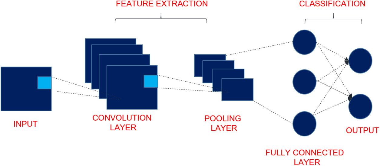
Figure 2: Structure of CNN

In this equation, feature_map[row,col] represents the computed result at position (row, col). input_image[row+m,col+n] corresponds to the pixel values in the local responsive field of the input image covered by the filter, and filter [m,n] denotes the learnable filter coefficients.

•   Activation Function: Commonly, an element-wise application of a nonlinear activation function is performed on the feature map after each convolutional layer. The incorporation of nonlinearity in the network facilitates the acquisition of intricate patterns and relationships within the data. Section 3.4 describes several activation functions, including Rectified Linear Unit (ReLU), Scaled Exponential Linear Unit (SELU), Exponential Linear Units (ELU), sigmoid, and hyperbolic tangent (Tanh), and softmax.

•   Pooling Layers: The pooling layers perform downsampling on the feature maps derived from the convolutional layers, thereby decreasing their spatial dimensionality while preserving the salient data. The prevalent technique for pooling is the max pooling operation, which entails selecting the highest value within each designated pooling region. The implementation of pooling techniques contributes to enhancing the network’s resilience to minor translations while simultaneously decreasing the computational demands.

•   Fully Connected Layers: Layers that are fully connected, sometimes referred to as dense layers, are those that form connections between each neuron of the layer that came before it and the neurons of the layer that is currently involved. These layers are designed to be similar to those that are found in conventional artificial neural networks. It is common practice to reduce the output of the final pooling layer to a 1D vector, which is subsequently sent across several fully connected layers. This process is repeated until the output is uniformly distributed. In classification jobs, these layers are frequently utilized because they are capable of performing sophisticated nonlinear operations.

•   Output: The outcomes of the neural network are given by the output layer, which is the final level of the network and is responsible for creating predictions. Depending on the nature of the problem that is being solved, the activation function that is used for the final layer is determined.

Apart from the primary layers, CNN may incorporate supplementary elements such as normalization layers (e.g., Batch Normalization) to enhance training stability and regularization techniques (e.g., Dropout) to avert overfitting.

3.3 Bidirectional Long Short Term Memory (Bi-LSTM)

The Bi-LSTM model comprises two LSTM layers, with the first LSTM layer processing the input sequence in the forward direction and the second LSTM layer processing it in the backward way [31]. LSTM was developed to successfully describe long-term relationships in sequential data and to solve issues such as vanishing gradient conditions. This is accomplished by incorporating memory cells, gates, and a variety of mechanisms for information flow into the system. The Bi-LSTM design enhances the model’s ability to record both previous and succeeding contexts in a sequence, making it beneficial for jobs that necessitate the evaluation of both past and future variables to provide accurate outputs [32]. The detailed working of Bi-LSTM is given in Fig. 3, and the components are described below:

•   Input: The input sequence refers to a type of sequential data structure that is subject to processing by the Bi-LSTM model.

•   Forward LSTM: The input sequence is sequentially processed from start to finish in the forward LSTM layer, enabling the identification and recording of dependencies and patterns within the sequence. This method incorporates several different components, such as concatenation, input gate, forget gate, output gate, and candidate cell state. To generate an augmented feature vector, concatenation is used by combining the prior hidden state (hid(t−1)) with the current input (xt). Furthermore, the input gate decides how much new information should be added to the cell state, and the forget gate decides how much of the old state should be retained. The output gate is responsible for controlling the amount of the cell state that should be revealed as the output. To update the current cell state (cellt), it is necessary to take into account the input gate, the forget gate, and the candidate cell state. On the other hand, the current hidden state (hidt) can be retrieved by applying the output gate to the updated cell state. Through the use of mathematics, the Eq. (2) is used to convey both the current cell state and the current concealed state.

concat=[hidt−1,xt]Input gate (it)=σ(Weii⋅concat+biasi)Forget gate (ft)=σ(Weif⋅concat+biasf)Output gate (ot)=σ(Weio⋅concat+biaso)Candidate cell state (gt)=tanh⁡(Weig⋅concat+biasg)State of Current cell (cellt)=ft⊙cellt−1+it⊙gtCurrent hidden state (hidt)=ot⊙tanh⁡(cellt)(2)

    where σ represents a sigmoid function, ⊙ denotes element-wise multiplication, Wei and biasf represent weights and bias value.

•   Backward LSTM: The LSTM layer that operates in a reverse direction, commencing from the end of the input sequence and concluding at the beginning, is referred to as the backward LSTM layer. The input sequence’s dependencies and patterns are captured in a retrograde manner. Similarly, like forward LSTM, backward LSTM’s new cell state and hidden state can be calculated and given by Eq. (3) as follows:

Current cell state(cellt)=ft⊙cellt+1+it⊙gtCompute the current hidden state(hidt)=ot⊙tanh⁡(cellt)(3)

    where ft is forgot gate, it is input gate, and gt denotes candidate cell state.

•   Concat Layer: Upon conducting bidirectional processing of the input sequence, the resulting outputs from the forward and backward LSTM layers are subsequently merged through concatenation. This process of concatenation involves the integration of data obtained from both historical and prospective contexts.

•   Fully Connected Layer: Fully connected layers, also referred to as dense layers, are commonly incorporated after the Bi-LSTM layers to perform additional processing on the concatenated outputs. The aforementioned strata possess the ability to acquire intricate representations and execute classification or regression tasks contingent upon the extracted characteristics.

•   Output Layer: It is the final layer which maps the processed features to the desired output format, depending on the task. For example, the output layer may use a softmax activation function in a classification task to produce class probabilities.

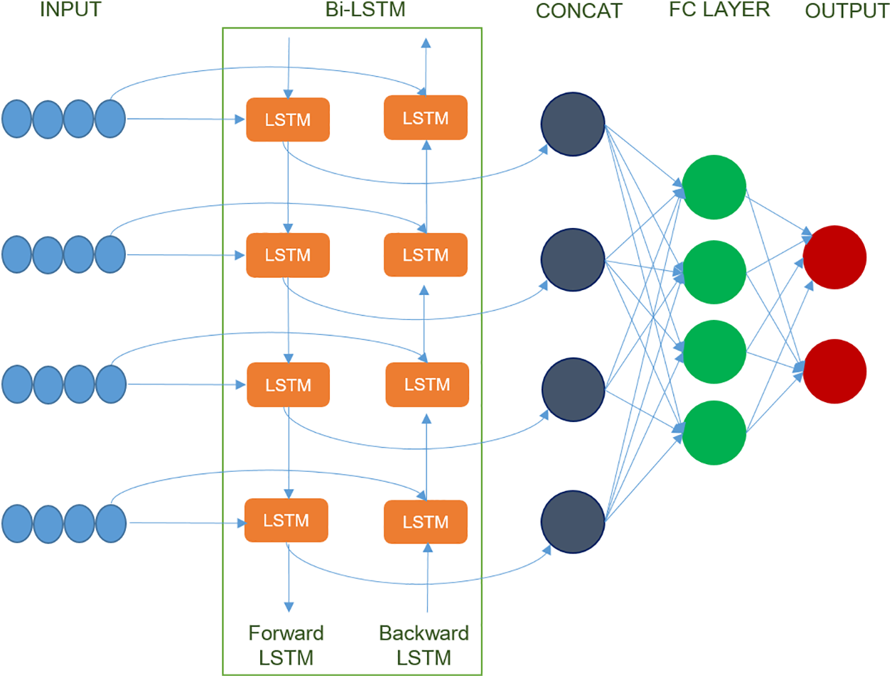
Figure 3: Working of Bi-LSTM

In this study, the output layer employs a softmax function, whereas the fully connected layer makes use of a ReLU activation function.

3.4 Activation Functions

An activation function is a mathematical operation that is applied to the output of neural network layers or neurons to bring non-linearity into the network [33]. They improve the expressiveness of the network and make it easier to learn complex patterns. There are many other activation functions available, such as the ReLU, ELU, SELU, Tanh, sigmoid, and softmax functions. RELU effectively and simply mitigates the impact of disappearing gradients. The fun(x) is changed to 0 for a negative value of x and it is changed to x when the value of x is either positive or 0 or both. There is no limit to the range of ReLU, which is [0,∞]. On the other hand, ELU and SELU both have a decreasing gradient for negative values. ELU makes use of a logarithmic curve, but SELU makes use of a scaled logarithmic curve. The sigmoid activation function having values ranging from 0 to 1 is used for making probability predictions. The hyperbolic tangent activation function, also known as tanh, is the bipolar counterpart of the sigmoid function. Its range extends from minus one to plus one. Tanh can effectively map negative inputs to substantially negative outputs while translating zero inputs to outputs that are close to zero. When it comes to multiclass classification tasks, the softmax function is a popular choice because of its more generalized variation. The mathematical formulations of all the activation functions are shown in Table 2. A further illustration of the graphical representations of these activation functions can be seen in Fig. 4. In CNN and Bi-LSTM, these functions are utilized at the fully linked layer of the network. Additionally, because the ear biometric human identification is a problem that involves multiple classes of categorization, the softmax function is utilized at the output layer.

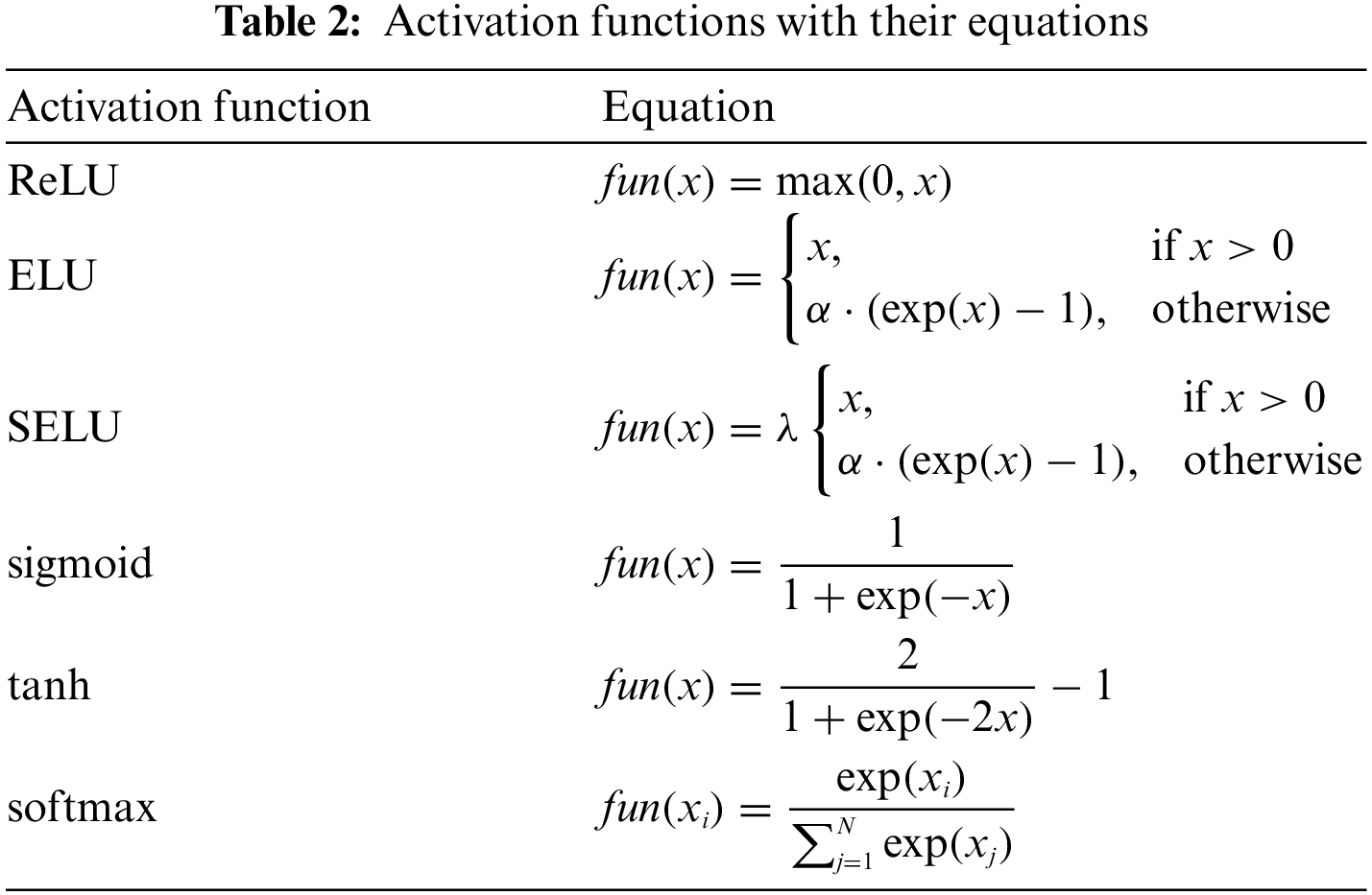
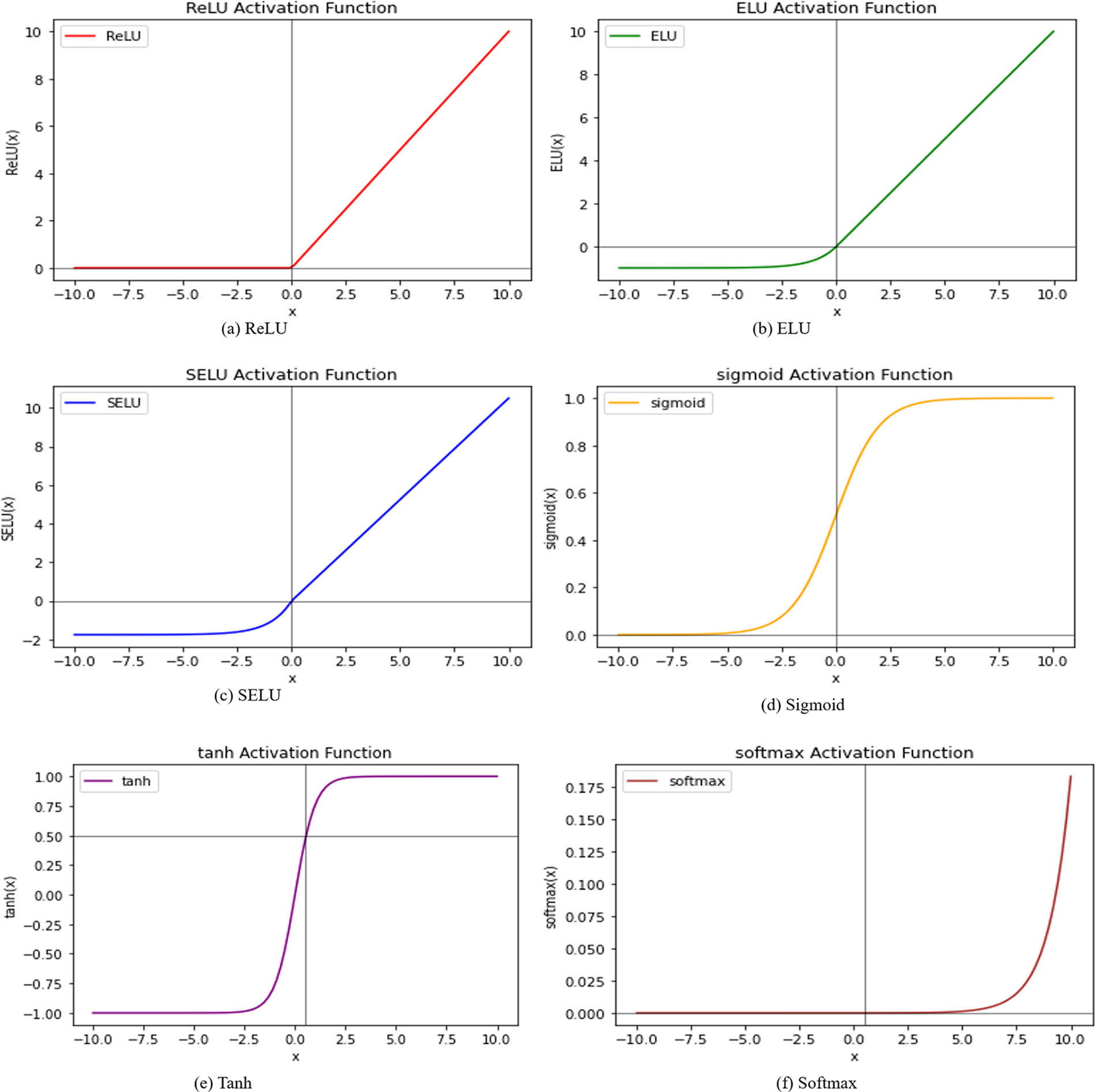
Figure 4: Curves for activation functions

4  Proposed Framework: DeepBio

In the present research, the DeepBio framework based on hybrid CNN + Bi-LSTM is proposed. First, image augmentation is done to prevent overfitting, followed by human identification using a hybrid of CNN and Bi-LSTM DL models. Five datasets, including IITD-I, IITD-II, AWE, AMI, and EARV1, are used to train and evaluate the model. Recognition rate, recall, F1-score, and precision are the four metrics used to measure performance. The workflow of DeepBio is given in Fig. 5 and is described below.

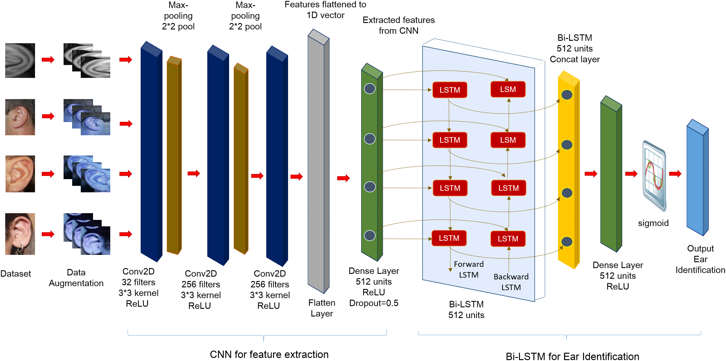
Figure 5: Workflow of DeepBio

4.1 Dataset

In our study, we utilize five datasets for human identification: IITD-I, IITD-II, AMI, AWE, and EARVN1. Using various datasets is a comprehensive method to assess a model’s performance in different scenarios. By utilizing a variety of datasets, we can evaluate the model’s capacity to apply its knowledge to various contexts, hence improving its resilience and dependability [34]. Sample images from each dataset are depicted in Fig. 6. Here’s a brief overview of each dataset.

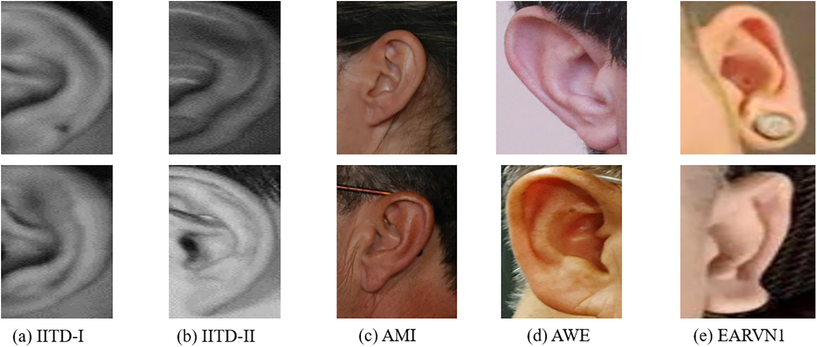
Figure 6: Samples of datasets

4.1.1 IIT Delhi (IITD)

Two datasets make up the IIT Delhi ear imaging database. These datasets are called IITD-I and IITD-II, and they each contain 125 and 221 participants, respectively [35]. The imaging process is non-invasive, conducted indoors using a simple setup, ensuring subjects are not physically manipulated during image acquisition. The age range of individuals in the database spans from 14 to 58 years old. Our study exclusively utilizes IITD-I and IITD-II datasets for experimentation. Cropped ear images, sized 50 × 180, are employed, with a total of 493 and 793 samples in both IITD-I and IITD-II, respectively.

4.1.2 Mathematical Analysis of Images (AMI)

A total of seven hundred ear images were taken from one hundred different people ranging in age from 19 to 65 years old for the AMI ear dataset [36]. There are a total of seven photographs provided for each subject, with six of those images devoted to the right ear and one image devoted to the left ear. Several different perspectives, including forward, left, right, up, and down, are utilized to obtain pictures of the right ear. A different focal length was used to catch the subject’s right ear in the sixth shot, which also features a zoomed-in perspective of the subject’s right ear. The subject is shown facing forward in the seventh picture, which represents the left ear. All of the images that are included in the collection have a resolution of 492 pixels squared.

4.1.3 Annotated Web Ears (AWE)

The AWE dataset was curated to encompass a wide variety of contexts by sourcing images from the internet. A diverse sample of 100 participants, spanning various ages, genders, and ethnicities, was selected. Each participant contributed ten closely cropped images [37]. There are a total of one thousand photos included in the AWE dataset, each of which has a different size.

4.1.4 EARVN1

The dataset known as EarVN1.0 was produced with the help of 164 people of Asian ethnicity as the sample population. This enormous database is comprised of 28,412 color pictures, including 98 male and 66 female subjects. It is considered to be one of the largest ear databases that are accessible to the scholarly community [38]. The fact that this dataset contains photos from both ears of each individual, which were taken in an unrestricted setting, is what differentiates it from other studies that have been conducted in the past. Following the extraction of ear pictures from facial shots, the images are cropped to accommodate major differences in location, scale, and illumination.

4.2 Data Augmentation

Data augmentation artificially expands the amount and diversity of a training dataset by modifying or transforming existing data. The complete description of the data augmentation and its types is given in Section 3.1. The current study applies flipping, translation, and gaussian noise. At first, the images from each dataset comprising IITD, AMI, AWE, and EARVN1 are cropped to a size of 50 × 180. This is done because all images are of different sizes, which makes it difficult for CNN to process the different size images. Then, the images are converted to RGB channels because RGB facilitates the precise depiction of diverse colors and their fusions. The IITD dataset is composed of images in the GRAY channel. Even after conversion to RGB, the images retain their original GRAY channel composition. The reason for this is that the conversion process cannot introduce color information that is absent in the original grayscale image. Once the cropping and coloring are done, the images are flipped, which creates a mirror image of the original image. Then the translation of 20% is done on the flipped images. It means the image is shifted along the x-axis (horizontal) and y-axis (vertical) by 20%. Once the images are translated, then a Gaussian noise of standard deviation (0.2) is added. The noise is added to the translated image to create a noisy version of the image. Incorporating Gaussian noise induces stochastic fluctuations in the pixel intensities, emulating actual noise or disturbances in the data. The implementation of this technique aids in mitigating overfitting and enhances the model’s robustness to noise present in the test dataset. Fig. 7 shows all datasets’ images before and after augmentation.

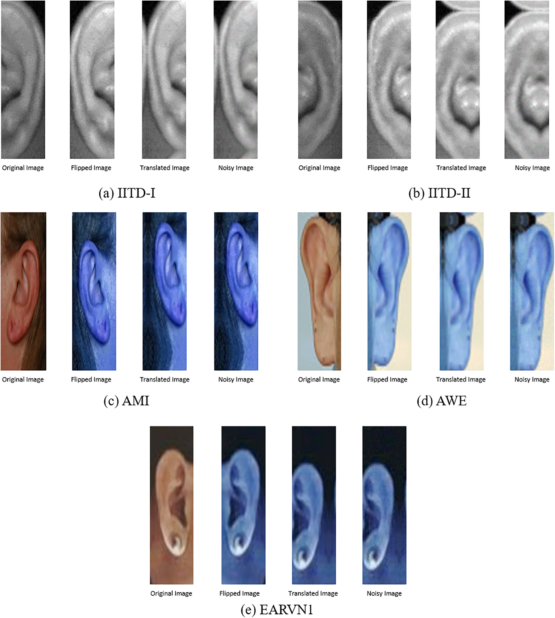
Figure 7: Samples before and after data augmentation

4.3 Hybrid CNN + Bi-LSTM

The current study employs a hybrid approach combining CNN and Bi-LSTM architectures for human identification. Initially, CNN is utilized to extract features from each dataset, serving as input for the subsequent Bi-LSTM model. The CNN structure is composed of three layers: the first layer uses 32 filters, the second layer is a 2 × 2 Max-pooling layer, the third layer is another layer with 256 filters and subsequent Max-pooling, and the final layer is a layer with 256 filters. A technique known as Max-pooling layers is utilized to reduce the spatial dimensions of the feature maps. In the following step, the characteristics are transformed into a one-dimensional vector. Furthermore, to further refine the features, a fully connected layer consisting of 512 units is applied, which is then supplemented by a dropout rate of 0.5 to prevent overfitting. ReLU activation function and a kernel size of 3 × 3 are employed throughout the experiment. Detailed explanations of the CNN and Bi-LSTM models’ operations are provided in Sections 3.2 and 3.3, respectively. The complete summary of CNN is given in Fig. 8 below:

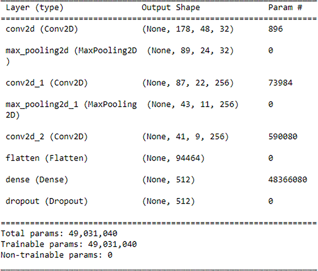
Figure 8: Summary of CNN

As depicted in Fig. 8, it can be observed that the initial Convolutional layer comprises 896 parameters, resulting in an output shape of (None, 178, 48, 32). Subsequently, a Max-pooling layer is implemented without any parameters, thereby decreasing the spatial dimensions by 50%, culminating in an output shape of (None, 89, 24, 32). Afterward, a Convolutional layer is employed, which comprises 73,984 parameters and yields an output shape of (None, 87, 22, 256). This is succeeded by a Max-pooling layer that does not involve any parameters, leading to an output shape of (None, 43, 11, 256). Then Convolutional layer with 590,080 parameters is used, resulting in an output shape of (None, 41, 9, 256). Subsequently, the Flatten layer transforms the tensor into a 1D vector of 94,464 units in length. This is succeeded by a Dense layer encompassing 48,366,080 parameters, resulting in an output configuration of (None, 512). Then a dropout layer is used, which randomly omits 50% of the input units during the training process. The aggregate count of trainable parameters within a CNN is 49,031,040, encompassing the summation of parameters across all layers.

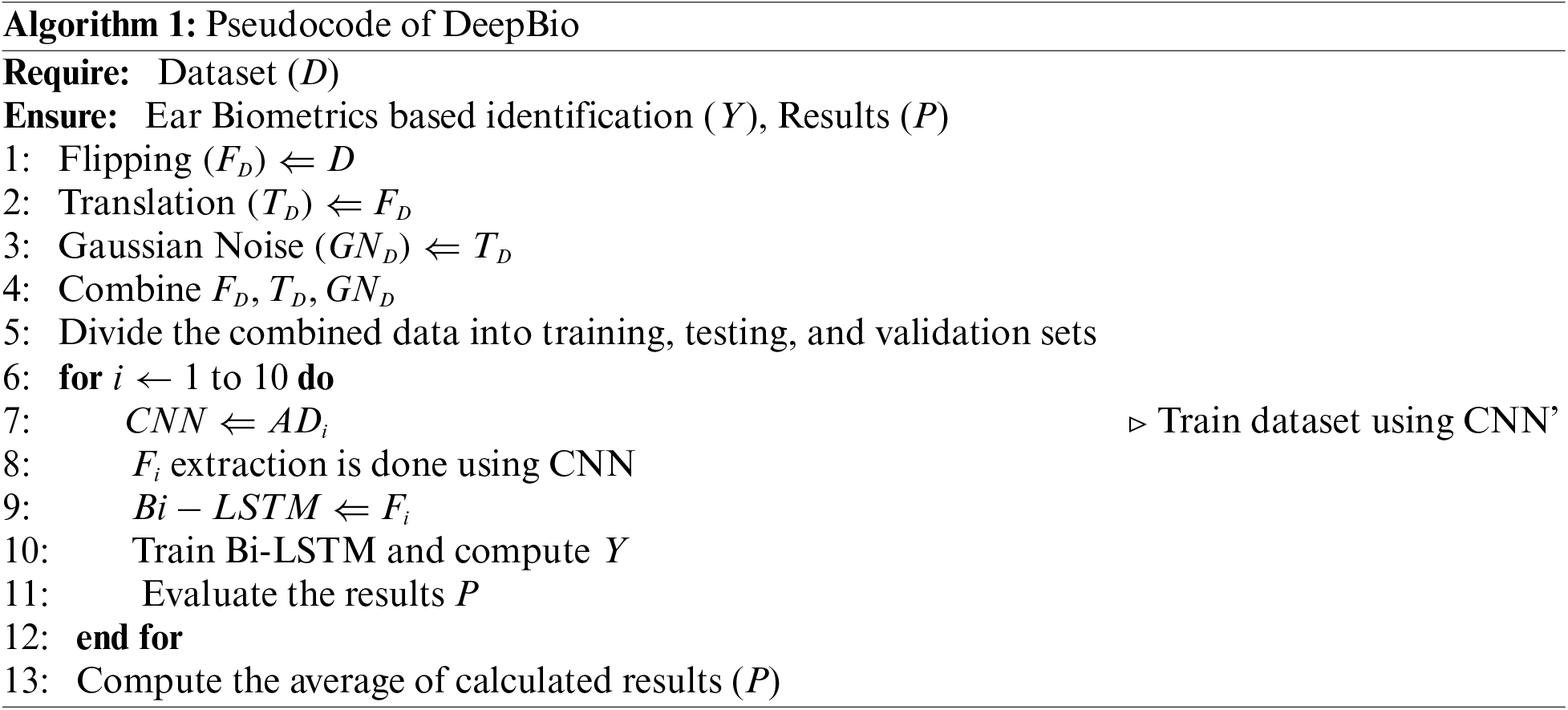
Following the completion of the feature extraction process, the recovered features are then input into a Bi-LSTM network for training and, more importantly, for use in human identification. In this study, a Bi-LSTM with 512 units is employed on the extracted features. Subsequently, another Bi-LSTM with 512 units is invoked to merge the outputs from both forward and backward LSTM units. Through the utilization of the ReLU, the output that has been combined is subsequently transmitted to a dense layer that is composed of 512 units. The output is then generated by employing the softmax activation function, which is used because the research is addressing a topic that involves the classification of many classes. A learning rate of 0.0001 is utilized by the Bi-LSTM in conjunction with the Adam optimizer for training. The summary of Bi-LSTM is shown in Fig. 9 below: The utilization of a Bi-LSTM layer with 4,198,400 parameters is illustrated in Fig. 9, resulting in an output shape of (None, 1, 1024). Subsequently, a Bi-LSTM layer with a parameter count of 6,295,552 is invoked, resulting in an output shape of (None, 1024). Subsequently, a dense layer comprising 524,800 parameters is employed, resulting in an output shape of (None, 512). Subsequently, a dense layer comprising 51,300 parameters is invoked as the ultimate layer, resulting in an output configuration of (None, 100). The aggregate count of trainable parameters within the model is 11,070,052, encompassing the summation of parameters across all layers. These summaries are for the AMI dataset. Similar summaries can be generated for the rest of the datasets. Algorithm 1 showcased the algorithm of the proposed DeepBio.

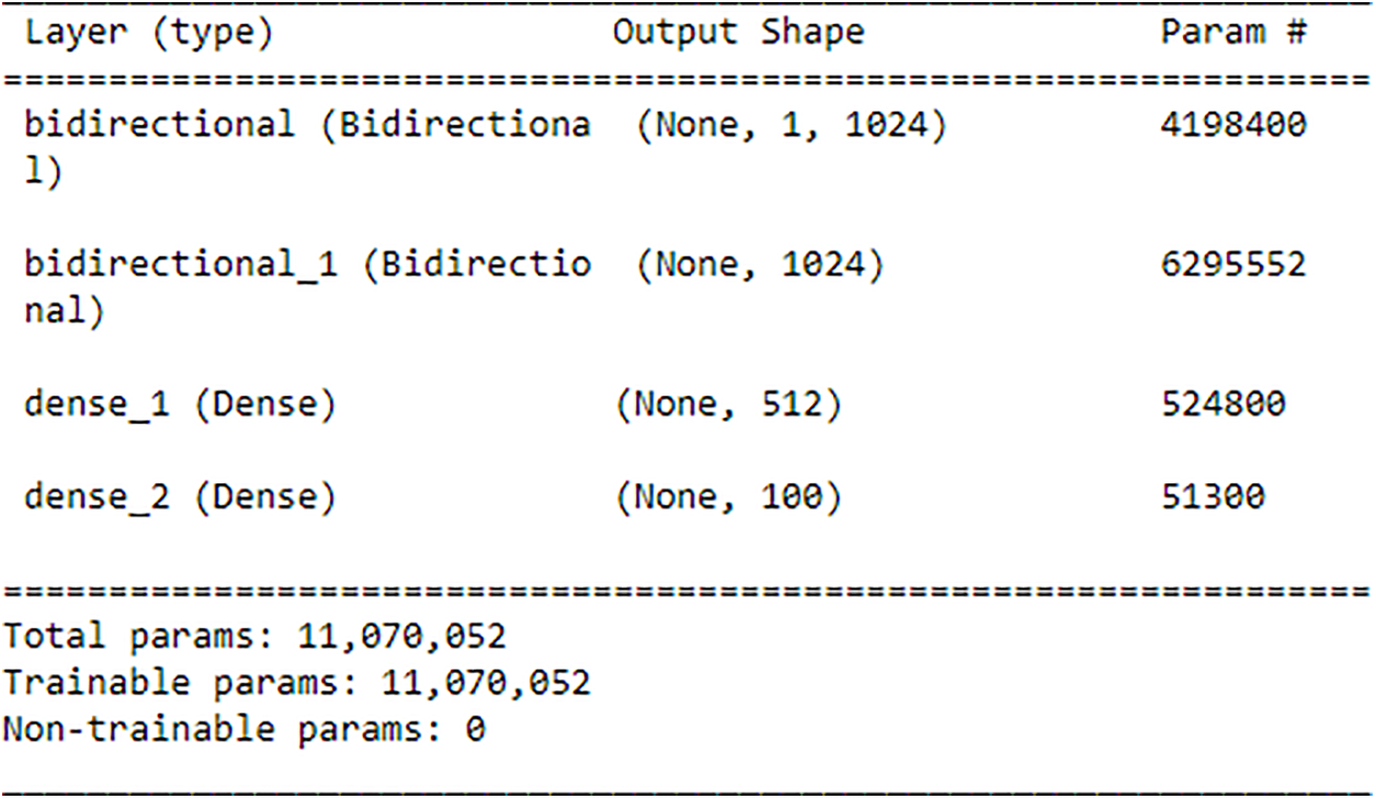
Figure 9: Summary of Bi-LSTM

5  Experimental Setup and Results

The current study introduces the DeepBio framework, which integrates CNN and Bi-LSTM models for human identification through ear biometrics. The datasets are split into two parts: one that is used for training and contains 80% of the data, while the other part is used for testing. A minimum hardware configuration of an i5 CPU and 8 GB of RAM is necessary for implementation. Python 3.9.0 serves as the primary programming language for development. The implementation relies on several libraries including cv2, os, numpy, Keras, Sequential, Conv2D, Flatten, MaxPooling2D, Dense, Bidirectional, Dropout, Adam, l2, keras.regularizers, and matplotlib. These libraries facilitate various tasks such as data handling, image processing, model building, optimization, and visualization. Four parameters comprising recognition rate, recall, precision, and F1-score are utilized to calculate the performance of the proposed DeepBio.

5.1 Results

Initially, original images undergo data augmentation techniques including flipping, translation, and the addition of Gaussian noise to diversify the dataset for varied perspectives. Subsequently, the dataset is split into an 80:20 ratio for training and testing, respectively. It is then fed into a hybrid model combining CNN and Bi-LSTM architectures. The experiment is repeated ten times, and performance metrics such as recognition rate, recall, precision, and F1-score are computed by averaging results across runs. The evaluation is conducted on multiple datasets, namely IITD-I, IITD-II, AMI, AWE, and EARVN1. The proposed DeepBio model demonstrates superior performance with recognition rates of 97.97%, 99.37%, 98.57%, 94.5%, and 96.87% for the respective datasets. Precision, recall, and F1-score are also calculated and displayed in Table 3.

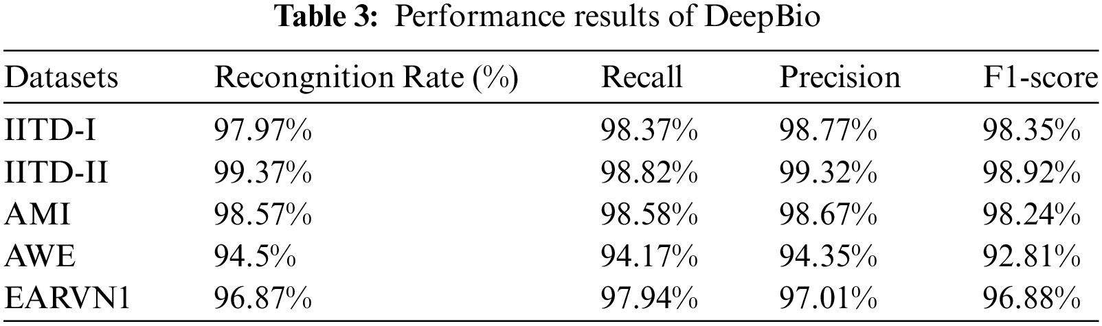
Furthermore, bar plots illustrating the computed parameters are presented in Fig. 10. The graphs show that DeepBio performed efficiently on the IITD-II dataset, with recall, precision, and F1-score of 98.82%, 99.32%, and 98.92%, respectively. The bar graphs show that DeepBio performed quite well on the IITD-II dataset.

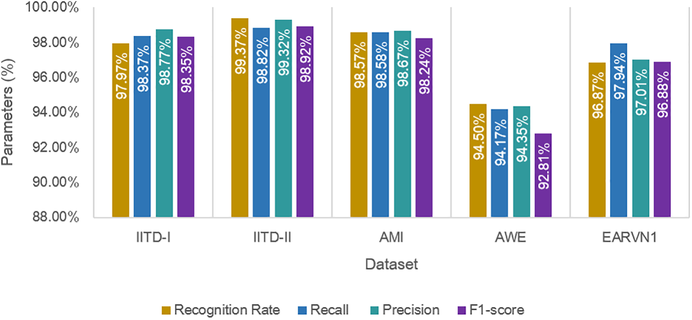
Figure 10: Performance results of DeepBio on all datasets

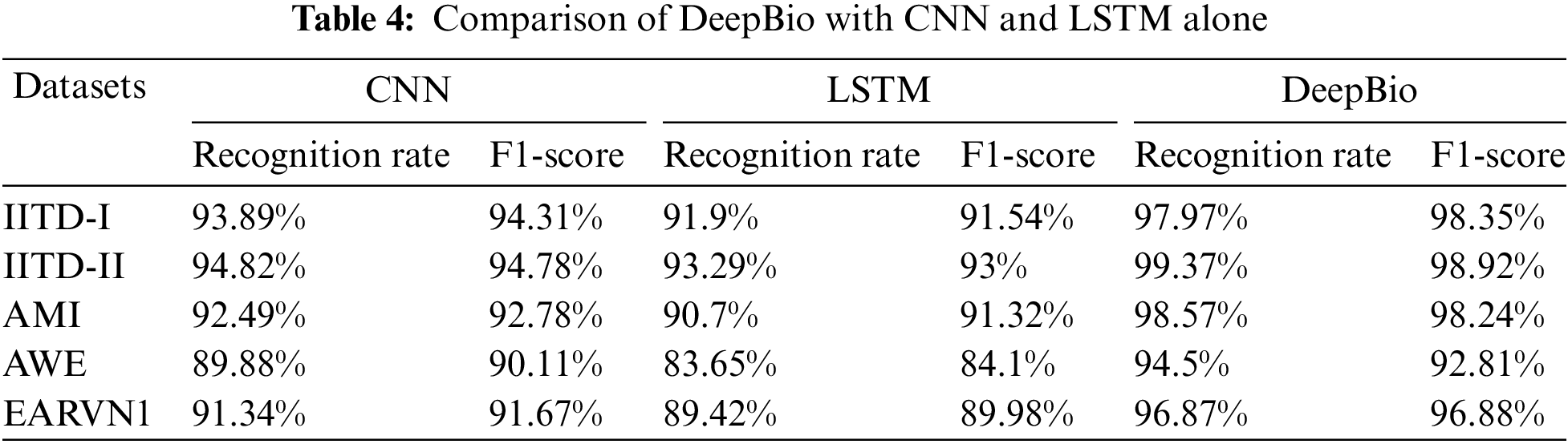
Additionally, the proposed DeepBio has been compared with CNN and LSTM alone. The recognition rate and F1-score for CNN and LSTM have been computed and shown in Table 4. The findings showed that the proposed DeepBio outperformed showing an improvement of 4.08%, 4.55%, 6.08%, 4.62%, and 5.53% in terms of recognition rate when compared with CNN. Similarly, DeepBio improves the result by 6.07%, 6.08%, 7.87%, 10.85%, and 7.45% in terms of recognition rate when compared with LSTM.

The training loss vs. validation loss and training accuracy vs. validation accuracy plots are also computed and displayed in Figs. 11 and 12. The CNN + Bi-LSTM runs for 50 epochs, and the Adam optimizer is used. The cross-entropy loss and accuracy value are computed for each epoch and plotted using the matplotlib library. The curves in Figs. 11 and 12 show that DeepBio performed effectively for each type. As the EARVN1 dataset size is large, it shows fluctuations in training and loss but performs well as the epochs increase.

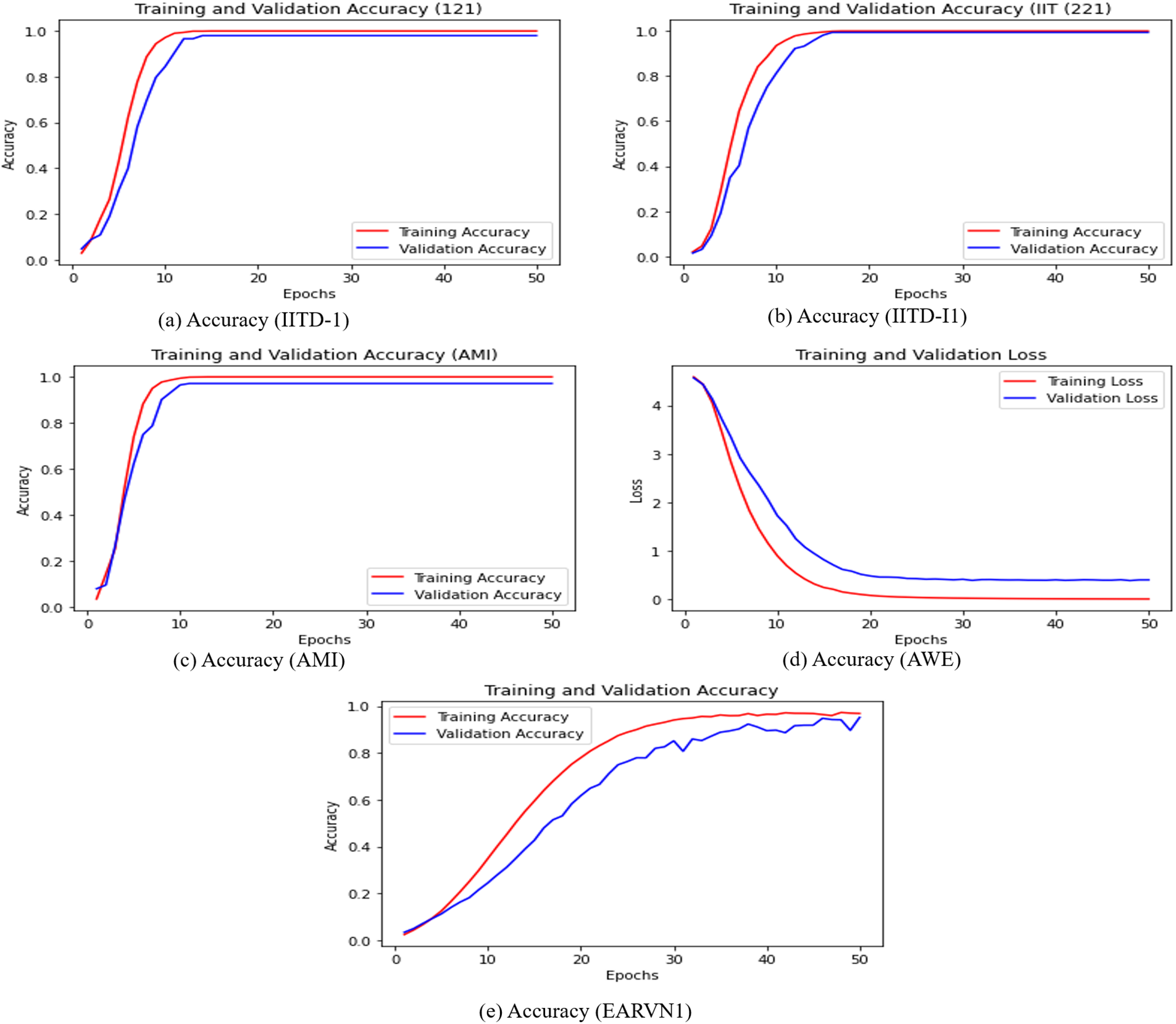
Figure 11: Training and validation accuracies

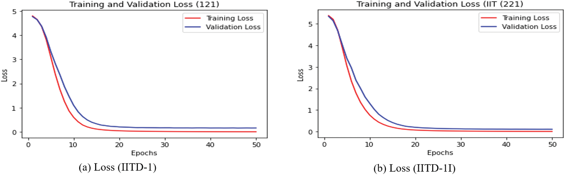
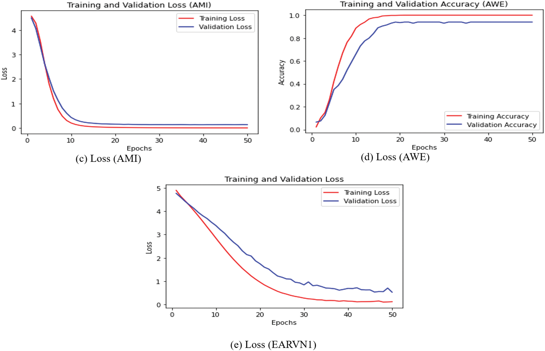
Figure 12: Training and validation loss

Additionally, along with precision, recall, and F1-score, cumulative curve (CMC) have been generated for each dataset and shown in Fig. 13. The CMC curve showed that the proposed DeepBio performed well with Rank-1 recognition rates of 97.97%, 99.37%, 98.57%, 94.5%, and 96.87% for IITD-I, IITD-II, AMI, AWE, and EARVN1 datasets, respectively.

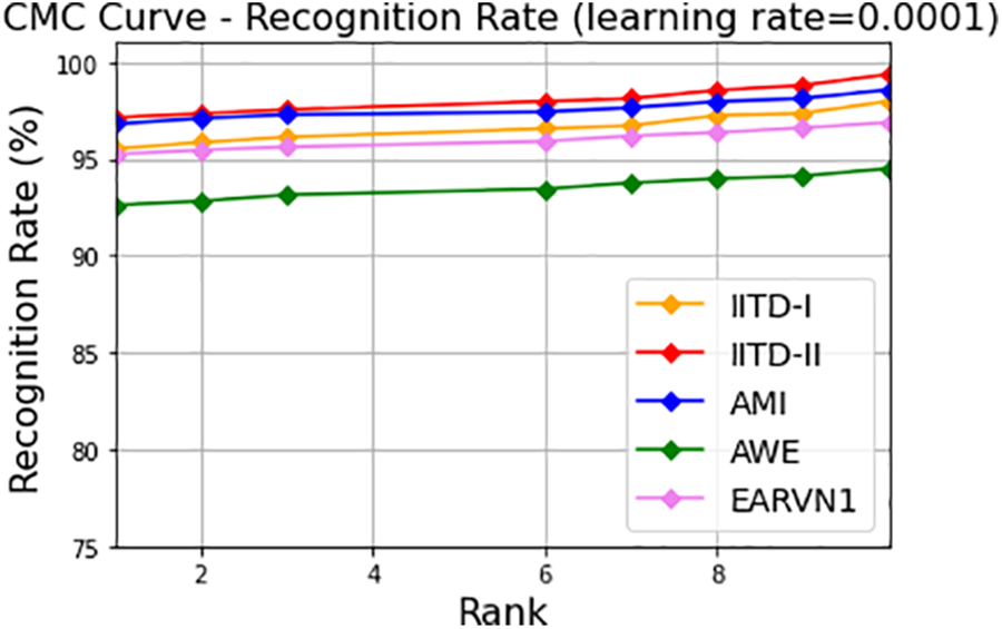
Figure 13: CMC curves showing Rank-1 recognition rates for IITD-I, IITD-II, AMI, AWE, and EARVN1

Furthermore, to test the performance of DeepBio in different uncontrolled environments, the results are computed on the dataset before augmentation, stage 1 augmentation, i.e., after flipping, and Gaussian noise, and stage 2 augmentation, i.e., after flipping, translation, and Gaussian noise effect, and it is found that the DeepBio performed well in stage 2 augmentation on IITD-II, AMI, AWE, and EARVN1 dataset. It shows an improvement of 2.51%, 4.28%, 2.5%, and 4.75% for IITD-II, AMI, AWE, and EARVN1 datasets, respectively, when compared with stage 1 augmentation. On the other side, for the IITD-I dataset, the stage 1 augmentation performed well with a recognition rate of 98.68% and show an improvement of 0.7% when compared to stage 2 augmentation. The reason why stage 1 augmentation performed better in IITD-I dataset is that, during stage 1, the augmentations employed are flipping and Gaussian noise. These augmentations potentially introduced advantageous variations that the model could acquire knowledge from, while not substantially modifying the fundamental characteristics of the images. These enhancements have the potential to improve the model’s resilience by instructing it to identify objects in various orientations and with minor pixel alterations. Stage 2, on the other hand, involved the processes of flipping, Gaussian noise, and translation. Although the flipping and Gaussian noise are preserved, the inclusion of translation may have caused distortions that shifted important features away from the central area of focus. This could potentially hinder the model’s ability to properly learn from these images. This might have resulted in an increase in irrelevant data and a decrease in valuable data, which would have had a detrimental impact on the model’s performance. The results of DeepBio on before augmentation and after stage 1 and stage 2 augmentation are shown in Table 5 below:

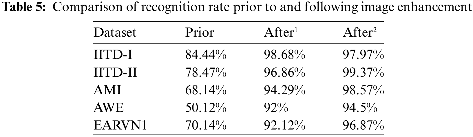
Moreover, the bar plots are plotted for before and after stage 1 and stage 2 augmentation and are shown in Fig. 14. It is visible from the plots that the DeepBio performed well and showed an improvement of 14.24%, 20.9%, 30.43%, 44.38%, and 26.73% for IITD-I, IITD-II, AMI, AWE, and EARVN1, respectively, when compared to before augmentation techniques. Furthermore, various activation functions like ReLU, SELU, ELU, and tanh are used to evaluate DeepBio’s performance. In both the convolutional and fully linked layers, these activation functions are employed. As a multi-class problem, the softmax function is used at the output layer for each activation function. The results are shown in Table 6. Further, the line plots are plotted as depicted in Fig. 15. The trends in the line plot show that the DeepBio outperforms on ReLU activation function, with Tanh as the second-best performer on all datasets.

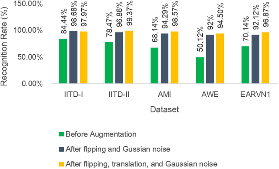
Figure 14: Recognition rate of DeepBio for before and after image augmentation

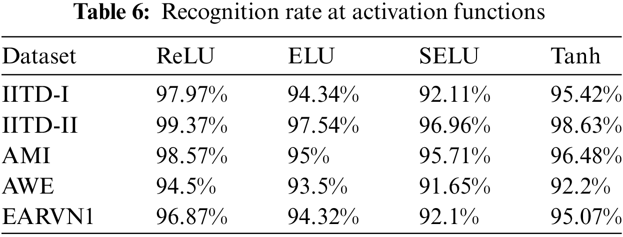
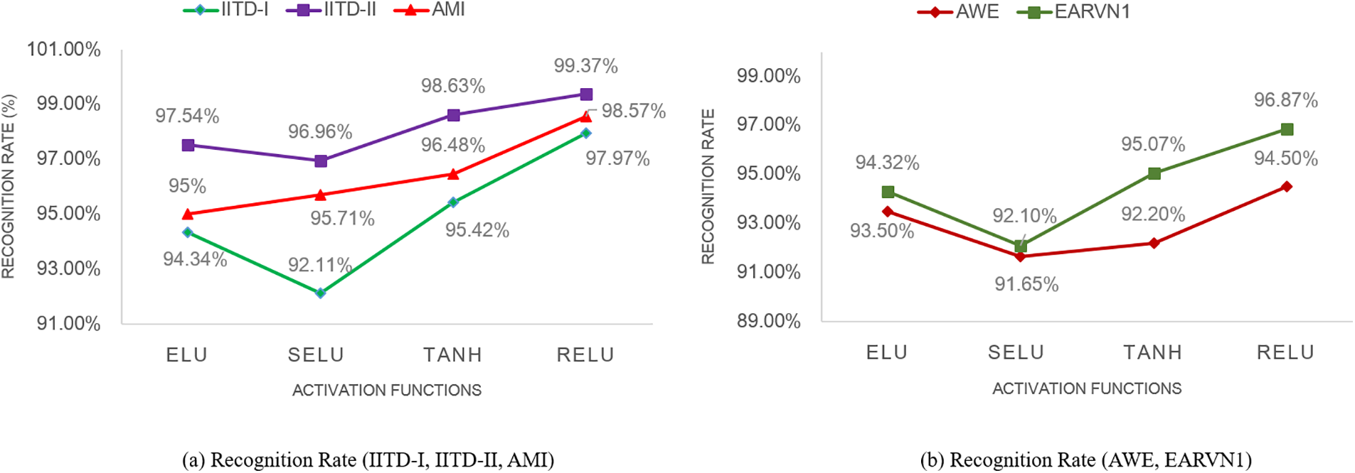
Figure 15: Recognition rate of DeepBio on different activation functions

Continuing, DeepBio is benchmarked against various state-of-the-art methods, as detailed in Table 7. With improvements of 0.41%, 0.47%, 12%, and 9.75% on the IITD-II, AMI, AWE, and EARVN1 datasets, respectively, DeepBio outperforms current methods.

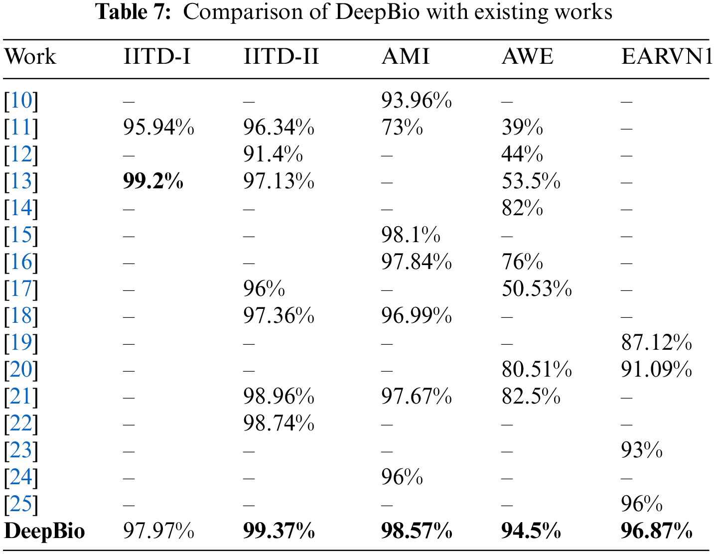
Additionally, the line plots are plotted to compare DeepBio with existing works and are shown in Fig. 16. The plot trend shows that the DeepBio performed efficiently on IITD-II, AMI, AWE, and EARVN1 datasets. DeepBio does not perform well in the IITD-I dataset compared to Sajadi et al. [13]. Only in this case, it lacks, on the rest of the datasets, it is performing effectively and achieving remarkable performance.

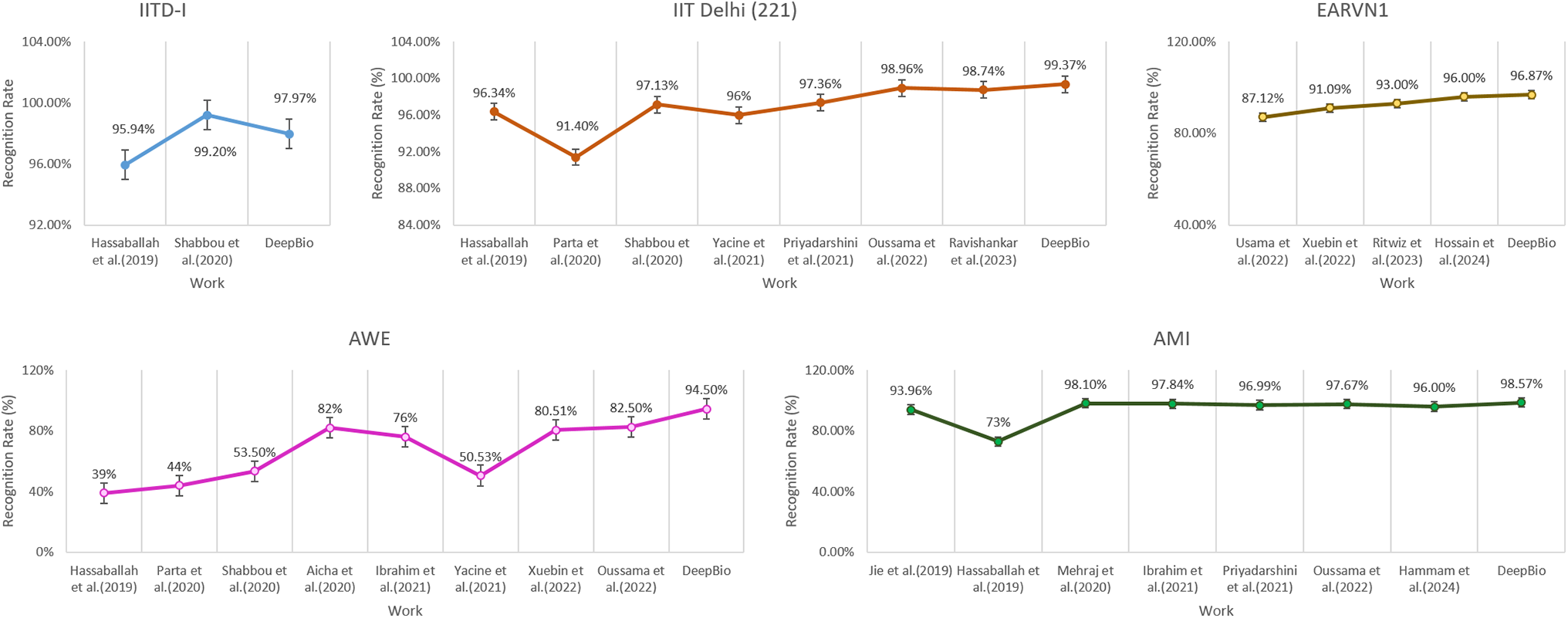
Figure 16: Comparison of DeepBio with existing works on all datasets

5.2 Discussions

The exceptional efficacy of the DeepBio model, which combines CNN and Bi-LSTM networks, can be ascribed to various factors, such as its hybrid structure, efficient data augmentation methods, and thorough evaluation metrics. CNNs are renowned for their capacity to autonomously and flexibly acquire spatial hierarchies of information from input images, a critical aspect of tasks such as image recognition. CNNs offer a strong basis for extracting features by collecting basic elements like edges and textures in the early layers and more intricate structures in the later layers. Conversely, Bi-LSTM networks improve this ability by analyzing data in both the forward and backward directions, capturing temporal relationships and contextual information. The bidirectional processing is especially advantageous in sequence modeling tasks, where comprehending the order and context of input data is crucial. DeepBio utilizes a combination of CNNs to extract spatial features and Bi-LSTMs to model sequences. This combination allows DeepBio to have a thorough grasp of both spatial and contextual data, resulting in enhanced performance metrics across various datasets. Data augmentation is crucial for improving the resilience and ability to generalize of DeepBio. Methods such as flipping, translation, and the incorporation of Gaussian noise introduce diversity into the training dataset, mimicking various viewpoints and environmental circumstances. Diversification is employed to mitigate overfitting, so ensuring that the model acquires the ability to recognize generic patterns that may be applied to new data, rather than merely memorizing the data it was trained on. The experimental findings demonstrate substantial enhancements in recognition rates following the implementation of data augmentation, particularly in stage 2 augmentation, which involves the integration of flipping, translating, and Gaussian noise. For example, the accuracy of identifying images in the IITD-II dataset increased from 78.47% before augmentation to 99.37% after stage 2 augmentation, demonstrating the efficiency of these strategies in enhancing the training process and improving the performance of the model. Moreover, DeepBio achieves a recognition rate of 99.37% for the IITD-II dataset, which is much higher than CNN’s 94.82% and LSTM’s 93.29%. This demonstrates the model’s improved capacity to reliably identify humans. Furthermore, DeepBio has an accuracy rate of 99.32%, recall rate of 98.82%, and an F1-score of 98.92% when applied to the IITD-II dataset. This performance surpasses that of both CNN and LSTM models, suggesting that DeepBio not only accurately detects real positive results but also minimizes the occurrence of false positive and false negative results. In addition, when compared to other advanced techniques, DeepBio has higher performance, with recognition rate improvements of up to 12% for datasets such as AMI and AWE. The comparisons emphasize the strong and effective performance of DeepBio in many situations and datasets, demonstrating its capacity to adapt and its superior design. The utilization of CNN and Bi-LSTM in DeepBio, in conjunction with the wide implementation of data augmentation techniques, guarantees that the model is trained on a varied and all-encompassing dataset, resulting in notable enhancements in performance. The extensive evaluation criteria and comparison with cutting-edge approaches further confirm its superiority, establishing DeepBio as a powerful model in the field of picture identification and classification.

6  Conclusion and Future Scope

The research on ear image identification holds significant importance in the biometric domain, especially amidst the COVID-19 pandemic where facial recognition systems face challenges due to widespread mask usage. Introducing ear biometrics can serve as an additional component to enhance automated human recognition systems. In this study, a DeepBio framework leveraging two deep learning models for ear biometric-based human identification is proposed. Five distinct datasets (IITD-I, IITD-II, AMI, AWI, and EARVN1) are utilized, undergoing data augmentation techniques such as flipping, translation, and Gaussian noise to enhance model performance and mitigate overfitting. A fusion of CNN and Bi-LSTM is employed for feature extraction and identification. DeepBio demonstrates promising performance with recognition rates of 97.97%, 99.37%, 98.57%, 94.5%, and 96.87% on the aforementioned datasets. Additionally, comparative analysis against established techniques shows improvements of 0.41%, 0.47%, 12%, and 9.75% on the IITD-II, AMI, AWE, and EARVN1 datasets, respectively. While DeepBio’s performance is satisfactory, further optimization of model parameters remains a potential avenue for future research. Nevertheless, the datasets employed (IITD-I, IITD-II, AMI, AWE, and EARVN1) may not fully encompass the range of variations encountered in real-life situations. Therefore, the proposed DeepBio will be enhanced by integrating a wider variety of datasets. Additionally, 10-fold cross-validation can be employed to enhance the performance of the proposed DeepBio. This strategy seeks to enhance the resilience, adaptability, generalizability, and comprehensiveness of our biometric identification systems.

Acknowledgement: None.

Funding Statement: The authors received no specific funding for this study.

Author Contributions: Anshul Mahajan implemented the work and wrote the manuscript; Sunil K. Singla reviewed the manuscript. All authors reviewed the results and approved the final version of the manuscript.

Availability of Data and Materials: The data will be made available on request.

Ethics Approval: Not applicable.

Conflicts of Interest: The authors declare that they have no conflicts of interest to report regarding the present study.

References

1. Jain AK, Nandakumar K, Ross A. 50 years of biometric research: accomplishments, challenges, and opportunities. Pattern Recognit Lett. 2016;79:80–105. doi:10.1016/j.patrec.2015.12.013. [Google Scholar] [CrossRef]

2. Talahua JS, Buele J, Calvopiña P, Varela-Aldás J. Facial recognition system for people with and without face mask in times of the COVID-19 pandemic. Sustainability. 2021;13(12):6900. doi:10.3390/su13126900. [Google Scholar] [CrossRef]

3. Zhang J, Liu Z, Luo X. Unraveling juxtaposed effects of biometric characteristics on user security behaviors: a controversial information technology perspective. Decis Support Syst. 2024 Aug 1;183:114267. doi:10.1016/j.dss.2024.114267. [Google Scholar] [CrossRef]

4. Kumar A, Singh SK. Recent advances in biometric recognition for newborns. In: The Biometric Computing. Chapman and Hall/CRC. 2019. p. 235–51. doi:10.1201/9781351013437-12. [Google Scholar] [CrossRef]

5. Emeršič Ž, Štruc V, Peer P. Ear recognition: more than a survey. Neurocomputing. 2017;255:26–39. doi:10.1016/j.neucom.2016.08.139. [Google Scholar] [CrossRef]

6. Sarangi PP, Nayak DR, Panda M, Majhi B. A feature-level fusion based improved multimodal biometric recognition system using ear and profile face. J Ambient Intell Humaniz Comput. 2022 Apr;13(4):1867–98. doi:10.1007/s12652-021-02952-0. [Google Scholar] [CrossRef]

7. Qin Z, Zhao P, Zhuang T, Deng F, Ding Y, Chen D. A survey of identity recognition via data fusion and feature learning. Inf Fusion. 2023;91:694–712. doi:10.1016/j.inffus.2022.10.032. [Google Scholar] [CrossRef]

8. Minaee S, Abdolrashidi A, Su H, Bennamoun M, Zhang D. Biometrics recognition using deep learning: a survey. Artif Intell Rev. 2023 Aug;56(8):8647–95. doi:10.1007/s10462-022-10237-x. [Google Scholar] [CrossRef]

9. Dhillon A, Singh A, Bhalla VK. A systematic review on biomarker identification for cancer diagnosis and prognosis in multi-omics: from computational needs to machine learning and deep learning. Arch Comput Methods Eng. 2023;30(2):917–49. doi:10.1007/s11831-022-09821-9. [Google Scholar] [CrossRef]

10. Zhang J, Yu W, Yang X, Deng F. Few-shot learning for ear recognition. In: Proceedings of the 2019 International Conference on Image, Video and Signal Processing, Shanghai, China; 2019; p. 50–4. doi:10.1145/3317640.3317646. [Google Scholar] [CrossRef]

11. Hassaballah M, Alshazly HA, Ali AA. Ear recognition using local binary patterns: a comparative experimental study. Expert Syst Appl. 2019;118:182–200. doi:10.1016/j.eswa.2018.10.007. [Google Scholar] [CrossRef]

12. Sarangi PP, Mishra BSP, Dehuri S, Cho SB. An evaluation of ear biometric system based on enhanced Jaya algorithm and SURF descriptors. Evol Intell. 2020;13(3):443–61. doi:10.1007/s12065-019-00311-9. [Google Scholar] [CrossRef]

13. Sajadi S, Fathi A. Genetic algorithm based local and global spectral features extraction for ear recognition. Expert Syst Appl. 2020;159(3):113639. doi:10.1016/j.eswa.2020.113639. [Google Scholar] [CrossRef]

14. Korichi A, Slatnia S, Aiadi O. TR-ICANet: a fast unsupervised deep-learning-based scheme for unconstrained ear recognition. Arab J Sci Eng. 2022;47(8):9887–98. doi:10.1007/s13369-021-06375-z. [Google Scholar] [CrossRef]

15. Mehraj H, Mir AH. Human recognition using ear based deep learning features. In: 2020 International Conference on Emerging Smart Computing and Informatics (ESCI), Pune, Maharashtra, India; 2020; IEEE; p. 357–60. doi:10.1109/ESCI48226.2020.9167641. [Google Scholar] [CrossRef]

16. Omara I, Hagag A, Ma G, Abd El-Samie FE, Song E. A novel approach for ear recognition: learning Mahalanobis distance features from deep CNNs. Mach Vis Appl. 2021;32(1):1–14. doi:10.1007/s00138-020-01155-5. [Google Scholar] [CrossRef]

17. Khaldi Y, Benzaoui A. A new framework for grayscale ear images recognition using generative adversarial networks under unconstrained conditions. Evolv Syst. 2021;12(4):923–34. doi:10.1007/s12530-020-09346-1. [Google Scholar] [CrossRef]

18. Ahila Priyadharshini R, Arivazhagan S, Arun M. A deep learning approach for person identification using ear biometrics. Appl Intell. 2021;51(4):2161–72. doi:10.1007/s10489-020-01995-8. [Google Scholar] [PubMed] [CrossRef]

19. Hasan U, Hussain W, Rasool N. AEPI: insights into the potential of deep representations for human identification through outer ear images. Multimed Tools Appl. 2022;81(8):10427–43. doi:10.1007/s11042-022-12025-9. [Google Scholar] [CrossRef]

20. Xu X, Liu Y, Cao S, Lu L. An efficient and lightweight method for human ear recognition based on MobileNet. Wirel Commun Mob Comput. 2022;2022(1):9069007–15. doi:10.1155/2022/9069007. [Google Scholar] [CrossRef]

21. Aiadi O, Khaldi B, Saadeddine C. MDFNet: an unsupervised lightweight network for ear print recognition. J Ambient Intell Humaniz Comput. 2023 Oct;14(10):13773–86. doi:10.1007/s12652-022-04028-z. [Google Scholar] [PubMed] [CrossRef]

22. Mehta R, Singh KK. An efficient ear recognition technique based on deep ensemble learning approach. Evol Syst. 2024 Jun;15(3):771–87. doi:10.1007/s12530-023-09505-0. [Google Scholar] [CrossRef]

23. Singh R, Kashyap K, Mukherjee R, Bera A, Chakraborty MD. Deep ear biometrics for gender classification. In: International Conference on Communication, Devices and Computing, 2023; Singapore: Springer; p. 521–30. [Google Scholar]

24. Alshazly H, Elmannai H, Alkanhel RI, Abdelnazeer A. Advancing biometric identity recognition with optimized deep convolutional neural networks. Traitement du Signal. 2024;41(3):1405–18. doi:10.18280/ts.410329. [Google Scholar] [CrossRef]

25. Hossain S, Anzum H, Akhter S. Comparison of YOLO (V3, V5) and MobileNet-SSD (V1, V2) for person identification using ear-biometrics. Int J Comput Digit Syst. 2024;15(1):1259–71. doi:10.12785/ijcds/150189. [Google Scholar] [CrossRef]

26. Salturk S, Kahraman N. Deep learning-powered multimodal biometric authentication: integrating dynamic signatures and facial data for enhanced online security. Neural Comput Appl. 2024;36(19):1–12. doi:10.1007/s00521-024-09690-2. [Google Scholar] [CrossRef]

27. Li Z, Li S, Xiao D, Gu Z, Yu Y. Gait recognition based on multi-feature representation and temporal modeling of periodic parts. Complex Intell Syst. 2024;10(2):2673–88. doi:10.1007/s40747-023-01293-z. [Google Scholar] [CrossRef]

28. Xu M, Yoon S, Fuentes A, Park DS. A comprehensive survey of image augmentation techniques for deep learning. Pattern Recognit. 2023;137(1):109347. doi:10.1016/j.patcog.2023.109347. [Google Scholar] [CrossRef]

29. Mikołajczyk A, Grochowski M. Data augmentation for improving deep learning in image classification problem. In: 2018 International Interdisciplinary PhD Workshop (IIPhDW), Swinoujscie, Poland; 2018; IEEE; p. 117–22. doi:10.1109/IIPHDW.2018.8388338. [Google Scholar] [CrossRef]

30. Lei X, Pan H, Huang X. A dilated CNN model for image classification. IEEE Access. 2019;7:124087–95. doi:10.1109/ACCESS.2019.2927169. [Google Scholar] [CrossRef]

31. Shahid F, Zameer A, Muneeb M. Predictions for COVID-19 with deep learning models of LSTM, GRU and Bi-LSTM. Chaos Soliton Fract. 2020;140(14):110212. doi:10.1016/j.chaos.2020.110212. [Google Scholar] [PubMed] [CrossRef]

32. Patel RB, Patel MR, Patel NA. Electrical load forecasting using machine learning methods, RNN and LSTM. J Xidian Univ. 2020;14(4):1376–86 (In Chinese). doi:10.37896/jxu14.4/160. [Google Scholar] [CrossRef]

33. Rasamoelina AD, Adjailia F, Sinčák P. A review of activation function for artificial neural network. In: 2020 IEEE 18th World Symposium on Applied Machine Intelligence and Informatics (SAMI), 2020; Herl'any, Slovakia: IEEE; p. 281–6. doi:10.1109/SAMI48414.2020.9108717. [Google Scholar] [CrossRef]

34. Shende SW, Tembhurne JV, Ansari NA. Deep learning based authentication schemes for smart devices in different modalities: progress, challenges, performance, datasets and future directions. Multimed Tools Appl. 2024;83(28):1–43. doi:10.1007/s11042-024-18350-5. [Google Scholar] [CrossRef]

35. Kumar A. IIT Delhi ear database. 2022. Available from: https://www4.comp.polyu.edu.hk/~csajaykr/IITD/Database_Ear.htm. [Accessed 2023]. [Google Scholar]

36. Esther. AMI ear database. 2022. Available from: https://webctim.ulpgc.es/research_works/ami_ear_database/. [Accessed 2023]. [Google Scholar]

37. Work of two laboratories J. Annotated web ears (AWE) dataset. 2022. Available from: http://awe.fri.uni-lj.si/datasets.html. [Accessed 2023]. [Google Scholar]

38. Hoang VT. EarVN1.0: a new large-scale ear images dataset in the wild. Data Brief. 2019 Dec 1;27. doi:10.1016/j.dib.2019.104630. [Google Scholar] [PubMed] [CrossRef]