Faster AMEDA—A Hybrid Mesoscale Eddy Detection Algorithm

1  Introduction

Ocean eddies are important mesoscale phenomena in the ocean, presenting irregular oval structures [1]. Their spatial scales can range from tens to hundreds of kilometers, with lifetimes extending from tens to hundreds of days [2,3]. From a global perspective, mesoscale eddies in the ocean make significant contributions to the horizontal transport of heat and salt [3–6], and also impact the atmospheric system. Currently, many methods have been developed for identifying ocean eddies, which are based on satellite remote sensing data. They are commonly classified into traditional physical methods and machine learning methods [7].

Traditional methods for detecting mesoscale eddies are mainly based on physical parameters and geometric contours [8]. Nencioli et al. [9] regarded eddies as elliptical entities and proposed the Vector Geometry algorithm (VG) using a closed contour strategy. However, the recognition performance of mesoscale eddies with incomplete geometric attributes is poor. Le et al. proposed the AMEDA [10] based on physical parameters and the geometric characteristics of the velocity field. It is capable of accurately identifying the formation area and dynamic evolution of eddies, which is a mesoscale eddy detection method recognized by relevant fields. There are a large number of physical parameters, and spatial geometric features, and their interconnections need to be considered, so the computational efficiency of the above traditional physical methods is relatively low.

With the rapid development of artificial intelligence, deep learning techniques are gradually entering the field of ocean remote sensing [8]. So far, deep learning, especially in computer vision, has been widely applied in the field of ocean eddies, with a large number of scholars conducting related research. Xu et al. [11] used the Pyramid Scene Parsing Network (PSPNet) to locate ocean eddies, and observed an improvement in detection capabilities, especially for smaller eddies. Lguensat et al. [12] first applied deep learning algorithms based on encoder-decoder networks to detect ocean eddies as semantic segmentation. Duo et al. [13] constructed a mesoscale eddy automatic identification and positioning network—OEDNet—based on an object detection network. Zi et al. [14] proposed a deep-learning network, named EOLO, to automatically detect ocean Eddies observed in C-band spaceborne SAR imagery, based on the You-Only-Look-Once (YOLO) deep learning algorithm.

For the field of oceanic eddy detection, compared to traditional methods, the aforementioned deep learning-based network models have the advantage of high computational efficiency. These deep learning models are often trained based on the detection results obtained from traditional physical methods. Nevertheless, it is hard for the models to precisely fit some of the physical features inherent in traditional methods. Therefore, the detection results of pure deep learning network models often contain obvious errors, as compared to the ground truth in training dataset, i.e., the detection results of traditional algorithms.

In order to address the aforementioned issues, we propose to use a novel embedded deep learning module to improve computational efficiency by replacing the least efficient part in AMEDA with a faster object detection model. More specifically, we train a Faster R-CNN [15] network to accelerate the detection of potential eddy center points. We first calculate local and normalized angular momentum [16] (LNAM) of the targeted ocean area from sea surface velocity in AVISO [17,18], and then convert LNAM to an image, feeding it into the Faster R-CNN network. After retrieving the detection results as several bounding boxes, the longitude and latitude information guides AMEDA to find the centers of potential eddies. Finally, we collect all recognized centers, and use AMEDA’s eddy shape construction method to build the specific contours of the eddies. Inspired by existing studies, we consider the eddies detected by the original AMEDA as ground truth to train our bounding box detection network and validate our detection results. Meanwhile, the computational complexity of our method is analyzed and verified.

Overall, our work mainly contributes in the following aspects:

1. To the best of our knowledge, we for the first time integrate deep network model with traditional physical eddy detection method. This solution simultaneously exploits the efficiency of machine learning algorithms and the reliability of traditional algorithms in identifying eddies.

2. At the eddy center identification phase, we use fast machine learning methods to generate eddy bounding boxes, reducing the computational workload for AMEDA and significantly improving the speed of eddy detection in global scale.

3. Because our method is mainly based on traditional physics, it effectively reveals eddy physical dynamics and geometric features. Therefore, our method maintains good interpretability while providing highly reliable detection results.

4. Through extensive experiments and according to certain metrics, the errors identified by our algorithm compared to AMEDA are generally around 1%. The RMSE for eddy center identification ranges from 0.001 degrees to 0.0025 degrees. In the global-scale eddy detection task, the computational expense of our method is less than one-fourth of AMEDA’s. In summary, the experiments indicate that our method significantly improves detection speed within smaller detection errors.

The structure of this article is as follows: Part 2 briefly outlines the frontier achievements in the field of ocean eddy detection. Part 3 provides detailed introduction of the dataset and algorithm structure, including the overall model structure and operational details of each module. Part 4 describes the experiments and results, including the experimental environment, evaluation metrics, and analysis and comparison of experimental results. Finally, Part 5 presents the conclusion of this article.

2  Related Works

In recent years, the academic community has made significant efforts to introduce automation methods for detecting and classifying eddies. These methods can be broadly categorized into two main types: one type is based on traditional mesoscale eddy detection techniques, while the other type utilizes deep learning to achieve the same goal.

2.1 Traditional Physics-Based Mesoscale Eddy Detection Methods

Traditional methodologies for detecting mesoscale eddies can be primarily classified into three categories: those relying on physical parameters, those utilizing geometric contour delineation, and hybrid algorithms that combine both approaches. Among these, the Okubo-Weiss (OW) parameter technique [19,20] has found extensive application in the field of mesoscale eddy detection. However, it suffers from a significant limitation, namely, heightened sensitivity to data perturbations. While the VG algorithm demonstrates improved robustness, it relies on treating eddies as elliptical entities and employs a closed contour strategy. This inherent characteristic causes it to perform poorly in accurately identifying mesoscale eddies with fuzzy or incomplete geometric attributes, leading to detection omissions.

Hybrid approaches, as demonstrated in works by Chelton et al. [21], Chaigneau et al. [22], Zhang et al. [23], utilize exceptional data of Sea Surface Height (SSH) and Sea Surface Temperature (SST) to identify eddies. A study conducted by Xing et al. [24] subjected both physical parameter-based and geometric methodologies to empirical examination, utilizing the South China Sea as a reference. Le et al. [10] proposed the AMEDA algorithm, which integrates physical parameters and geometric characteristics of velocity fields for detecting and tracking eddies in two-dimensional velocity fields. However, these methods often entail prolonged detection times and are sensitive to specific parameter thresholds, frequently relying heavily on specialized expertise.

2.2 Deep Learning-Based Mesoscale Eddy Detection Methods

To mitigate the limitations of traditional algorithms, researchers have increasingly turned to deep learning techniques for detecting mesoscale eddies. Deep learning has achieved notable advancements in image analysis, spanning domains like object detection, semantic segmentation, and image recognition [8]. In recent years, there has been a specific adaptation of these methodologies for ocean eddy detection. This involves converting Sea Surface Height (SSH) data into two-dimensional visual representations, followed by semantic segmentation processes applied to these visuals.

Models tailored for mesoscale eddy detection are increasingly adopting intricate architectures. For example, in 2019, the Pyramid Scene Parsing Network (PSPNet) was utilized, resulting in improved detection capabilities, especially for smaller eddies. Yu et al. [25] introduced the BiSeNet (Bilateral Segmentation Network) algorithm, comprising a spatial pathway, context pathway, and feature fusion module. By incorporating the spatial pathway to preserve eddy edge information, BiSeNet can detect larger-scale eddies more effectively. Sun et al. [26] applied DeepLabv3+ [27] for semantic segmentation of mesoscale eddies based on the PET algorithm, and introduced a new eddy detection dataset. Saida et al. [28–30] proposed a mesoscale eddy detection strategy centered on attention mechanisms, combining Unet to enhance accuracy. Zhao et al. [31] introduced an end-to-end mesoscale eddy detection method based on multimodal data fusion, developing a novel network named SymmetricNet, which demonstrates advantages in mesoscale eddy detection.

Nevertheless, more complex network structures may lead to the loss of important mesoscale eddy details. In response, Lguensat et al. introduced EddyNet [12], a lightweight network architecture rooted in deep learning, specifically designed for the detection and classification of eddies from sea SSH maps. Santana et al. [32,33] have developed several neural network models to detect ocean eddies from satellite images and proposed a straightforward network architecture incorporating only one or two under-sampling operations to mitigate the risk of losing mesoscale eddy edges. Additionally, Saida et al. [29] simplified the network complexity by employing convolutional networks, achieving comparable accuracy without unnecessary intricacy.

In summary, while deep learning-based methods offer significant improvements in overcoming the speed limitations of traditional approaches, it’s essential to strike a balance in network complexity. Overly complex or overly simplified networks can both potentially compromise the accuracy of eddy detection [8].

3  Data and Methods

3.1 Data

We obtained ocean grid data from Archiving, Validation and Interpretation of Satellite Oceanographic data (AVISO). The AVISO dataset is primarily based on satellite observations, including altimeters, radiometers, and buoys, used to monitor global sea surface height and dynamic changes. This article employs AVISO data with a resolution of 0.25°, which were observed on 1 January, 2000. The data includes these variables we need to use:

1.   Absolute Dynamic Topography (ADT), which measures the sea surface height relative to the geoid. In contrast to the seal level anomaly (SLA) that signifies the fluctuating component of sea surface height, the ADT is calculated as the combined total of this fluctuating component and the stable component averaged over a 20-year reference period. It can more comprehensively reflect actual changes in the ocean surface, including local structures like eddies [34].

2.   Surface geostrophic eastward sea water velocity (UGOS) and northward sea water velocity (VGOS) refer to the horizontal movement of ocean water at the sea surface, driven by the balance between the Coriolis force and the pressure gradient force. UGOS represents the eastward component, while VGOS represents the northward component of this velocity. These velocities are critical for understanding ocean circulation patterns and are derived from oceanographic measurements and models, providing insights into global climate systems and marine dynamics.

3.2 Structure

To make the detection of ocean eddies more rapidly, we have developed a model that combines Faster R-CNN and AMEDA. Fig. 1 shows the architecture of our eddy detection model. The model takes a series of previously observed SSH, UGOS, and VGOS data as the data source, and calculates LNAM. Then we have created images from the computed two-dimensional LNAM data, called LNAM images. We trained Faster R-CNN with LNAM images as input and AMEDA’s detection results as ground truth. The bounding boxes obtained from Faster R-CNN are then converted into longitude and latitude form, i.e., (lon1, lon2, lat1, lat2). In the AMEDA part, center detection is performed for each bounding box, and all detected centers, along with LNAM, are fed into the center shape part to obtain the final detection results.

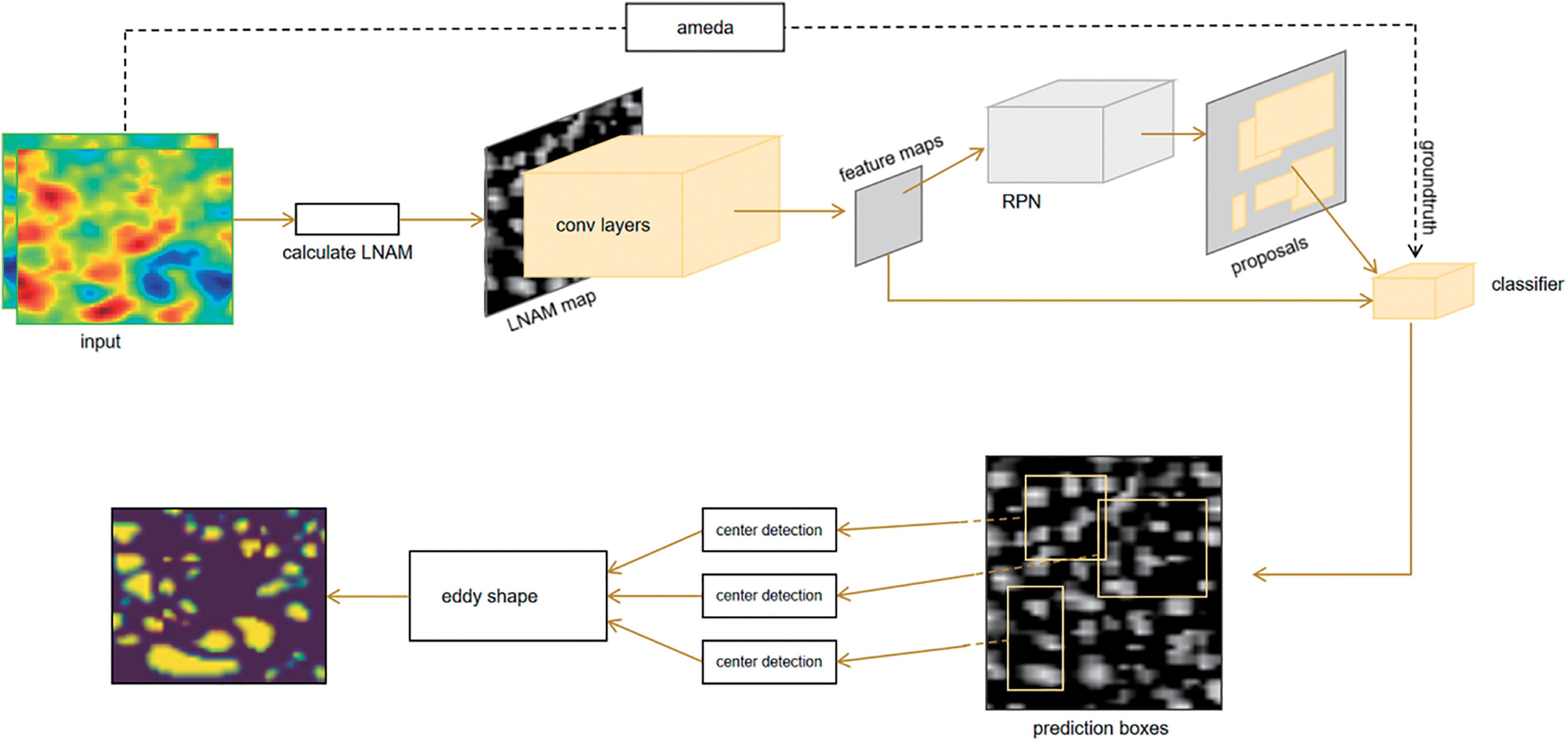
Figure 1: The architecture of our eddy detection model

3.2.1 Calculate LNAM

LNAM is a physical parameter introduced by Mkhinini et al. [16], denoting the integral of angular momentum across the surface area of the sea. This metric attains its peak value at the central point Gi, of the eddy. For every grid point Gi, LNAM is computed using the subsequent formula:

LNAM(Xi)=∑jXiXj×Vj∑jXiXj⋅Vj+∑j|XiXj|⋅|Vj|=LiSi+BLi(1)

Here, Xi signifies the longitude and latitude coordinates of the grid point Gi, while Vi represents the velocity vector of the sea surface surrounding this point. By constructing a square with a side length of Lb from the grid point’s center, the angular momentum at that specific location is then calculated as the integral of the cross product of the position vector and the sea surface velocity vector within the square area, projected onto the grid point as:

Li=∑j(GjXj×Vj)(2)

LNAM is a physical quantity proportional to the local angular momentum, and it normalizes the angular momentum through:

BLi=∑j|GjXj|⋅|Vj|(3)

This value is the upper bound of the angular momentum. Then add Si=∑j(GjXj⋅Vj) to the renormalization term. The sum of scalar products Si will reach a maximum value at hyperbolic points and equal zero at elliptic points. For an axisymmetric eddy, when Gi represents the eddy center, Si equals zero, and the LNAM parameter will reach an extremal value of 1 (or −1) for a cyclonic (or anticyclonic) eddy.

Here, we use LNAM as the input for training and prediction in Faster R-CNN. Compared to using parameters like SSH, UGOS, and VGOS alone, LNAM is a dynamic parameter that better describes local angular momentum. In Faster R-CNN, the feature extraction network initially converts the input multi-channel image into a single-channel image. This means that even if we place different pieces of information such as SSH, UGOS, and VGOS in different channels of the image, the feature extraction network will average the information from each channel, making it difficult to effectively extract key features from different channels of information. LNAM, on the other hand, integrates multidimensional information from physics. Using LNAM as input helps the feature extraction network extract key information about eddies, making the proposal boxes generated by the Region Proposal Network more accurate. Then, the classifier comprehensively extracts features to identify the content in the proposal boxes as eddy. With this approach, there will be fewer omissions or misjudgments in the bounding boxes, and the coordinates and sizes of the bounding boxes for the same eddy compared to the ground truth will be closer. In summary, using LNAM as input for Faster R-CNN improves the accuracy of eddy boxes.

3.2.2 Faster R-CNN Based Eddy Bounding Box Detection

Our bounding boxes generation module consists of two modules. The first module is a deep fully convolutional network used to propose boxes may containing eddies called proposals. The second module identifies eddies within the proposals based on feature maps extracted from LNAM.

Feature extraction networks are typically deep convolutional networks such as ResNet [35] and VGG [36]. As shown in Fig. 2, we take LNAM single-channel images with dimensions ranging from 50 × 50 pixel to 100 × 100 pixel as input and extract dynamic features of ocean surfaces through multiple layers of convolution and pooling. These features are then shared with subsequent Region Proposal Network (RPN) and ROI classifiers.

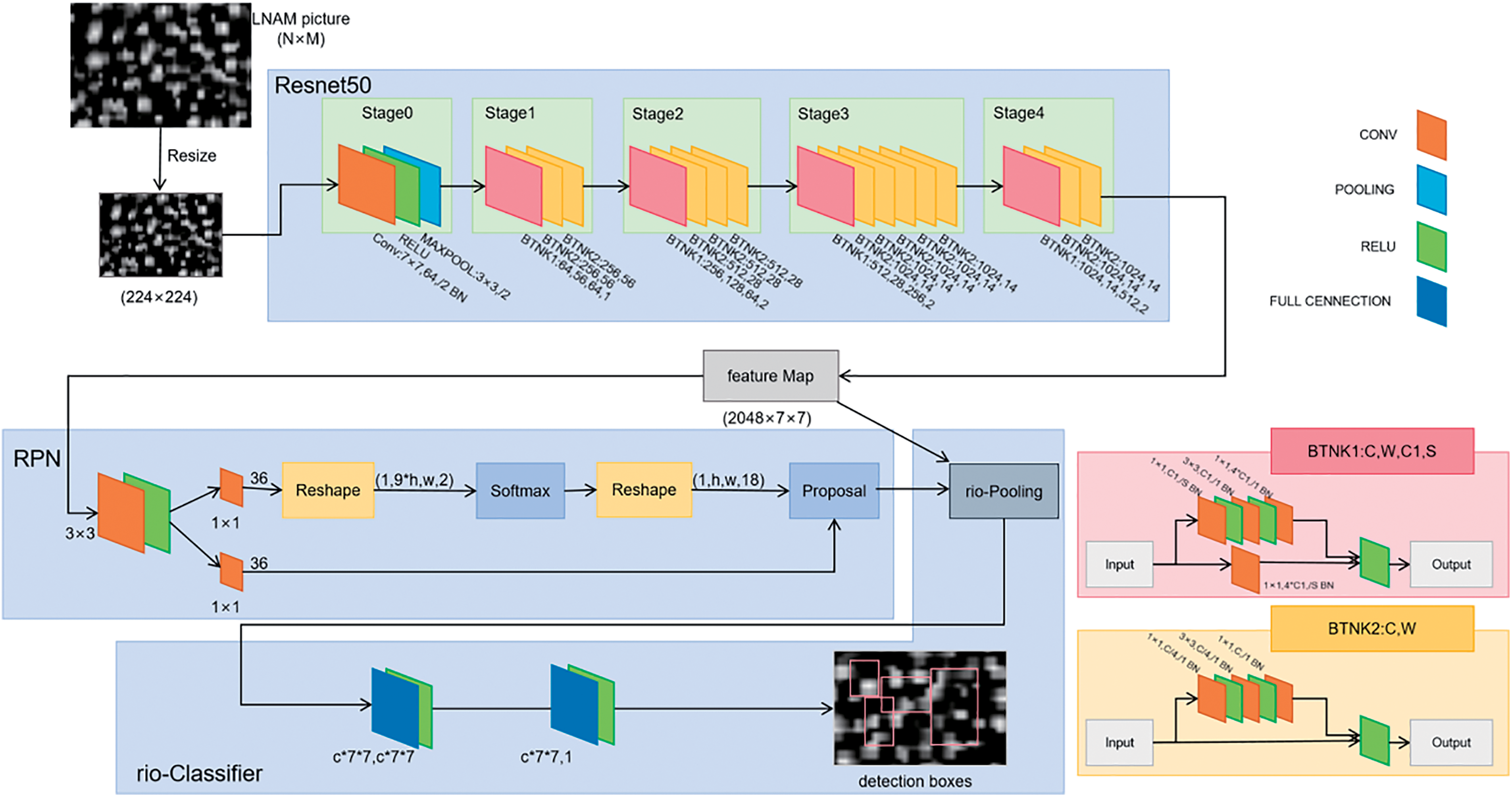
Figure 2: The architecture of bounding boxes generation model

In the Region Proposal Network (RPN), firstly, the goal is to output approximately 2000 rectangular-shaped anchor boxes, each with a score indicating the probability of containing a eddy. We model this process using a fully convolutional network. A small network slides over the feature map, taking an n × n window as input. Features within this window are extracted, and the anchor boxes along with their scores are obtained through this small network.

To reduce computation and avoid multiple identifications of the same eddies, we perform some simple filtering on these anchor boxes. All anchor boxes generated by RPN from an LNAM image are sorted by score in descending order. Boxes with low scores are removed, followed by the removal of overlapping boxes with large intersection areas. The remaining boxes are proposals. The number of proposals depends on the actual number of eddies in the input image, generally ranging from 50 to 300 pixels.

In the ROI classifier, we first make the proposal boxes pass through the ROI-Pooling layer [37], utilizing the feature maps within the boxes to adjust their positions and sizes. Then they are fed into the classifier for further identification of eddies. Finally, among all the adjusted proposal boxes, we select some proposals with higher probabilities as the bounding boxes for identifying eddies.

During the training process, we create a bounding box for each eddy detected in the AMEDA results, treating it as the ground truth. We then continuously adjust the parameters of the entire network model through backpropagation to make it approach the detection results of AMEDA.

• Loss of Network

To train the network, we assign labels to each anchor box generated by the RPN. For a given anchor, if it satisfies either condition, then we consider it a positive sample:

(i)   which is having the highest IoU (Intersection over Union) overlap with a ground truth box, or condition.

(ii)   which is having an IoU overlap higher than 0.7 with any ground truth box.

If IoU ratio of a given anchor with all ground truth boxes is less than 0.3, then we consider it a negative sample.

Anchors that do not fall into either category are neither positive nor negative samples and do not influence the training objective, so we do not include them in the loss calculation. Based on these definitions, the loss function defined for an image is as follows [30]:

L({pi}, {ti})=1Ncls∑iLcls(pi, pi∗)+λ1Nreg∑ipi∗Lreg(ti, ti∗)(4)

Lreg(ti, ti∗)=R(ti−ti∗)(5)

Lcls represents is log loss over two classes. R represents the robust loss function (smooth L1) [30]. pi represents the probability that the network predicts the i-th anchor to be an eddy. For positive samples, pi∗=1, and for negative samples, pi∗=0. ti represents the parameterized coordinate eddy, indicating the offset between the predicted box and the anchor box, and ti∗ represents the corresponding ground truth, indicating the offset between the ground truth box and the anchor box. Ncls is the size of the mini-batch, and Nreg is the number of anchor positions. λ is a constant used to balance the sum of the two losses.

3.2.3 AMEDA

• Center Detection

In center detection, we first input the entire LNAM map, and then consider each bounding box one by one. We extract the LNAM region corresponding to the bounding box to obtain LNAM’, and then draw contours on LNAM’ to calculate the extremum of LNAM. However, the mere presence of LNAM extremum does not ensure that the chosen eddy center accurately identifies the core area surrounding the water mass. Therefore, it’s essential to pinpoint a center where closed streamlines are observed around it. Subsequently, within a square region with the identified extremum as the center and a diameter of 10Rd, we compute the local stream function from the velocity field. In the case of the AVISO dataset, AMEDA can utilize contour lines of ADT and/or streamlines of the geostrophic velocity field directly as the local stream function.

If we intend to apply AMEDA to a submesoscale turbulent eddy field where the eddy radius is significantly smaller than the local deformation radius Rd, then it’s necessary to adjust the parameter Lb accordingly. However, in the scenario of geostrophic and mesoscale eddies resulting from the instability of coastal currents, it’s believed that setting Lb to approximately 1.2 times Rd brings us close to the optimal value for eddy center detection.

• Eddy Shape

At this stage, we interpolate the characteristic eddy contour using an ellipse and determine an equivalent ellipticity ε=1−a1/a2, also known as the flattening parameter, where a1 represents the semiminor axis and a2 represents the semimajor axis. To disregard highly distorted contours, we also calculate the local curvature along each streamline. If more than 20% of the streamline perimeter exhibits relative negative curvature, then the streamline is excluded from the analysis and cannot be utilized as a characteristic contour. Additionally, to filter out large gyres that may form at the basin scale, corresponding to the path or loop of semipermanent regional currents, we set a limit on the size of the characteristic contours such that Rmax≤Rlim. For the AVISO dataset, this limit is fixed at Rlim=59Rd≃50∼100 km, whereas for idealized numerical simulations or laboratory experiments, it is set at half the size of the numerical domain or the laboratory tank.

3.3 Computational Complexity Analysis

At this stage, we will analyze the complexity of the method proposed in this article. We use S to represent the area of the map to be detected.

In the traditional AMEDA algorithm, it is necessary to calculate the data around each grid point in LNAM. That is to say, when calculating each grid point, a constant level of computation will be generated, which we denote as O(k1). Therefore, the complexity of calculating LNAM is O(k1S).

In center detection, AMEDA needs to create contour lines for the input LNAM, and the number of contour lines is positively correlated with S. For each contour line, geometric processing needs to be performed at every position on the input grid data. Assuming the complexity of processing each point is O(k2). So, the overall complexity of center detection is O(k2S2).

In eddy shape, AMEDA needs to process the contour of each eddy. During this process, information around the eddy center needs to be considered, and multiple iterations need to be performed. We can use O(k3) to represent the complexity required for each eddy in eddy shape. k3 can be determined by many parameters and is a relatively large constant. Because the number of eddies is positively correlated with S, the total complexity of eddy shape is O(k3S).

So, the total complexity of AMEDA is O(k1S+k2S2+k3S).

In our approach, which we denote as O(k4S). We use Faster R-CNN to generate bounding boxes of eddies, and center detection only needs to be performed within these bounding boxes of eddies. Because the area of these generated bounding boxes often does not exceed 300, which is much smaller than S, the complexity of performing center detection separately for all bounding boxes is

O(k2∑isi2)≤O(k2×300∑isi)≈O(300k2S)(6)

Since 300 is significantly smaller than S and the computation time of Faster R-CNN is proportional to S, we can consider its complexity as O(k4S). Therefore, we can obtain the complexity of this article’s method as O(k1S+k4S+k3S).

It can be seen that from the analysis of complexity, the complexity of the method proposed in this article is superior to the traditional AMEDA algorithm.

4  Experiment

4.1 Setup

The computer hardware and software configuration for model training and prediction include: -NVIDIA RTX 4090 graphics card-Intel(R) Core (TM) i7-13700F CPU-64 GB RAM-Windows 11 22H2 operating system-Python 3.10.13 interpreter-NumPy 1.26.0-PyTorch 2.1.0. For the Faster R-CNN model used in this paper, we trained it with 3000 images, and each epoch step takes about 20 min. We use the AdamW Optimizer with parameters learning_rate=0.01, β1=0.9, β2=0.999.

4.2 Metrics

4.2.1 IoU

Intersection over Union (IoU) is a commonly used metric in the field of object detection. In the field of object detection, it measures the accuracy of detection by calculating the IoU between the detection box and the ground truth box. It is defined by the following equation:

IoU=B1∩B2B1∪B2(7)

B1 and B2 are two rectangular boxes, B1∩B2 represents their area of intersection, and B1∪B represents their area of union. IoU values range between 0 and 1, in the field of object detection, with higher values indicating better detection accuracy. Typically, IoU values above 0.70 or 0.80 are considered indicative of highly accurate detections.

Here, we use IoU to measure the similarity of two eddy contours.

However, since the shape of an eddy is typically a polygon, calculating the intersection and union of two polygons’ areas is a complex task. To simplify the computation, we approximate the intersection over union (IoU) of two polygons by randomly sampling 1000 points. Then, we can obtain:

IoU=Peddy1∧eddy2Peddy1∨eddy2(8)

In which Peddy1∧eddy2 represents the number of points falling into both eddy1 and eddy2 simultaneously, and Peddy1∨eddy2 represents the number of points falling into either eddy1 or eddy2.

4.2.2 Eddy Recognition Error

In evaluating the accuracy of detection results, if the IoU of a eddy detected by the method proposed in this paper with a eddy detected by AMEDA is greater than 0.8, then we consider this eddy to be valid. Within a certain region, the ratio of undetected eddy to eddies detected by AMEDA is termed as the eddy recognition error E, which is calculated as follows:

E=1−NvilidNameda(9)

E varies range from 0 to 1. A smaller E indicates fewer errors or omissions in eddy recognition, leading to better recognition performance.

4.2.3 RMSE of Eddy Centers

Root Mean Square Error (RMSE) is a metric for the accuracy of a model’s predictions. It represents the average deviation between predicted values and actual values, with smaller values indicating better performance. The formula for RMSE is as follows:

RMSE=1n∑i(yi−yi′)2(10)

Then we use RMSE to measure the deviation of the eddy center.

4.3 Result

4.3.1 Loss of Network

In this section, we use ADT, UGOS, and VGOS data from AVISO to train the Faster R-CNN model. The experimental data is selected from 2 January, 2000, in the region from 123.25°E to 167.75°E longitude and 11.75°N to 54.75°N latitude, with a resolution of 0.25°. Since the training target area is larger compared to the input area of the model, we randomly extract 3000 small regions with sizes ranging from 15 × 15 pixel to 25 × 25 pixel from this area, and then enlarge them by four times in both width and height using interpolation to create jpg images.

Here we use images of different types of information as inputs to evaluate the impact of different input information on Faster R-CNN’s detection results.

We divide the experiments into three groups:

The first group uses single-channel images made from SSH as inputs for training.

In the second group, we put SSH, UGOS, and VGOS into the RGB channels respectively, create three-channel images, and use these three-channel images as inputs for training.

In the third group, we calculate LNAM based on UGOS and VGOS, and use single-channel images made from LNAM as inputs for training.

After 30 rounds of training, their changes are shown in Table 1 and Fig. 3.

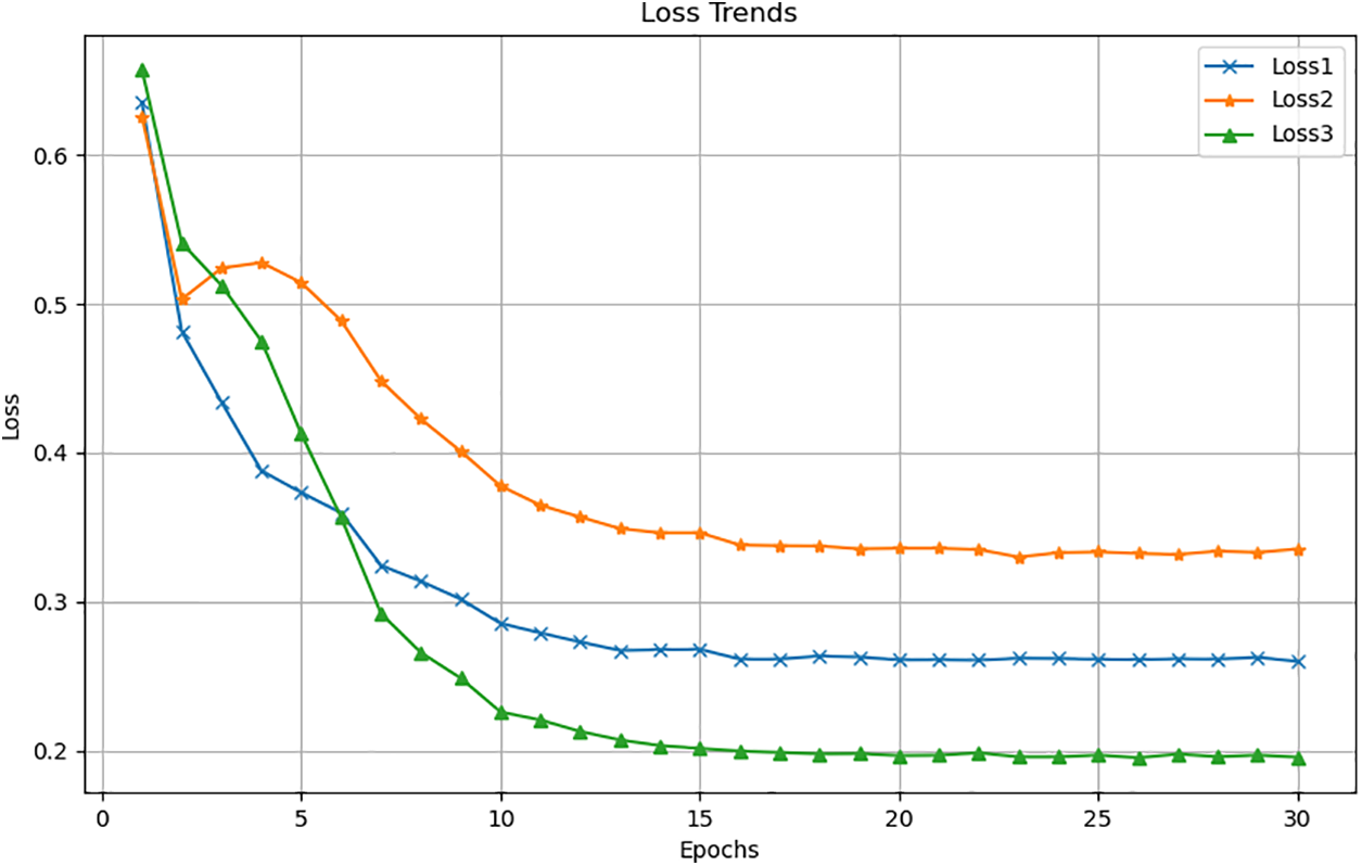
Figure 3: Trends of loss

4.3.2 Error of Eddy Detection and RMSE of Centers

In this section, to inspect the accuracy of the detection results of the proposed method, we conducted comparative experiments. The first group employed the traditional AMEDA algorithm, while the second group utilized our method. Additionally, to verify the superiority of bounding boxes generated using the Faster R-CNN network architecture, we designed a third group of experiments. In this group, we removed the Faster R-CNN module from our method and directly applied a sliding window approach on the original data to generate bounding boxes of size 30 × 30 pixel. To remove the impact of box edges, we set the sliding window stride to 15, meaning adjacent bounding boxes would overlap by 15 units in length. Finally, we also established the fourth group, using EddyNet for recognition, to compare the effectiveness of a purely machine learning approach.

The Fig. 4 shows a part of the experimental area that we extracted, which are [−76.25 W, −4.25 W] × [−60.25 S, 1.25 N], [−164.25 W, −94.25 W] × [−64.25 S, 6.25 N], and [−101.25 W, −31.25 W] × [−1.25 S, 69.25 N]. From the image, it can be observed that the results of the second and third groups are similar to the first group, while the results of the fourth group are significantly different. It is evident that the second and third groups are based on the AMEDA method, and their results are relatively close to each other. However, in the EddyNet of the fourth group, pure machine learning methods cannot identify well. Furthermore, in the training of EddyNet, it can only be trained for a specific area, such as region (1). Therefore, the EddyNet trained in this way can only detect eddies in that particular region. If a trained network is used to identify other regions, such as (2) and (3), the recognition performance will be much lower. Thus, EddyNet has almost no generalization ability for eddy recognition, whereas the second and third groups based on AMEDA are suitable for eddy recognition in various regions and have strong generalization ability.

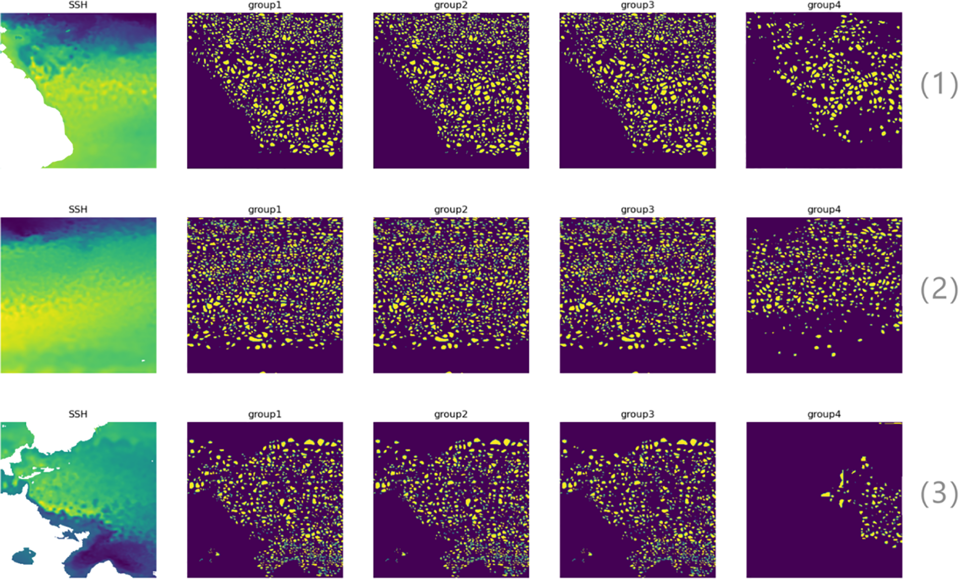
Figure 4: The test results of each group. Yellow color block indicates eddies had been detected

Next, we will select a portion of the Fig. 5, with the region [−58.25 W, −36.25 W] × [−52.25 S, −29.25 S], to zoom in and compare the recognition results.

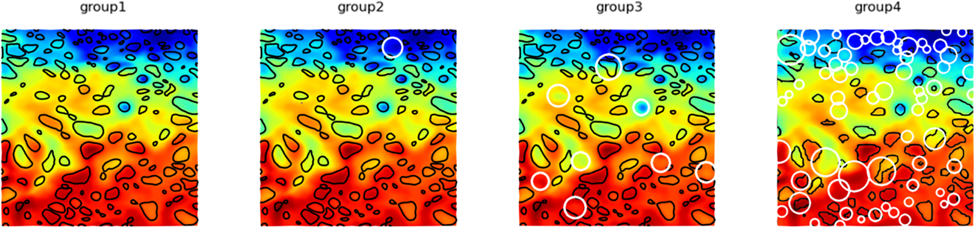
Figure 5: Detailed result. White circles indicating errors detected

As seen from the above figure, both the second group and the third group have difference compared to the first group, but the difference in the second group is much smaller compared to the difference in the third group. As for the fourth group, although the selected area is within the training area of EddyNet, the detection results are also very different from AMEDA.

Hs is a parameter in AMEDA that directly influences the number of contours. The quantity of contours affects the accuracy of eddy detection. A larger Hs results in more contours, which makes the boundaries of detected eddies more precise and facilitates the identification of smaller eddies. Conversely, smaller Hs values lead to fuzzier eddy boundaries and may result in missing some smaller eddies. Next, for groups one, two, and three, we will conduct more detailed experiments in larger ocean areas using different Hs parameters. The Hs values we choose 40, 120 and 200.

The experimental areas are shown in the Table 2 below.

As shown in Fig. 6, in the above experiments for the three values of Hs, AMEDA respectively identified 9156, 9826, and 9973 eddies. The number of correctly identified eddies in group two is 9051, 9763, and 9908, while in group three, it is 8349, 9088, and 9277. It can be seen that under different parameters and different areas, the number of correctly identified eddies in group two is always bigger than that in group three.

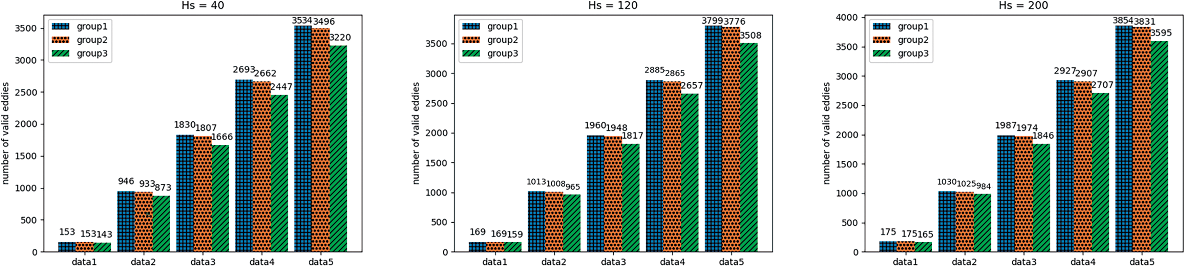
Figure 6: The number of valid eddies

As shown in Fig. 7, among the five areas and three Hs values, the eddy identification error in group two is generally around 0.01, while in group three, it is all above 0.06, more than 6 times greater than in group two.

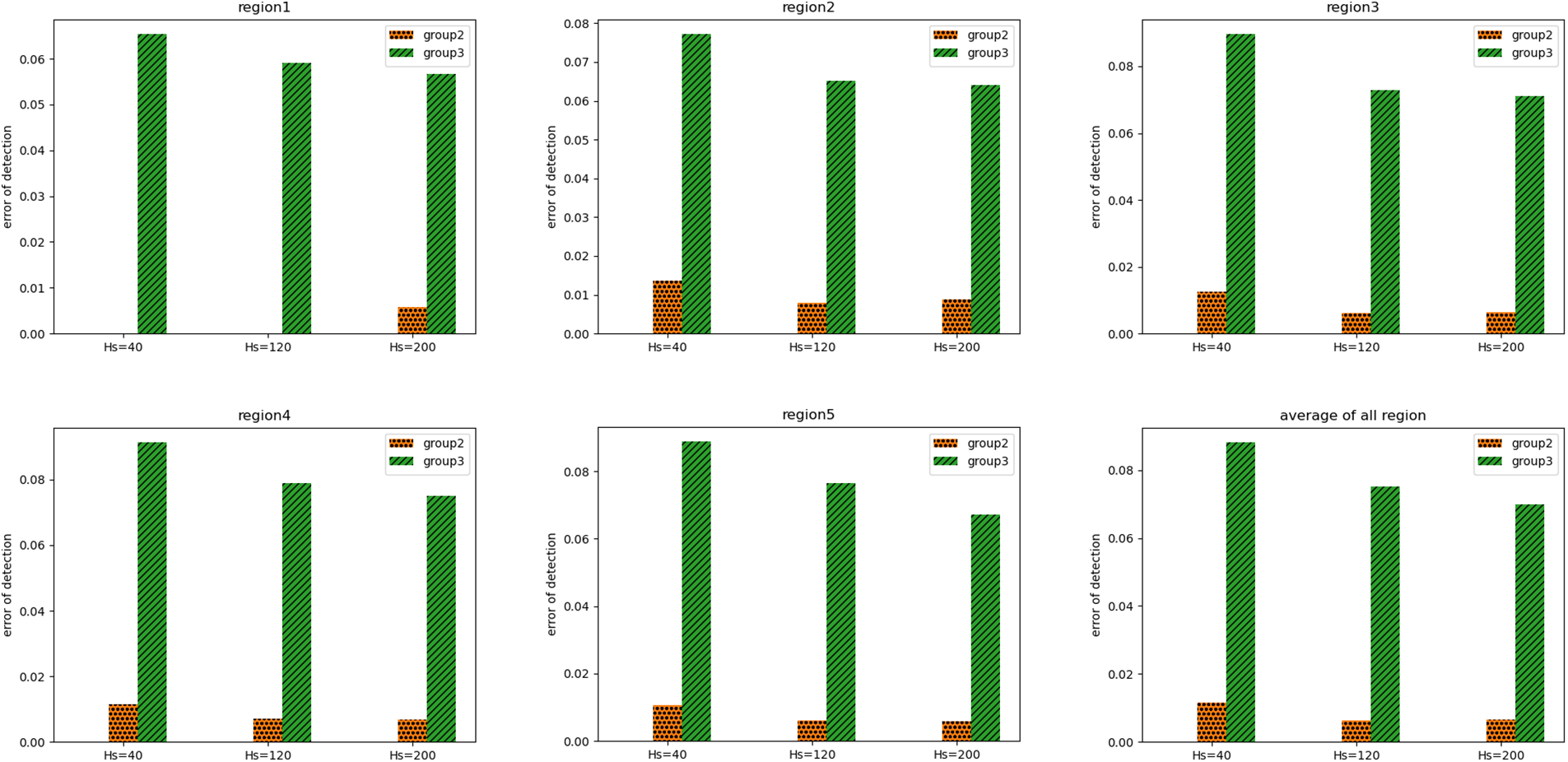
Figure 7: The error of detection in each region. The 6-th one is the average error of all regions

In the Fig. 8, we plotted the horizontal and vertical coordinate differences between the center of each recognized eddy and the center of AMEDA’s on a two-dimensional plane. It can be seen that for various values of Hs, compared to the third group, the second group has more points clustered at the origin. Next, we calculated the RMSE of the center of each group’s eddies with AMEDA’s eddies and compiled the Table 3.

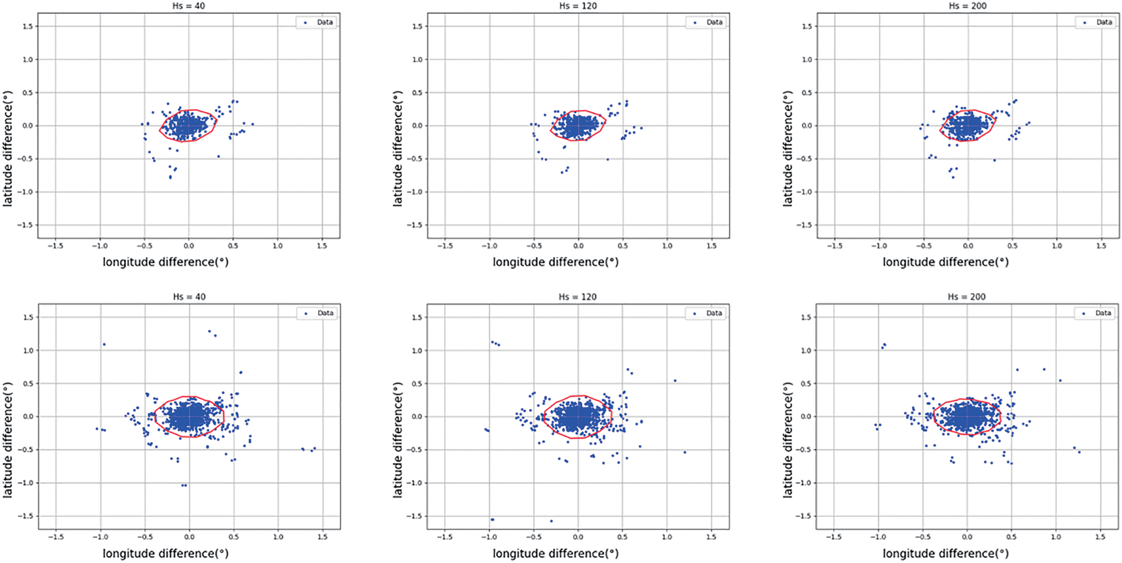
Figure 8: Error of each center of eddies. Red contour includes 90% points

According to Table 3, the RMSE of eddy centers in group two is mostly around 0.0025, which is also much smaller than in group three. In conclusion, the eddies detected by the method in this article are not significantly different from those detected by the original AMEDA method, and the bounding boxes extracted by the target detection model are clearly superior.

4.3.3 Running Time

In this section, we designed experiments similar to the first three groups of experiments in Section 4.2.2. As a representative, we set the parameter Hs = 20 and conducted tests on eight datasets of different sizes.

We define the relative area of the experimental region as the product of the longitude range size and the latitude range size, denoted as |lon1−lon2|⋅|lat1−lat2|.

As shown in Table 4, we selected 8 regions for testing, presenting their corresponding latitude and longitude ranges, as well as their relative areas. Each region is identified by a letter (A to H). The latitude range indicates the extent from the southernmost point (−85.25°S) to the northernmost point (either positive or negative), while the longitude range spans from the westernmost point (−185.25°W) to the easternmost point (either positive or negative). The relative area column quantifies the size of each region, providing a comparative measure of their spatial extents.

In these three sets of experiments, the actual running times of AMEDA in experimental areas A and H were 32 and 5100 s, respectively, while the running times of the our method in areas A and H were 29 and 1345 s, respectively. According to Fig. 9, it can be seen that when the input area is small, the differences in running time among the three groups are very small; however, when the area is large, AMEDA’s running time will be much higher than that of the method described in this paper.

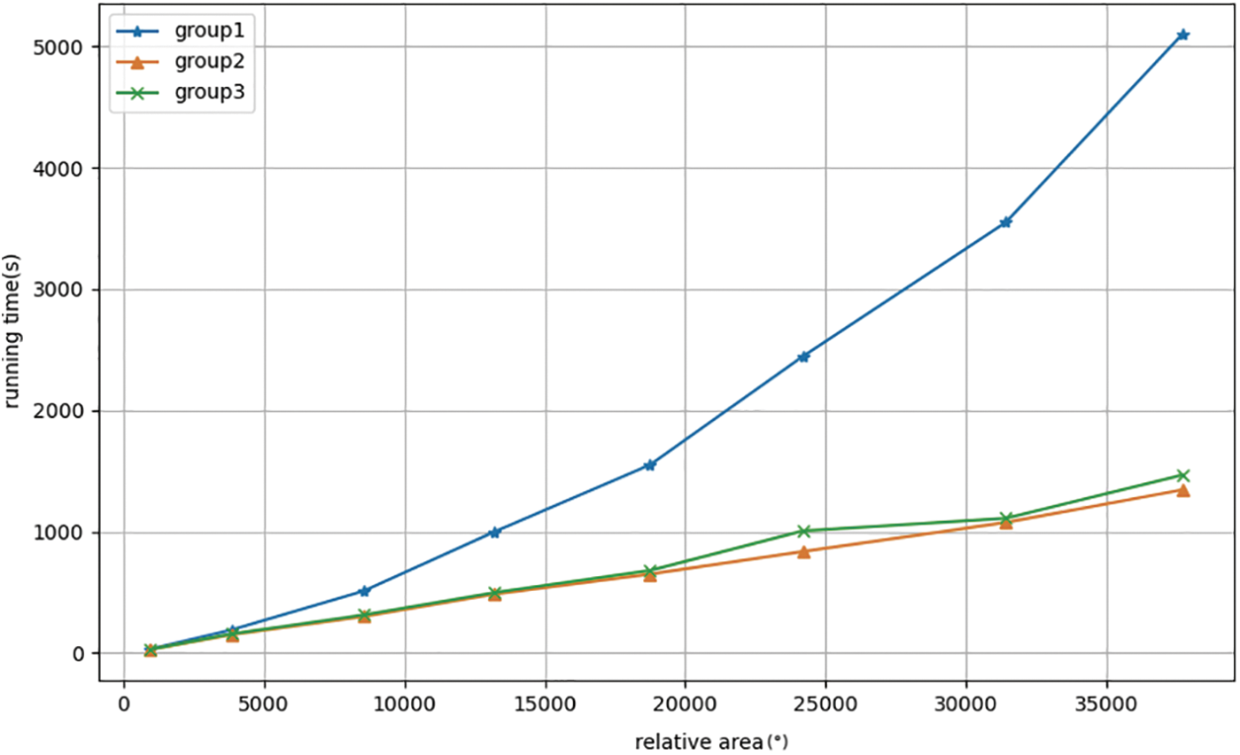
Figure 9: Running time of each groups

In Fig. 10, the growth rate of AMEDA’s running time appears to be a linear function related to the input area, so AMEDA’s running time is linearly correlated with the square of the input area; while the growth rate of our method remains consistent everywhere, within the range of 0.025 to 0.050, so the running time of the method described in this paper is linearly correlated with the input area.

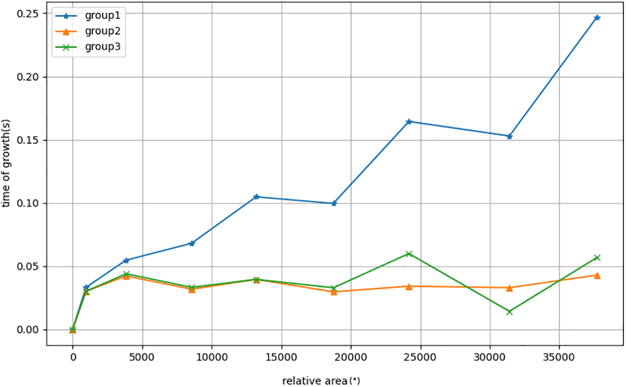
Figure 10: Growth rate of running time

On the other hand, in Section 3.3, we analyzed the complexities of AMEDA and our method, which are respectively O(k1S+k2S2+k3S) andO(k1S+k4S+k3S). It can be seen that our complexity analysis is consistent with the running time in the experiments. Through differentiation of the complexities, it can be known that AMEDA’s complexity grows at a linear rate, while the complexity of the method described in this paper grows at a constant rate. This is also consistent with our experimental results.

5  Conclusion

In this paper, we propose a solution for detecting eddies, which integrates the Faster R-CNN object detection model and the traditional AMEDA method, addressing the shortcomings of traditional methods in detection efficiency and the low accuracy of many pure deep learning methods. We use Faster R-CNN to detect bounding boxes of generated eddies, allowing AMEDA to detect eddy centers within these bounding boxes, and then unify eddy shapes.

We conducted comparative experiments on different regions based on the AVISO dataset: compared to eddyNet, the detection results of this method are closer to AMEDA. In each experimental group, the identification error compared to AMEDA does not exceed 2%, and the RMSE of eddy centers is around 0.002.

Through complexity analysis, we found that the complexity of our method in this paper is O(k1S+k4S+k3S), while the complexity of the AMEDA algorithm is O(k1S+k2S2+k3S). From the complexity analysis, we can conclude that our method in this paper is more efficient than AMEDA. According to our experiments, in smaller experimental areas, the speed difference between the two is not significant, while in global-scale prediction experiments, the detection time is one-fourth of AMEDA’s.

However, there are still some problems to be solved in the future. In AMEDA, the computational cost of the eddy shape module is very high. After reducing the complexity of center detection in this paper, eddy shape has become the bottleneck of computational efficiency. In the future, it may be possible to accelerate shape computation by integrating information around eddy centers through methods similar to eddyNet and other deep learning approaches.

Acknowledgement: The author sincerely thanks the National Science Foundation of China and the National Natural Science Foundation of China for providing funding support to the laboratory.

Funding Statement: The authors extend their appreciation to the National Science Foundation of China (No. 42175194) and the National Natural Science Foundation of China (No. 41976165) for funding this work.

Author Contributions: Xinchang Zhang: Conceptualization, Investigation. Xiaokang Pan: Writing original draft, Study conception and design. Rongjie Zhu: Data collection, Data curation. Runda Guan: Writing original draft. Zhongfeng Qiu: Analysis and interpretation of results. Biao Song: Supervision, Study conception and design. All authors reviewed the results and approved the final version of the manuscript.

Availability of Data and Materials: The datasets generated during and/or analyzed during the current study are available in this link: https://www.aviso.altimetry.fr/ (accessed on 5 June 2023).

Ethics Approval: Not applicable.

Conflicts of Interest: The authors declare that they have no conflicts of interest to report regarding the present study.

References

1. Chen G, Yang J, Han G. Eddy morphology: egg-like shape, overall spinning, and oceanographic implications. Remote Sens Environ. 2021;257:112348. [Google Scholar]

2. McWilliams JC. The nature and consequences of oceanic eddies. Geophys Monogr Series. 2008;177:5–15. [Google Scholar]

3. Morrow R, Le Traon PY. Recent advances in observing mesoscale ocean dynamics with satellite altimetry. Adv Space Res. 2012;50(8):1062–76. [Google Scholar]

4. Wunsch C. Where do ocean eddy heat fluxes matter? J Geophys Res: Oceans. 1999;104(C6):13235–49. [Google Scholar]

5. Koshlyakov MN, Belokopytov VN. Mesoscale eddies in the open ocean: review of experimental investigations. Phys Oceanogr. 2020;27(6):559–72. [Google Scholar]

6. Cabrera M, Santini M, Lima L, Carvalho J, Rosa E, Rodrigues C, et al. The southwestern Atlantic ocean mesoscale eddies: a review of their role in the air-sea interaction processes. J Mar Syst. 2022;235:103785. [Google Scholar]

7. Chen G, Yang J, Tian F, Chen S, Chen S, Zhao C, et al. Remote sensing of oceanic eddies: progresses and challenges. Natl Remote Sens Bull. 2021;25:302–22. [Google Scholar]

8. Huo J, Zhang J, Yang J, Li C, Liu G, Cui W. High kinetic energy mesoscale eddy identification based on multi-task learning and multi-source data. Int J Appl Earth Obs Geoinf. 2024;128:103714. [Google Scholar]

9. Nencioli F, Dong C, Dickey T, Washburn L, McWilliams JC. A vector geometry-based eddy detection algorithm and its application to a high-resolution numerical model product and high-frequency radar surface velocities in the Southern California bight. J Atmos Oceanic Technol. 2010;27(3):564–79. [Google Scholar]

10. Le VUB, Stegner A, Arsouze T. Angular momentum eddy detection and tracking algorithm (AMEDA) and its application to coastal eddy formation. J Atmos Oceanic Technol. 2018;35(4):739–62. [Google Scholar]

11. Xu G, Xie W, Dong C, Gao X. Application of three deep learning schemes into oceanic eddy detection. Front Mar Sci. 2021;8:672334. [Google Scholar]

12. Lguensat R, Sun M, Fablet R, Tandeo P, Mason E, Chen G. EddyNet: a deep neural network for pixel-wise classification of oceanic eddies. In: 2018 IEEE International Geoscience and Remote Sensing Symposium (IGARSS), 2018; Valencia, Spain; IEEE; p. 1764–7. [Google Scholar]

13. Duo Z, Wang W, Wang H. Oceanic mesoscale eddy detection method based on deep learning. Remote Sens. 2019;11(16):1921. [Google Scholar]

14. Zi N, Li XM, Gade M, Fu H, Min S. Ocean eddy detection based on YOLO deep learning algorithm by synthetic aperture radar data. Remote Sens Environ. 2024;307:114139. [Google Scholar]

15. Ren S, He K, Girshick R, Sun J. Faster R-CNN: towards real-time object detection with region proposal networks. IEEE Trans Pattern Anal Mach Intell. 2016;39(6):1137–49. [Google Scholar] [PubMed]

16. Mkhinini N, Coimbra ALS, Stegner A, Arsouze T, Taupier-Letage I, Beranger K. Long-lived mesoscale eddies in the eastern Mediterranean Sea: analysis of 20 years of AVISO geostrophic velocities. J Geophys Res: Oceans. 2014;119:8603–26. [Google Scholar]

17. Ducet N, Le Traon PY, Reverdin G. Global high-resolution mapping of ocean circulation from TOPEX/Poseidon and ERS-1 and -2. J Geophys Res: Oceans. 2000;105(C8):19477–98. doi:10.1029/2000JC900063. [Google Scholar] [CrossRef]

18. Le Traon PY, Nadal F, Ducet N. An improved mapping method of multisatellite altimeter data. J Atmos Oceanic Technol. 1998;15(2):522–34. doi:10.1175/1520-0426(1998)015<0522:AIMMOM>2.0.CO;2. [Google Scholar] [CrossRef]

19. Okubo A. Horizontal dispersion of floatable particles in the vicinity of velocity singularities such as convergences. Deep Sea Res Oceanogr Abstr. 1970;17(3):445–54. doi:10.1016/0011-7471(70)90059-8. [Google Scholar] [CrossRef]

20. Weiss J. The dynamics of enstrophy transfer in two-dimensional hydrodynamics. Physica D: Nonlinear Phenomena. 1991;48(2–3):273–94. doi:10.1016/0167-2789(91)90088-Q. [Google Scholar] [CrossRef]

21. Chelton DB, Schlax MG, Samelson RM. Global observations of nonlinear mesoscale eddies. Progress in Oceanogr. 2011;91(2):167–216. doi:10.1016/j.pocean.2011.01.002. [Google Scholar] [CrossRef]

22. Chaigneau A, Gizolme A, Grados C. Mesoscale eddies off Peru in altimeter records: identification algorithms and eddy spatio-temporal patterns. Prog Oceanogr. 2008;79(2–4):106–19. [Google Scholar]

23. Zhang C, Li H, Liu S, Shao L, Zhao Z, Liu H. Automatic detection of oceanic eddies in reanalyzed SST images and its application in the East China Sea. Sci China Earth Sci. 2015;58(12):2249–59. [Google Scholar]

24. Xing T, Yang Y. Three mesoscale eddy detection and tracking methods: assessment for the South China Sea. J Atmos Oceanic Technol. 2021;38(2):243–58. [Google Scholar]

25. Yu C, Wang J, Peng C, Gao C, Yu G, Sang N. BiSeNet: Bilateral segmentation network for real-time semantic segmentation. In: Proceedings of the European Conference on Computer Vision, 2018; Munich, Germany; p. 325–41. [Google Scholar]

26. Sun X, Zhang M, Dong J, Lguensat R, Yang Y, Lu X. A deep framework for eddy detection and tracking from satellite sea surface height data. IEEE Trans Geosci Remote Sens. 2020;59(9):7224–34. [Google Scholar]

27. Chen LC, Papandreou G, Schroff F, Adam H. Rethinking atrous convolution for semantic image segmentation. arXiv preprint arXiv:1706.05587. 2017. [Google Scholar]

28. Saida SJ, Ari S. Automatic detection of ocean eddy based on deep learning technique with attention mechanism. In: Proceedings of NCC, 2022; Mumbai, India; IEEE; p. 302–7. [Google Scholar]

29. Saida SJ, Ari S. Dilated convolution based U-Net architecture for ocean eddy detection. In: Proceedings of SILCON, 2022; Silchar, India; IEEE; p. 1–5. [Google Scholar]

30. Saida SJ, Ari S. MU-Net: modified U-Net architecture for automatic ocean eddy detection. IEEE Geosci Remote Sens Lett. 2022;19:1–5. [Google Scholar]

31. Zhao Y, Fan Z, Li H, Zhang R, Xiang W, Wang S, et al. SymmetricNet: end-to-end mesoscale eddy detection with multi-modal data fusion. Front Mar Sci. 2023;10:1174818. [Google Scholar]

32. Santana OJ, Hernández-Sosa D, Martz J, Smith RN. Neural network training for the detection and classification of oceanic mesoscale eddies. Remote Sens. 2020;12(16):2625. [Google Scholar]

33. Santana OJ, Hernández-Sosa D, Smith RN. Oceanic mesoscale eddy detection and convolutional neural network complexity. Int J Appl Earth Obs Geoinf. 2022;113:102973. [Google Scholar]

34. Pegliasco C, Chaigneau A, Morrow R, Dumas F. Detection and tracking of mesoscale eddies in the Mediterranean Sea: a comparison between the sea level anomaly and the absolute dynamic topography fields. Adv Space Res. 2021;68(2):401–19. [Google Scholar]

35. Koonce B, Koonce B. ResNet 50. Convolutional neural networks with swift for tensorflow: image recognition and dataset categorization. Sebastopol, CA, USA: Apress; 2021. p. 63–72. [Google Scholar]

36. Simonyan K, Zisserman A. Very deep convolutional networks for large-scale image recognition. arXiv preprint arXiv:1409.1556. 2014. [Google Scholar]

37. Girshick R. Fast R-CNN. In: Proceedings of the IEEE International Conference on Computer Vision, 2015; Santiago, Chile; p. 1440–8. [Google Scholar]