
 Submit a Paper
 Propose a Special lssue
 Open Access
ARTICLE
Three-Dimensional Multiferroic Structures under Time-Harmonic Loading
1 Department of Civil Engineering, National Yang Ming Chiao Tung University, Hsinchu, 300, Taiwan
2 Disaster Prevention and Water Environment Research Center, National Yang Ming Chiao Tung University, Hsinchu, 300, Taiwan
3 Department of Applied Science, Krishna Institute of Engineering and Technology, Ghaziabad, 201206, India
* Corresponding Authors: Sonal Nirwal. Email: ; Ernian Pan. Email:
Computer Modeling in Engineering & Sciences 2024, 141(2), 1165-1191. https://doi.org/10.32604/cmes.2024.054255
Received 23 May 2024; Accepted 12 August 2024; Issue published 27 September 2024
 View Full Text
 Download PDF
Abstract
Magneto-electro-elastic (MEE) materials are a specific class of advanced smart materials that simultaneously manifest the coupling behavior under electric, magnetic, and mechanical loads. This unique combination of properties allows MEE materials to respond to mechanical, electric, and magnetic stimuli, making them versatile for various applications. This paper investigates the static and time-harmonic field solutions induced by the surface load in a three-dimensional (3D) multilayered transversally isotropic (TI) linear MEE layered solid. Green’s functions corresponding to the applied uniform load (in both horizontal and vertical directions) are derived using the Fourier-Bessel series (FBS) system of vector functions. By virtue of this FBS method, two sets of first-order ordinary differential equations (i.e., N-type and LM-type) are obtained, with the expansion coefficients being Love numbers. It is noted that the LM-type system corresponds to the MEE-coupled P-, SV-, and Rayleigh waves, while the N-type corresponds to the purely elastic SH- and Love waves. By applying the continuity conditions across interfaces, the solutions for each layer of the structure (from the bottom to the top) are derived using the dual-variable and position (DVP) method. This method (i.e., DVP) is unconditionally stable when propagating solutions through different layers. Numerical examples illustrate the impact of load types, layering, and frequency on the response of the structure, as well as the accuracy and convergence of the proposed approach. The numerical results are useful in designing smart devices made of MEE solids, which are applicable to engineering fields like renewable energy.Keywords
In recent years, smart composite materials have found applications in ultrasonic imaging devices, space structures, and energy harvesting [1–4]. These smart materials are capable of altering their dimensions, shape, rigidity, and various mechanical properties when exposed to external temperature, electric field, mechanical field, and others.
Among the smart materials, multiferroic or magneto-electro-elastic (MEE) materials have energy conversion capacities [5]. While single-phase multiferroics have only weak magnetoelectric (ME) coupling, materials composed of piezoelectric (PE) and piezomagnetic (PM) phases can have strong ME coupling for converting energy from one form into another [6–8]. Their capacity to convert and manipulate energies makes them useful in diverse fields. From innovative sensors capable of detecting subtle changes in magnetic (or electric) fields to actuators designed to respond dynamically to external stimuli, these materials become important in diverse engineering fields. Their role in developing advanced transducers, efficient energy harvesting systems, and even cutting-edge medical devices underscores their significance in shaping the future of technology and engineering [9–11]. Malleron et al. [12] conducted an experimental study on magnetoelectric transducers for powering small biomedical devices. Li et al. [13] investigated the static behaviour of MEE materials in a hygrothermal environment using the multi-physical cell-based smoothed finite element method (MCS-FEM). Their study highlights the significance of employing MCS-FEM for solving multi-physical problems. Sasmal et al. [14] reviewed recent progress in flexible magnetoelectric composites and devices for next-generation wearable electronics, focusing on strategic fabrication techniques to improve the performance of flexible ME composites and devices.
To fully exploit the potential of these advanced materials, it is essential to accurately model their behaviour under various conditions. One of the most effective tools for this purpose is the fundamental solution, also called Green’s functions (GF). GFs are pivotal in various analytical and numerical techniques [15–17] as they provide a means to solve complex boundary-value problems involving different classes of materials such as MEE materials. Given the intricate coupling among magnetic, electric, and elastic fields in MEE solids, accurate determination and utilization of GFs become crucial. They help in understanding and predicting how these materials will respond to different stimuli, which is essential for designing applications [18–20]. For instance, in the development of advanced transducers and sensors, GFs enable precise calculations and optimizations necessary for high performance. This importance is particularly evident when smart materials are used in layered structures. The complexity of these structures requires precise solutions to boundary-value problems, which GFs can provide. Yang et al. [21] investigated the natural characteristics of anisotropic MEE multilayered plates using the analytical and finite element approach and drew their conclusion on three-layered plates with four different stacking sequences. Guided wave propagation in a multilayered MEE curved panel by the Chebyshev spectral elements method was discussed by Xiao et al. [22]. Vattree et al. [23] studied the semicoherent heterophase interfaces in 3D MEE multilayered composites under external loads. The appropriate structural interface conditions and the corresponding complicated boundary-value problem were solved using the mathematically elegant and computationally powerful Stroh formalism combined with the Fourier transform and dual-variable and position method (DVP). Singularity-free theory and adaptive finite element computations of arbitrarily shaped dislocation loop dynamics in 3D heterogeneous material structures are described by Vattré et al. [24]. Small-scale thermal analysis of piezoelectric–piezomagnetic Functionally Graded (FG) microplates using modified strain gradient theory was carried out by Hung et al. [25]. Kiran [26] studied thermal and hygrothermal buckling characteristics of porous magneto-electro-elastic skewed plates using third-order shear deformation theory. Additionally, Lyu et al. [27] conducted nonlinear dynamic modelling of geometrically imperfect MEE nanobeams made of functionally graded materials. Nonlinear isogeometric analysis of magneto-electro-elastic porous nanoplates was done by Phung et al. [28]. Circular loadings on the surface of an anisotropic and MEE half-space are investigated by Wang et al. [29]. Here, an analytical solution for a uniform and an indentation-type load is derived, distinguishing important features associated with the considered loadings. The different features of fracture analysis in PE and MEE materials are analyzed by Bui et al. [30] and Kiran et al. [31]. Various analytical and numerical methods have been proposed for solving the related problems in multilayered structures over the past decades [32–35]. In these studies, different real-life challenges such as imperfections, cracks, dynamic loads, and other factors are explored. These aspects are crucial when designing layered structures, as they significantly influence the performance and reliability of actual devices.
Previous studies have explored the essential nature of MEE multilayered structures. Although these investigations can extract the most essential nature of MEE multilayered structures, they were mostly limited to the static response under vertical loading, employing relatively complicated methods. However, the dynamic responses and real-world applications necessitate more sophisticated approaches, which GFs can facilitate. Understanding the dynamic behavior of MEE multilayered structures is crucial for their integration into modern technological systems. The ability to accurately predict and control their performance under various operational conditions can significantly improve the design and functionality of smart devices. GFs, with their advanced capabilities, provide a robust framework for modelling and analyzing these complex interactions.
In this paper, we analyze the time-harmonic response of 3D multilayered transversely isotropic (TI) MEE layered solids induced by arbitrary time-harmonic loads in both horizontal and vertical directions (including the electric load). While previous studies have primarily focused on the static response, understanding the time-harmonic response is important for many applications that involve dynamic and oscillatory loading conditions [36]. Time-harmonic loads are particularly important because they simulate real-world conditions where the materials are subjected to time-dependent forces, such as in ultrasonic imaging, vibration control, and energy harvesting systems [37]. Computing the time-harmonic response allows for the accurate prediction of transient behaviors and the dynamic interaction between magnetic, electric, and mechanical fields within MEE materials, which is vital for optimizing the performance and efficiency of devices.
Recent advancements in the fundamental solutions for layered structures, including the Fourier-Bessel series (FBS) vector function [38] and the DVP method [16], enhance the analytical precision in the study of MEE materials. The FBS and DVP methods exhibit computational efficiency and robustness, making them particularly advantageous for addressing complex dynamic problems. These methods facilitate the accurate modelling and analysis of transient behaviors in multilayered structures. The FBS system of vector function is attractive, with the decoupled solutions (LM- and N-type) in each layer being simply expressed by the eigenvalues and eigenvectors. Additionally, the DVP method is effective for handling layering due to its stability and efficiency. Furthermore, in terms of the FBS system, the solved coefficients are discrete Love numbers [39], which can be saved and repeatedly used on the surface of the layered solid. Since the GFs are just the summation of the Love numbers (multiplied by the given base functions), they can be accurately and fast calculated. In this paper, the GFs corresponding to the surface loading over a circular area will be derived in detail, with numerical examples showing the influence of loading types, frequencies and layering on the solutions.
The results of this study have applications in several engineering fields. Specifically, understanding the time-harmonic responses of MEE materials can significantly enhance the design and performance of devices subjected to dynamic and oscillatory loading conditions. For example, accurate modelling of time-harmonic responses in ultrasonic imaging can lead to better image resolution and deeper tissue penetration. In vibration control, improved response predictions can enhance the stability and effectiveness of damping systems. In energy harvesting systems, the ability to predict and optimize the dynamic interaction between different fields can lead to more efficient energy conversion and storage solutions. By addressing these practical applications, this research contributes to the advancement of smart material technologies and their integration into various high-performance engineering systems.
Fig. 1 depicts the 3D structure, which consists of an n-layered solid made of transversally isotropic (TI) -MEE solid materials. The Cartesian coordinate system (x, y, z) is attached to its (x, y)-plane on the surface and the layered solid in the positive z-direction. Each layer is ordered downward, with Layer 1 on the top (with z0 = 0). Layer j is bounded by two interfaces, z = zj–1 and z = zj, with thickness hj = zj –zj–1 (j = 1, ..., n). The last interface of Layer n, i.e., zn, rests on the homogeneous MEE half-space. We assume that the adjacent layers are perfectly bonded, and that the uniform time-harmonic loads in both vertical and horizontal directions are applied on the surface of the structure within a circular region of radius a (see Fig. 1). Since the loads are proportional to eiωt where ω = 2πf in Hz = 1/s is the angular frequency, the factor eiωt in the response will be omitted.
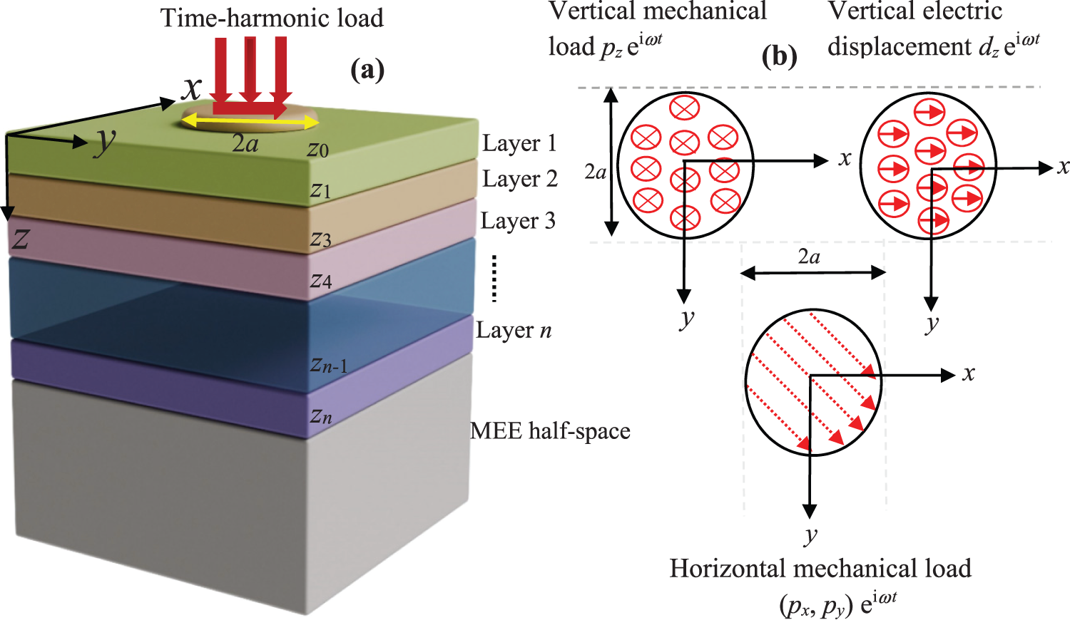
Figure 1: Schematic of the 3D structure composed of TI-MEE layered solid subjected to time-harmonic loads on its surface in (a), three types of time-harmonic loads, i.e., vertical mechanical load pz, vertical electric displacement dz and horizontal mechanical load (px, py) applied on the surface plane (x, y) of the structure within the circle of radius a in (b)
The problem presented above can be solved in terms of either Cartesian or cylindrical coordinate systems. Here, we employ the FBS vector system to solve the problem. Thus, the equations of motion and the Gauss law in the MEE solid without body forces, electric charge, and magnetic monopoles (proportional to eiωt) are given by [20]
where σij (N/m2) (i, j = r, θ, z) is mechanical stresses, Dj (C/m2) is electric displacement, and Bj (T = Wb/m2) is magnetic inductions; ρ (kg/m3) and ui (m) are mass density and elastic displacements.
The constitutive relation for TI-MEE materials (with its symmetry axis along z-axis) is given by [40]
where cij (N/m2), eij (C/m2), and εij (C2/N.m2) are the elastic moduli, PE tensor, and dielectric permittivity tensor, respectively; qij (N/A.m), dij (C/A.m), and μij (C2/N.m2) are the PM tensor, ME tensor and magnetic permeability tensor, respectively; γij (dimensionless), Ei (V/m) and Hi (A/m) are the strain tensor, electric field and magnetic field.
The strain components γij, electric field Ej and magnetic field Hj are related to the mechanical displacements ui, electric potential ϕ (V) and magnetic potential ψ (A) by [40]
2.2 Continuity Condition on any Interface
Since we have considered that the internal interfaces between layers are perfectly bonded, the mechanical displacements, electric potential, magnetic potential, tractions, electric displacements, and magnetic induction are continuous across it (e.g., at z = zk). Namely, we have
In the last homogeneous TI-MEE half-space, it is required that the solution remains finite.
2.3 Fundamental Solution in Terms of FBS System and DVP Method
2.3.1 FBS System of Vector Functions
To find the solution to the aforementioned boundary-value problem, the Fourier-Bessel series (FBS) vector functions are introduced [38]
where er, eθ and ez are the unit vectors along r-, θ-, and z-directions of the cylindrical system; λmk is the k-th zero of the Bessel function of order m, scaled by a large value R, i.e.,
The scalar function in Eq. (5) is defined by
which satisfies the following Helmholtz equation:
Due to the orthogonal property of the FBS system (i.e., Eq. (5)), u, ϕ and ψ can be expanded as [38]
Also, t (at z = constant plane), D and B can be expanded as [38]
where Um, Φ, Ψ, Tm, Dm, Bm (m = L, M and N) are the expansion coefficients. Notice that, upon determining these coefficients, the corresponding physical quantities can be obtained by taking the simple summation in Eqs. (8)–(13).
We now derive the ordinary differential equations for these expansion coefficients and their solutions. First, from the constitutive relations, we find
where a prime represents the derivative of the variable with respect to z.
Eqs. (14), (15a) and (16a) contain 10 expansion coefficients (i.e., UL, UM, UN, Φ, Ψ, TL, TM, TN, DL and BL) and need to be combined with the following 3 relations (from Eqs. (1)–(3)) to solve them
Now Eqs. (14), (15a), (16a) and (17) contain a total of ten equations for the ten coefficients. They can be converted into a linear system of first-order differential equations. Furthermore, both the LM-type and N-type systems are decoupled, with the N-type being purely elastic, as listed below:
where
and
Furthermore, the N-type solution is zero if the applied load is axis-symmetric.
Solutions of Eqs. (18) and (19) can be simply expressed in terms of their eigenvalues and eigenvectors. The general solution in any layer, say in Layer j bounded by zj-1 and zj, i.e.,
where
has a positive real part.
where [E] is the eigenmatrix and
with the first four eigenvalues (s1–s4) having positive real parts and the other four having negative real parts.
To find the solution in the multilayered TI-MEE solid, the DVP method is adopted. Thus, by following Pan et al. [38], we have the following layer relation:
where
In a similar manner, the expansion coefficients for Layer j+1 can be obtained. Thus, by assuming the continuity condition between the two adjacent layers (i.e., Eq. (4)), we can determine the recursive relation between Layer j and Layer j+1, which is given by
where
The recursive relation (i.e., Eq. (23)) can be repeatedly applied in structure as long as the interfaces between the layers are perfect.
2.3.4 Boundary Conditions on the Surface
The boundary condition at z = z0 (Fig. 1) (in terms of the Cartesian coordinate system and proportional to eiωt) is given by [38]
In terms of the FBS system, we have obtained the following coefficients due to the applied loads on the surface of the structure [38]
We consider the following three cases separately one by one here.
Case 1: Uniform vertical load pz. For this case, we have
Case 2: Uniform vertical electric displacement dz. For this case, we have
Case 3: Uniform horizontal load (px, py) in both x- and y-directions. For this case, we have
2.3.5 Expansion Coefficients on the Surface
With the surface traction coefficients, we apply the recursive relation for propagating the expansion coefficients from the surface z0 to the last layer interface zn to obtain the following relations:
On the last interface z = zn, the unknowns in Eq. (26) are related as
where Eij (Eij) are the eigenvector elements (submatrices) in the last MEE half-space.
Combined with Eq. (27), we can solve, from Eq. (26), the coefficients of displacements, electric potential, and magnetic potential on the surface of the layered structure, as given below.
Due to the applied vertical load (i.e., m = 0), we have only LM-type system, for which the expansion coefficients on the surface is given by
where
for the vertical mechanical load and vertical electric displacement, respectively.
Due to the applied horizontal load (i.e., for m =
and
where
Once the coefficients on the surface are obtained, we can find the solution at any point on the surface of the structure by carrying out the summation (i.e., Eqs. (8)–(13)). To find the solutions at any specific z level, we just need to replace z0 with z in Eq. (26). Since coefficients are discreet numbers, they represent the exact Love numbers [39]. These Love numbers are advantageous to simplify the computation process, as they can be pre-calculated and stored for repeated use in calculating the GFs [41].
3.1 Validation and Convergence of the Problem
Before presenting numerical results, the present field solutions are validated against existing ones and found to be consistent with the solution reported by Pan et al. [38], Chu et al. [40] and Qi et al. [42]. Fig. 2 illustrates the accuracy of the current method as compared with those of Chu et al. [40] and Qi et al. [42].
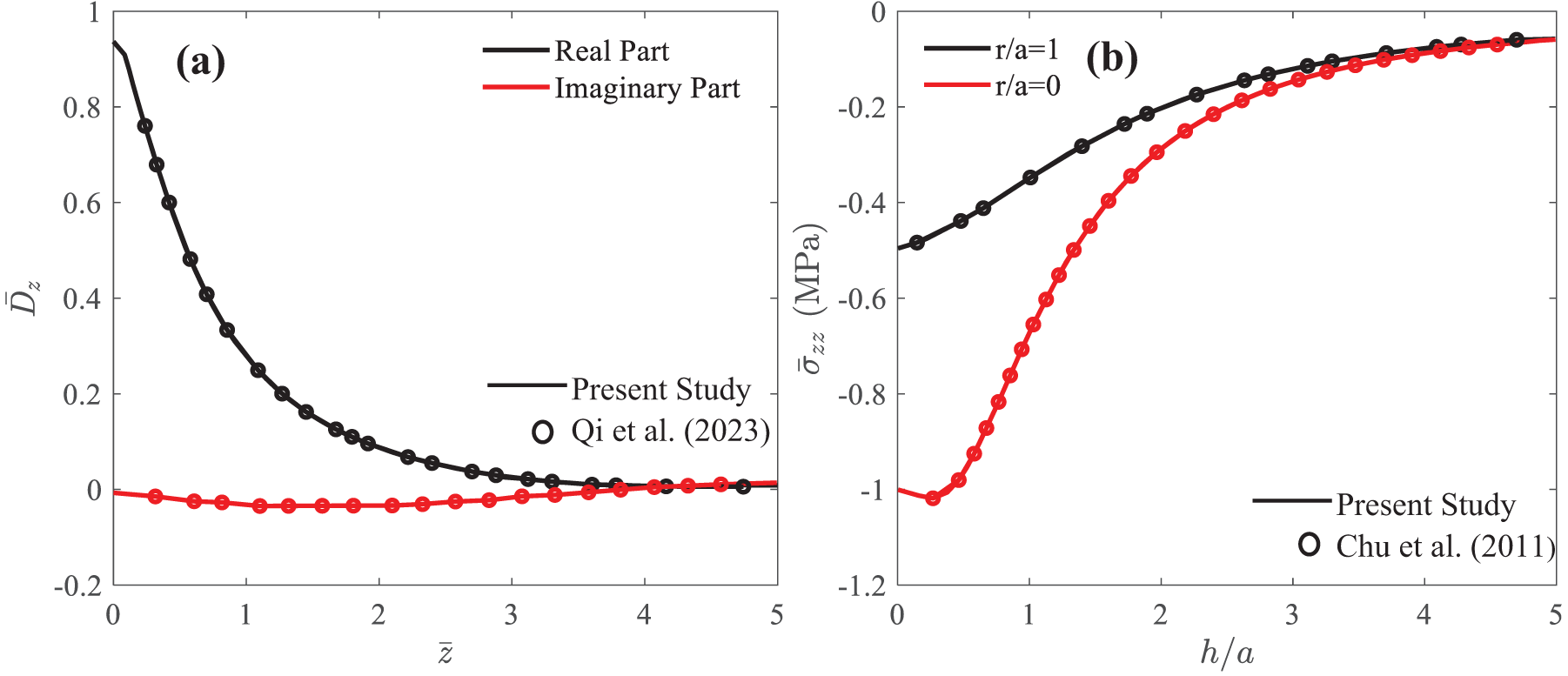
Figure 2: Variation of electric displacement
A loading radius of a = 1 nm is located on the surface with its center at the origin of the coordinate system. In the calculation, a small material damping factor, i.e., β = 0.0001, is applied to the material. Namely, ckj, ekj, qkj, ηkj, μkj and dkj are replaced by ckj (1 + 2iβ), ekj (1 + 2iβ), qkj (1 + 2iβ), ηkj (1 + 2iβ), μkj (1 + 2iβ) and dkj (1 + 2iβ) during the numerical computation. Furthermore, R in the FBS is fixed at 1500 nm (i.e., R = 1500 a) and M = 9000. In presenting the numerical findings in the paper, dimensionless parameters are used, as defined below.
where cmax, emax, and qmax are the maxima of the corresponding elastic, piezoelectric, piezomagnetic coefficients, and ρmax the maximum density, and ϕmax = emax/a and ψmax = qmax/a. The normalized electric and magnetic potentials are still dimensional variables.
Fig. 3 shows the surface displacements
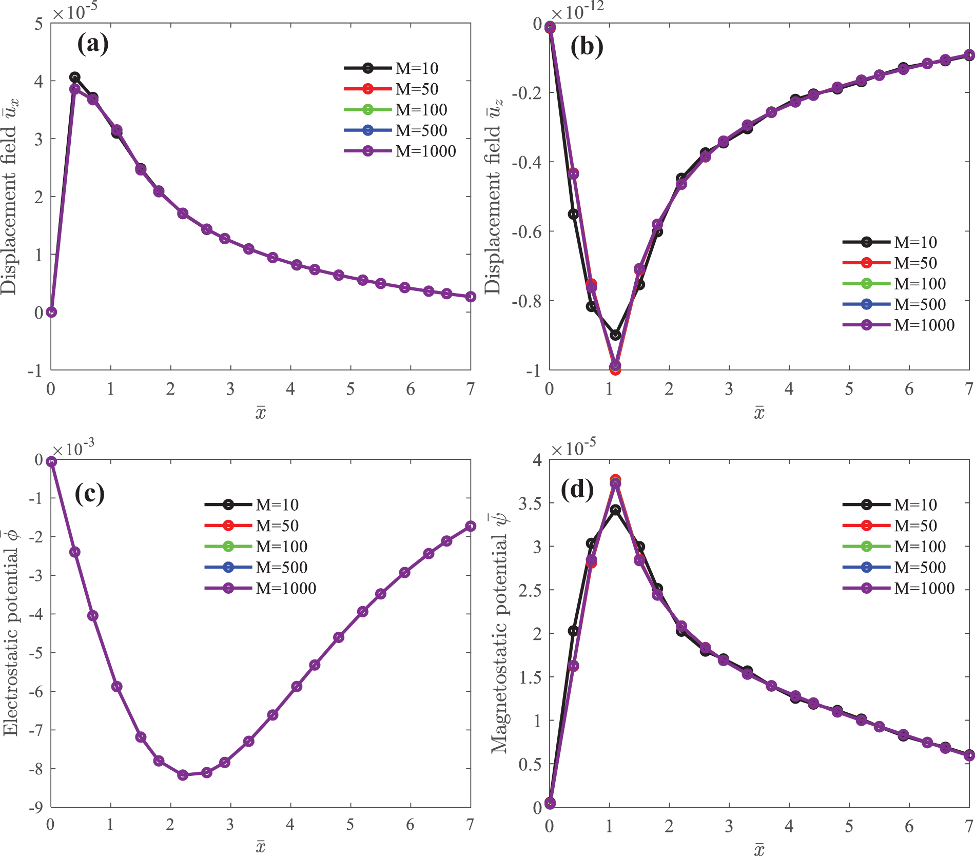
Figure 3: Surface elastic displacement
3.2 Time-Harmonic Loading on MEE Structures
Illustrative examples of the applied static and time-harmonic loads in nanoscale MEE multilayered structures are discussed in this section. The importance of layered structures in engineering lies in their capacity to offer tailored and multifunctional properties, making them pivotal in various applications. Understanding the dynamic behavior of MEE-layered structures and their distinct stacking configurations is essential for designing engineering structures with desired mechanical, electric, or magnetic characteristics, ensuring optimal performance in specific applications.
The proposed framework is applied to analyze the impact of vibration frequency and different configurations in half-space, bi-layered, tri-layered, and multilayered media. The structures are made of CoFe2O4 (magnetostrictive cobalt ferrite, CFO) and BaTiO3 (piezoelectric barium titanite, BTO), and their composite, i.e., 0.25, 0.50 and 0.75 BTO for which the properties of the material are taken from Vattré et al. [24].
3.2.1 Under Vertical Mechanical Loading
The static and time-harmonic responses due to the circular vertical mechanical load
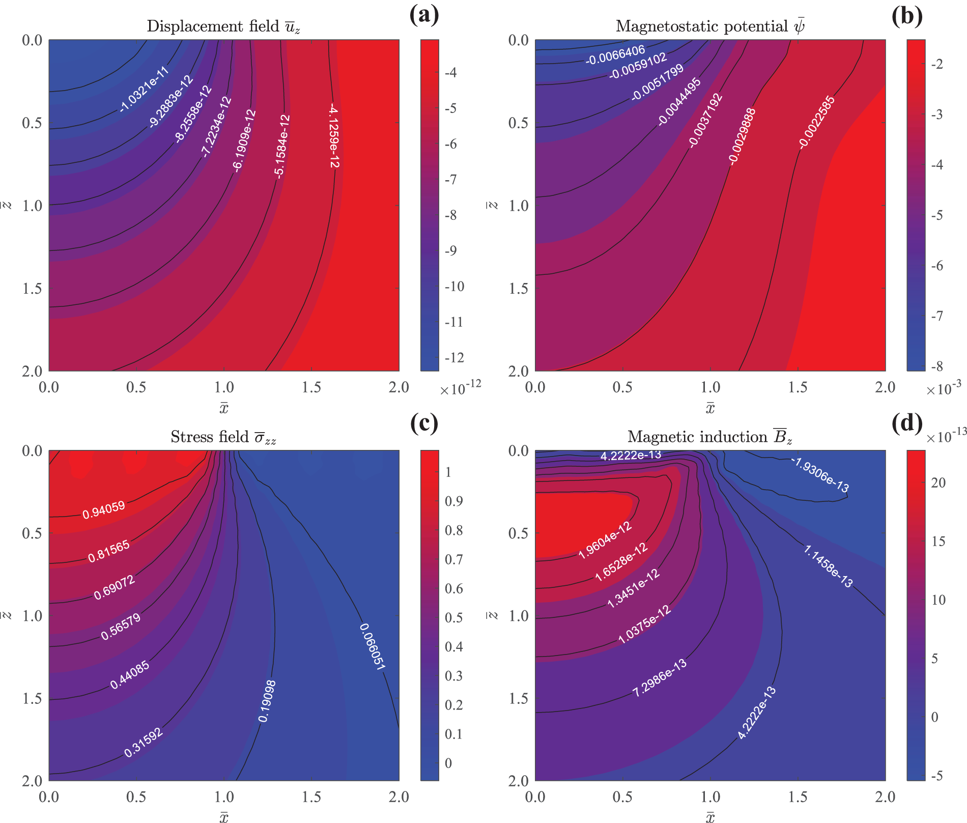
Figure 4: Contours of elastic displacement
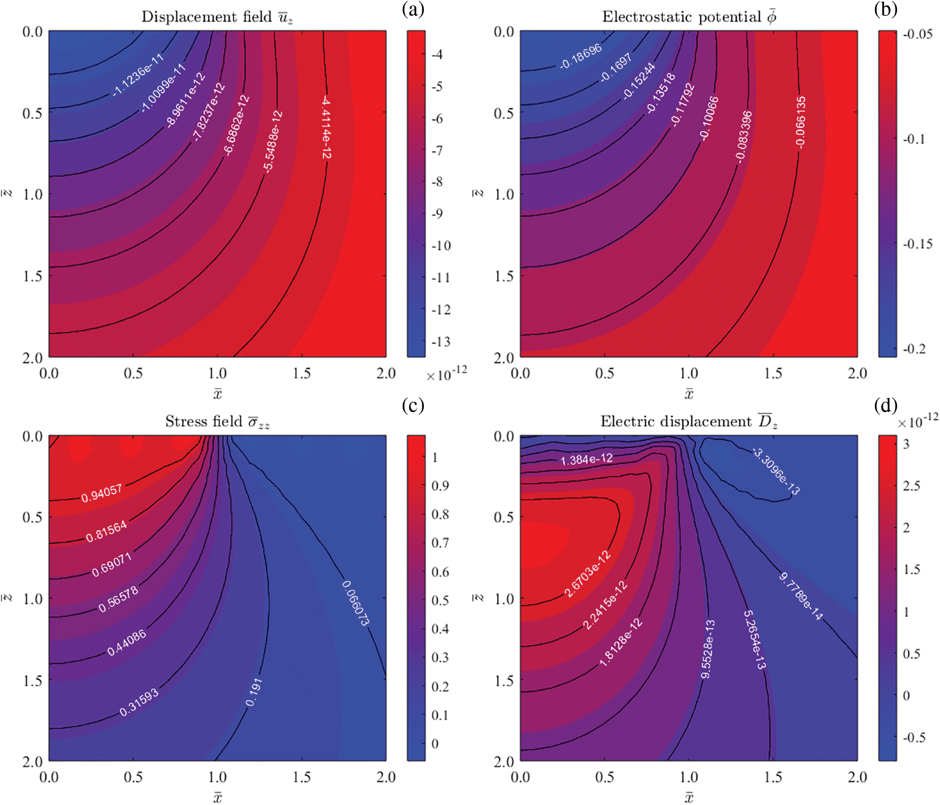
Figure 5: Contours of elastic displacement
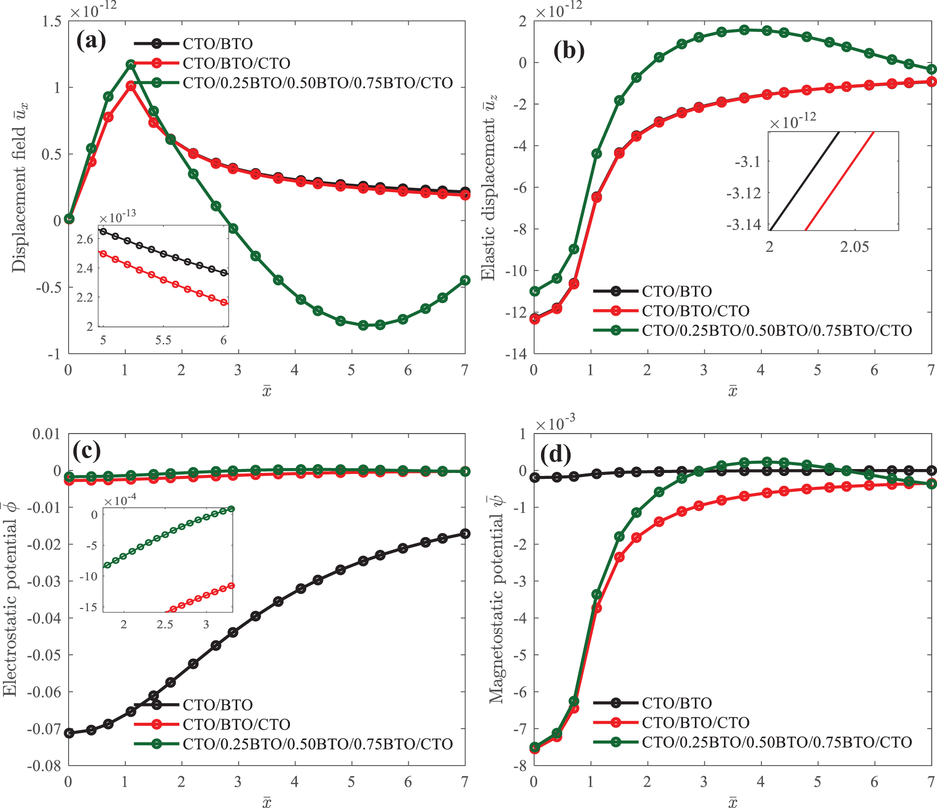
Figure 6: Elastic displacement
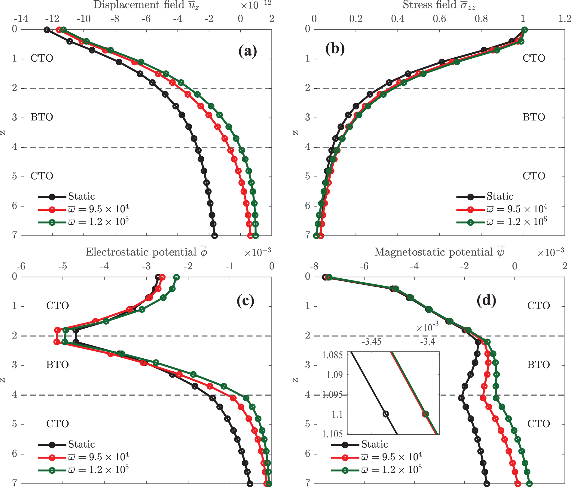
Figure 7: Effect of frequencies on elastic displacement
Fig. 4 presents the 2D contours of vertical elastic displacement
Fig. 6 illustrates the spatial distribution of field quantities on the surface, induced by the vertical mechanical load in CFO/BTO bi-layered, CFO/BTO/CFO tri-layered, and CFO/αBTO/CFO (α = 0.25, 0.50 and 0.75) multilayered structures. In Fig. 6a, it is noted that for 1 <
Fig. 7 shows the distribution of elastic displacement
3.2.2 Under Vertical Electric Displacement
The static and time-harmonic responses due to the circular vertical electric displacement
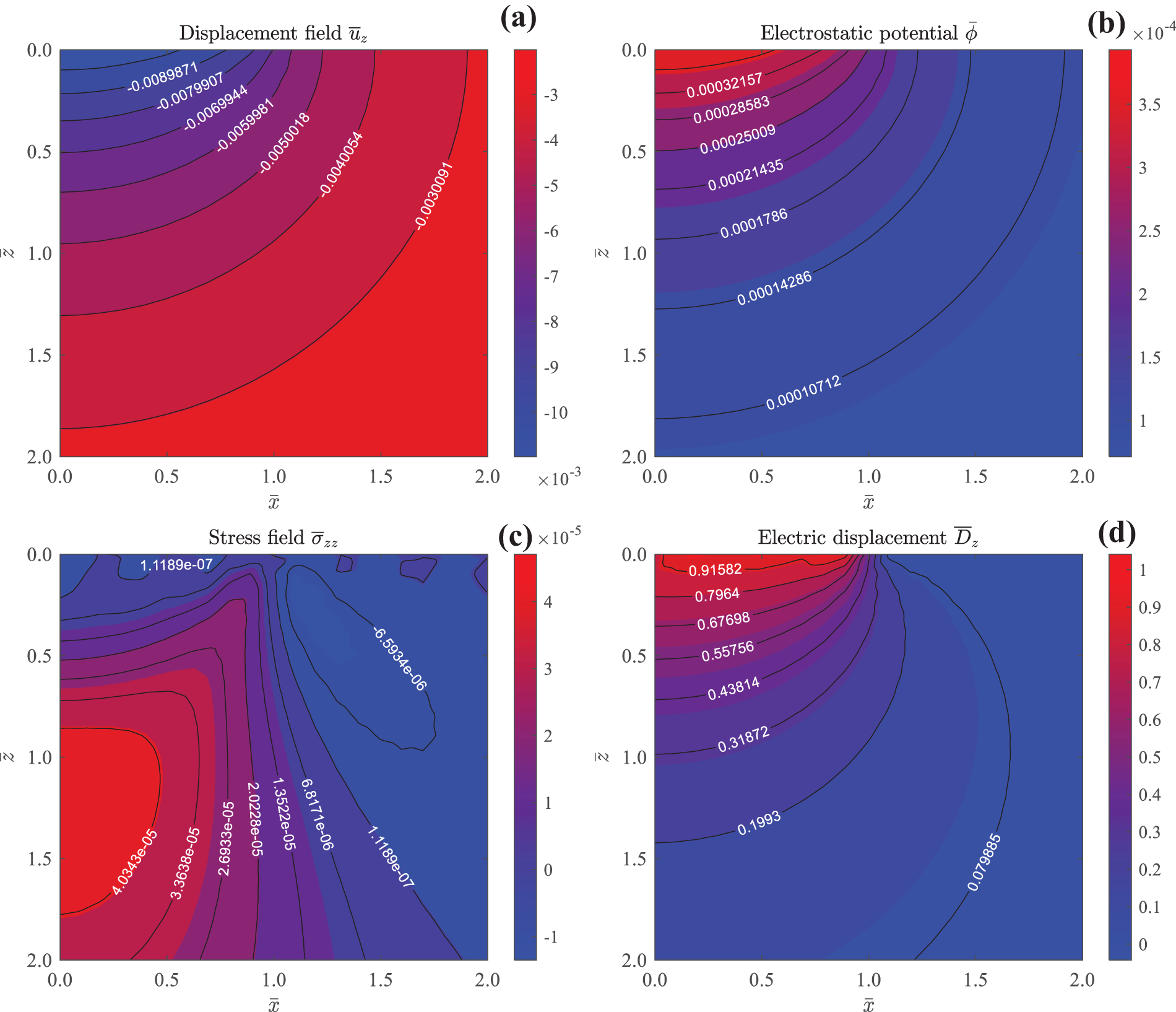
Figure 8: Contours of elastic displacement
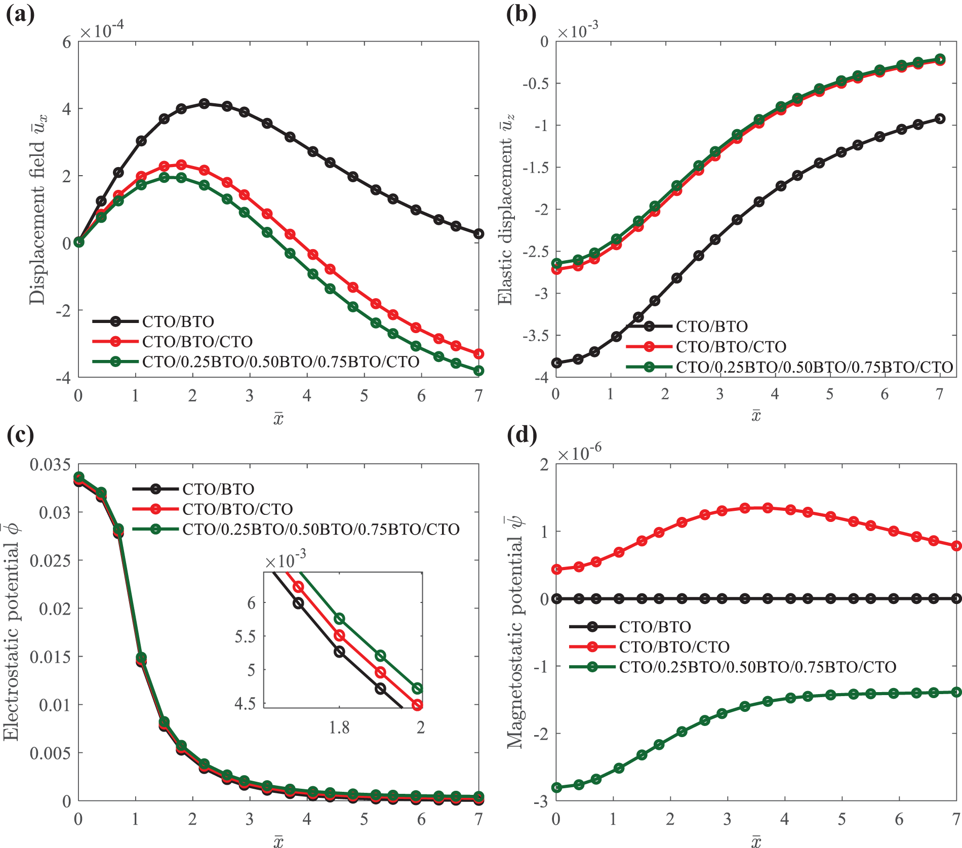
Figure 9: Surface elastic displacement
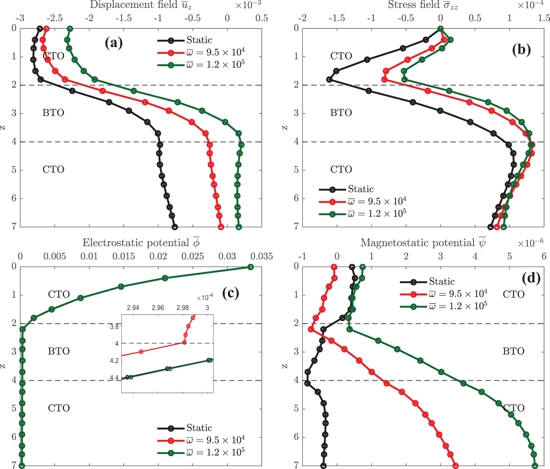
Figure 10: Effect of different frequencies on elastic displacement
Fig. 8 presents contours of elastic displacement
Fig. 9 illustrates the spatial distribution of elastic displacements
Fig. 10 shows how different frequencies (i.e.,
3.2.3 Under Horizontal Mechanical Loading
The static and time-harmonic responses of different layered structures subjected to circular horizontal mechanical load
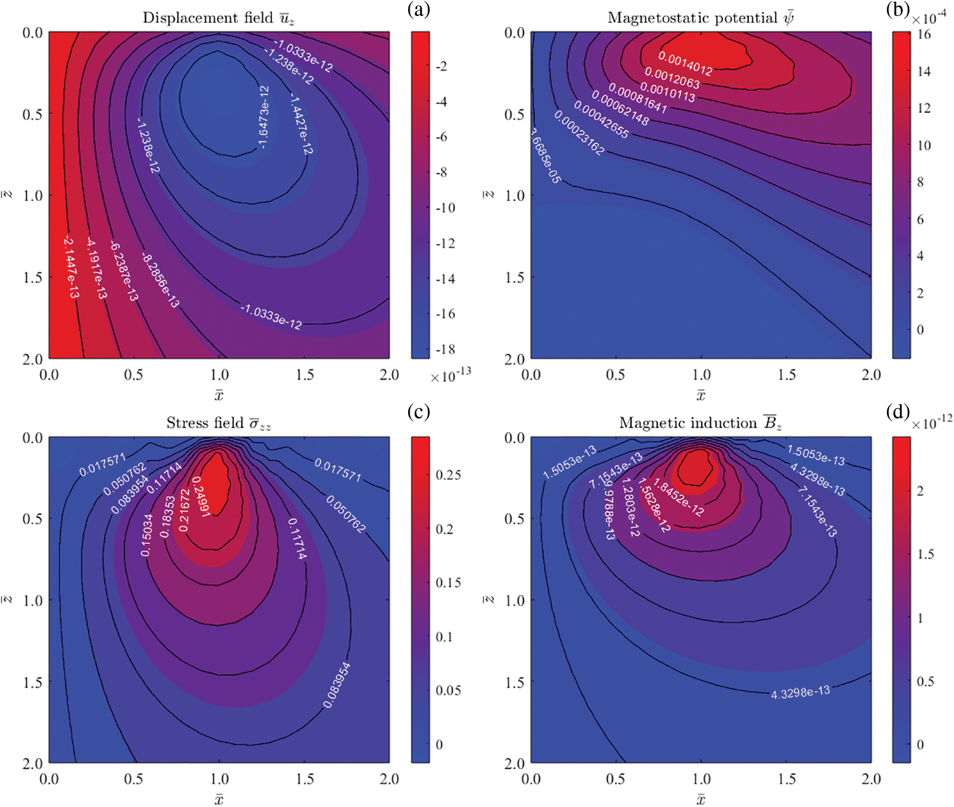
Figure 11: Contours of elastic displacement
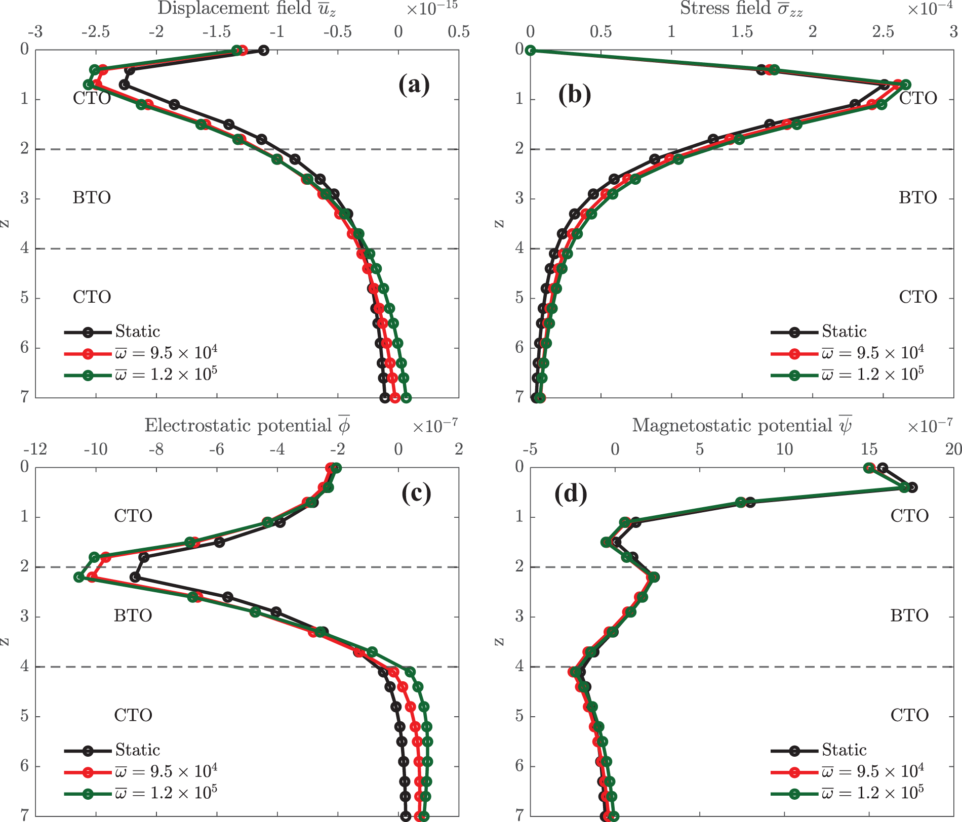
Figure 12: Effect of frequencies on elastic displacement
Fig. 11 presents 2D contours of elastic displacement
Fig. 12 presents the effect of different frequencies on elastic displacement
For a given multilayered MEE solid, we have derived the GFs due to surface (mechanical and electric) loads applied within a circle. The solution is in terms of the FBS along with the stable DVP matrix method for handling multiple layers. Since the involved coefficients are discrete Love numbers, we can pre-calculate, save, and repeatedly use them later on. Numerical examples are carried out for layered structures made of CoFe2O4 and BaTiO3, and the following features are observed:
1). Some physical quantities could be more sensitive to layering, while others not. For instance, under a vertical electric displacement on the surface, the electric potential is nearly independent of different layering structures, but other field quantities are completely different in different layering structures.
2). The primary physical quantities (displacements and electric/magnetic potentials) are more sensitive than others with frequency.
3). Field distributions in terms of contours are completely different under different (horizontal mechanical, vertical mechanical, and vertical electric) loads.
The results presented here provide valuable insights applicable across several domains. The contour plots illustrating elastic displacement, stress, electric potential, and magnetic potential under different mechanical and electric loads offer practical implications in advanced material science and engineering. Specifically, these findings are instrumental in the optimal design of different layered structures for enhancing mechanical and electromagnetic performance. Applications include the development of next-generation sensors capable of detecting subtle changes in stress and displacement, which are critical for structural health monitoring in civil infrastructure. In biomedical engineering, the ability to tailor material properties based on these findings supports the creation of biocompatible implants with improved durability and functionality. Moreover, in the realm of electromechanical systems, such as actuators and resonators, understanding frequency-dependent behaviors facilitates the design of more responsive and efficient devices for telecommunications and medical instrumentation.
While GFs lay out the significant insights and applications for the multilayered structure, there are limitations to this work that must be acknowledged. The key limitation of this work is the assumption of linear material behaviour, which may not accurately capture the complexities of real-world scenarios where nonlinear effects become significant. Future work should address this limitation by incorporating non-linearity into the material model.
Acknowledgement: The authors are grateful to the National Yang Ming Chiao Tung University, Taiwan, and Krishna Institute of Engineering and Technology, Ghaziabad, for providing all the essential research facilities.
Funding Statement: The National Science and Technology Council of Taiwan (Grant No. NSTC 111-2811-E- 516 A49-534) provided financial support for this study.
Author Contributions: Sonal Nirwal: Writing—original draft, Visualization, Validation, Methodology, Investigation, Formal analysis. Ernian Pan: Writing—review & editing, Supervision, Software, Project administration, Methodology, Funding acquisition, Conceptualization. Chih-Ping Lin: Writing—review & editing, Supervision, Project administration, Methodology, Funding acquisition. Quoc Kinh Tran: Writing—review & editing. All authors reviewed the results and approved the final version of the manuscript.
Availability of Data and Materials: All data analyzed during this study are included in this published article.
Ethics Approval: Not applicable.
Conflicts of Interest: The authors declare that they have no conflicts of interest to report in the present study.
References
1. Spaggiari A, Castagnetti D, Golinelli N, Dragoni E, Scirè MG. Smart materials: properties, design and mechatronic applications. Proc Inst Mech Eng L: J Mater Des Appl. 2019;233(4):734–62. doi:10.1177/1464420716673671. [Google Scholar] [CrossRef]
2. Barrett GR, Wolf N. High-rate, high-precision wing twist actuation for drone, missile, and munition flight control. Actuators. 2022;11(8):239. doi:10.3390/act11080239. [Google Scholar] [CrossRef]
3. Sharma S, Kiran R, Azad P, Vaish R. A review of piezoelectric energy harvesting tiles: available designs and future perspective. Energy Convers Manag. 2022;254:115272. doi:10.1016/j.enconman.2022.115272. [Google Scholar] [CrossRef]
4. Ganeson K, Tan XMC, Abdullah AAA, Ramakrishna S, Vigneswari S. Advantages and prospective implications of smart materials in tissue engineering: piezoelectric, shape memory, and hydrogels. Pharmaceutics. 2023;15(9):2356. doi:10.3390/pharmaceutics15092356. [Google Scholar] [PubMed] [CrossRef]
5. Suchtelen SJ. Product properties: a new application of composite materials. Philips Res Rep. 1972;27:28–37. [Google Scholar]
6. Eerenstein W, Mathur ND, Scott JF. Multiferroic and magnetoelectric materials. Nature. 2006;442(7104):759–65. [Google Scholar] [PubMed]
7. Nan CW, Bichurin MI, Dong S, Viehland D, Srinivasan G. Multiferroic magnetoelectric composites: historical perspective, status, and future directions. J Appl Phys. 2008;103(3):031101–35. [Google Scholar]
8. Vinyas M. Computational analysis of smart magneto-electro-elastic materials and structures: review and classification. Arch Comput Methods Eng. 2021;28(3):1205–48. [Google Scholar]
9. Berlincourt DA, Curran DR, Jaffe H. Piezoelectric and piezomagnetic materials and their function in transducers. Phys Acoust: Principles Methods. 1964;1:202–4. [Google Scholar]
10. Kopyl S, Surmenev R, Surmeneva M, Fetisov Y, Kholkin A. Magnetoelectric effect: principles and applications in biology and medicine–a review. Mater Today Bio. 2021;12:100149. [Google Scholar] [PubMed]
11. Liu H, Lyu Z. Modeling of novel nanoscale mass sensor made of smart FG magneto-electro-elastic nanofilm integrated with graphene layers. Thin-Walled Struct. 2020;151:106749. doi:10.1016/j.tws.2020.106749. [Google Scholar] [CrossRef]
12. Malleron K, Gensbittel A, Talleb H, Ren Z. Experimental study of magnetoelectric transducers for power supply of small biomedical devices. Microelectron J. 2019;88:184–9. doi:10.1016/j.mejo.2018.01.013. [Google Scholar] [CrossRef]
13. Li M, Liu M, Zhou L. The static behaviors study of magneto-electro-elastic materials under hygrothermal environment with multi-physical cell-based smoothed finite element method. Compos Sci Technol. 2020;193:108130. doi:10.1016/j.compscitech.2020.108130. [Google Scholar] [CrossRef]
14. Sasmal A, Arockiarajan A. Recent progress in flexible magnetoelectric composites and devices for next generation wearable electronics. Nano Energy. 2023;9:108733. doi:10.1016/j.nanoen.2023.108733. [Google Scholar] [CrossRef]
15. Rojas-Díaz R, Sáez A, García-Sánchez F, Zhang C. Time-harmonic Green’s functions for anisotropic magnetoelectroelasticity. Int J Solids Struct. 2008;45(1):144–58. doi:10.1016/j.ijsolstr.2007.07.024. [Google Scholar] [CrossRef]
16. Pan E. Green’s functions for geophysics: a review. Rep Prog Phys. 2019;82(10):106801. doi:10.1088/1361-6633/ab1877. [Google Scholar] [PubMed] [CrossRef]
17. Özdemir Ö., Yücel H, Uçar YE, Erbaş B, Ege N. Green’s functions for a layered high-contrast acoustic media. J Acoust Soc Am. 2022;151(6):3676–84. doi:10.1121/10.0011547. [Google Scholar] [PubMed] [CrossRef]
18. Buroni FC, Sáez A. Three-dimensional Green’s function and its derivative for materials with general anisotropic magneto-electro-elastic coupling. Proc R Soc A. 2010;466(2114):515–37. doi:10.1098/rspa.2009.0389. [Google Scholar] [CrossRef]
19. Hwu C, Chen WR, Lo TH. Green’s function of anisotropic elastic solids with piezoelectric or magneto-electro-elastic inclusions. Int J Fract. 2019;215:91–103. doi:10.1007/s10704-018-00338-6. [Google Scholar] [CrossRef]
20. Moshtagh E, Eskandari-Ghadi M, Pan E. Time-harmonic dislocations in a multilayered transversely isotropic magneto-electro-elastic half-space. J Intell Mater Syst Struct. 2019;30(13):1932–50. doi:10.1177/1045389X19849286. [Google Scholar] [CrossRef]
21. Yang ZX, Dang PF, Han QK, Jin ZH. Natural characteristics analysis of magneto-electro-elastic multilayered plate using analytical and finite element method. Compos Struct. 2018;185:411–20. doi:10.1016/j.compstruct.2017.11.031. [Google Scholar] [CrossRef]
22. Xiao D, Han Q, Jiang T. Guided wave propagation in a multilayered magneto-electro-elastic plate: theoretical analysis and numerical simulations. J Intell Mater Syst Struct. 2016;27(10):1295–309. [Google Scholar]
23. Vattré A, Pan E. Semicoherent heterophase interfaces with core-spreading dislocation structures in magneto-electro-elastic multilayers under external surface loads. J Mech Phys Solids. 2019;124:929–56. doi:10.1016/j.jmps.2018.11.016. [Google Scholar] [CrossRef]
24. Vattré A, Chiaruttini V. Singularity-free theory and adaptive finite element computations of arbitrarily-shaped dislocation loop dynamics in 3D heterogeneous material structures. J Mech Phys Solids. 2022;167:104954. doi:10.1016/j.jmps.2022.104954. [Google Scholar] [CrossRef]
25. Hung PT, Phung-Van P, Thai CH. Small scale thermal analysis of piezoelectric-piezomagnetic FG microplates using modified strain gradient theory. Int J Mech Mater Des. 2023;19(4):739–61. doi:10.1007/s10999-023-09651-y. [Google Scholar] [CrossRef]
26. Kiran MC. Thermal and hygrothermal buckling characteristics of porous magneto-electro-elastic skewed plates using third-order shear deformation theory. Mech Adv Mater Struct. 2023;1–16. doi:10.1080/15376494.2023.2227185. [Google Scholar] [CrossRef]
27. Lyu Z, Ma M. Nonlinear dynamic modeling of geometrically imperfect magneto-electro-elastic nanobeam made of functionally graded material. Thin-Walled Struct. 2023;191:111004. doi:10.1016/j.tws.2023.111004. [Google Scholar] [CrossRef]
28. Phung-Van P, Nguyen-Xuan H, Hung PT, Thai CH. Nonlinear isogeometric analysis of magneto-electro-elastic porous nanoplates. Appl Math Model. 2024;128:331–46. doi:10.1016/j.apm.2024.01.025. [Google Scholar] [CrossRef]
29. Zhao X, Li XY, Li YH. Axisymmetric analytical solutions for a heterogeneous multi-ferroic circular plate subjected to electric loading. Mech Adv Mater Struct. 2018;25(10):795–804. doi:10.1080/15376494.2017.1308586. [Google Scholar] [CrossRef]
30. Bui TQ, Hirose S, Zhang C, Rabczuk T, Wu CT, Saitoh T, et al. Extended isogeometric analysis for dynamic fracture in multiphase piezoelectric/piezomagnetic composites. Mech Mater. 2016;97:135–63. doi:10.1016/j.mechmat.2016.03.001. [Google Scholar] [CrossRef]
31. Kiran R, Nguyen-Thanh N, Yu H, Zhou K. Adaptive isogeometric analysis-based phase-field modeling of interfacial fracture in piezoelectric composites. Eng Fract Mech. 2023;288:109181. doi:10.1016/j.engfracmech.2023.109181. [Google Scholar] [CrossRef]
32. Manyo MJA, Ntamack GE, Azrar L. Time and frequency 3D-dynamic analyses of multilayered magnetoelectroelastic plates with imperfect interfaces. Arch Appl Mech. 2022;92(8):2273–301. doi:10.1007/s00419-022-02177-3. [Google Scholar] [CrossRef]
33. Vaezi M, Shirbani MM, Hajnayeb A. Free vibration analysis of magneto-electro-elastic microbeams subjected to magneto-electric loads. Phys E Low-Dimens Syst Nanostruct. 2016;75:280–6. doi:10.1016/j.physe.2015.09.019. [Google Scholar] [CrossRef]
34. Zhang XL, Chen XC, Yang E, Li HF, Liu JB, Li YH. Closed-form solutions for vibrations of a magneto-electro-elastic beam with variable cross section by means of Green’s functions. J Intell Mater Syst Struct. 2019;30(1):82–99. doi:10.1177/1045389X18803456. [Google Scholar] [CrossRef]
35. Zhao M, Zhang Q, Li X, Guo Y, Fan C, Lu C. An iterative approach for analysis of cracks with exact boundary conditions in finite magnetoelectroelastic solids. Smart Mater Struct. 2019;28(5):055025. doi:10.1088/1361-665X/ab0eb0. [Google Scholar] [CrossRef]
36. Liu M, Gan Q. Experimental research on dynamic response of layered medium under impact load. Coatings. 2022;12(10):1474. doi:10.3390/coatings12101474. [Google Scholar] [CrossRef]
37. Dong L, Closson AB, Jin C, Trase I, Chen Z, Zhang JX. Vibration-energy-harvesting system: transduction mechanisms, frequency tuning techniques, and biomechanical applications. Adv Mater Technol. 2019;4(10):1900177. doi:10.1002/admt.201900177. [Google Scholar] [PubMed] [CrossRef]
38. Pan E, Lin CP, Zhou J. Fundamental solution of general time-harmonic loading over a transversely isotropic, elastic and layered half-space: an efficient and accurate approach. Eng Anal Bound Elem. 2021;132:309–20. doi:10.1016/j.enganabound.2021.08.006. [Google Scholar] [CrossRef]
39. Love AEH. Some problems of geodynamics. Cambridge: Cambridge University Press; 1911. [Google Scholar]
40. Chu HJ, Zhang Y, Pan E, Han QK. Circular surface loading on a layered multiferroic half space. Smart Mater Struct. 2011;20(3):035020. doi:10.1088/0964-1726/20/3/035020. [Google Scholar] [CrossRef]
41. Zhou J, Pan E, Lin CP. A novel method for calculating dislocation Green’s functions and deformation in a transversely isotropic and layered elastic half-space. Eng Anal Bound Elem. 2023;152:22–44. doi:10.1016/j.enganabound.2023.03.022. [Google Scholar] [CrossRef]
42. Qi S, Zhang P, Ren J, Ma W, Wang J. Precise solutions of dynamic problems in stratified transversely isotropic piezoelectric materials. Arch Appl Mech. 2023;93(6):2351–88. doi:10.1007/s00419-023-02386-4. [Google Scholar] [CrossRef]
Cite This Article
 Copyright © 2024 The Author(s). Published by Tech Science Press.
This work is licensed under a Creative Commons Attribution 4.0 International License , which permits unrestricted use, distribution, and reproduction in any medium, provided the original work is properly cited.
 Downloads
 Citation Tools