A Fast and Memory-Efficient Direct Rendering Method for Polynomial-Based Implicit Surfaces

1  Introduction

Surface modeling from three-dimensional (3D) scattered points has many important applications including computer graphics, physics-based simulations, and medical imaging. A target object can be expressed by the implicit surface f(x)=0, where f(x) is a field comprising piecewise polynomials. Unlike the polygonal representation commonly employed in computer graphics, implicit surfaces are not always suitable for high-speed rendering because of their lack of explicit predefined surface geometry. Over the past few decades, various methods for generating implicit surfaces have been proposed, which can be roughly categorized into mathematical and machine learning approaches. Among the mathematical methods, one approach is to interpolate scattered surface points using radial basis functions (RBFs) [1–4]. The field is obtained as a linear combination of RFBs by solving a linear system of interpolating conditions. An alternative approach is to derive the signed distance function (SDF) for generating a field as a weighted sum of local fields [5,6]. Poisson surface reconstruction [7,8] involves creating a field based on the Poisson equation with hierarchical bases. Another approach is to approximate the field by using splines, from which piecewise polynomials can be extracted for fast rendering [9,10]. In particular, hierarchical B-splines [11] are efficient at representing a field on an adaptive grid. Recently, robust techniques have been proposed that can reconstruct surfaces from sparse and/or noisy point clouds [12]. Among machine learning methods, models are trained by using deep neural networks to express SDFs [13–16] or occupancy fields [17–20]. In particular, Huang et al. surveyed the current state of the art of machine learning methods [21].

Meanwhile, various methods have also been developed for visualizing implicit surfaces. A common strategy is polygonization or indirect rendering, which involves converting implicit surfaces to polygonal surfaces by using the marching cubes algorithm [22] or other advanced techniques [23,24]. Visualization is then performed by using standard polygonal rendering techniques. In contrast, direct rendering utilizes ray-casting to detect points on the original surface that correspond to screen pixels at the rendering stage. The simplest form of direct rendering is ray marching [25], which involves detecting the closest point on a surface corresponding to a single pixel by tracing a ray from the camera. More advanced direct rendering techniques such as sphere tracing [26] and adaptive marching points [27] help reduce the cost of finding intersections. In general, however, direct rendering suffers from high computational costs because surface points are searched iteratively for all screen pixels in every rendering frame. Thus, this approach is not suitable for fast rendering applications, especially when the field has a complicated expression.

In this paper, we propose a method for fast direct rendering of implicit surfaces that does not use intermediate polygonal representations. The proposed method comprises two main strategies: reducing the computational cost and narrowing the search range. For the first strategy, we employ piecewise polynomials [9,10] to represent the field of the implicit surface. For the second strategy, we limit the domain of the field to cells that intersect with the surface to exclude cells far from the surface. Fast rendering is achieved by designing the shader to exploit the structure of piecewise polynomials for efficient execution. The proposed method has several similarities with real-time ray casting [28], particularly in its capability for fast direct rendering of isosurfaces from discretely sampled fields such as volume data. This resemblance stems from the strategies of detecting cells intersecting the implicit surface and restricting the ray marching range to the detected cells. The proposed method is distinctive because it was designed for fields represented by piecewise polynomials. This design enables compatibility not only with standard grid cells but also with more general structures such as hierarchical B-splines.

2  Standard Rendering of Polynomial-Based Implicit Surfaces

2.1 Representing the Field of an Implicit Surface as Piecewise Polynomials

An implicit surface can be defined as f(x)=0, where x=(x,y,z) is an arbitrary point within the bounding box domain Ω and f(x) is the field. f(x) can be defined as a 3D uniform quadratic spline:

f(x)=∑i=−1Nx∑j=−1Ny∑k=−1Nzcijkbi(x)bj(y)bk(z)(x∈Ω),(1)

where bi(t) are the standard quadratic B-spline bases, cijk are the spline coefficients, and Nx, Ny, and Nz are the numbers of cells along x, y, and z axes, respectively. bi(t) are further defined as defined as:

bi(t)=b(t−i),

b(t)≡{(t+1)2/2(−1≤t<0)−t2+t+1/2(0≤t<1)(t−2)2/2(1≤t<2)0(otherwise).(2)

In this paper, we assume that the field is positive inside the implicit surface and negative outside the implicit surface. An arbitrary field defined in Ω can be approximated by the spline as defined in (1) using the technique described in [9]. The local field of a specific cell can then be expressed as a sixth-order polynomial:

fijk(x)=∑p=02∑q=02∑r=02αijk(p,q,r)xpyqzr(x∈Ωijk),(3)

when 0≤i≤Nx−1, 0≤j≤Ny−1, and 0≤k≤Nz−1, where Ωijk is the domain of the (i,j,k)-th local cell and αijk(p,q,r) represents the coefficient of the term xpyqzr. In other words, the local field can be expressed as a sixth-order polynomial with 27 terms, and it is defined independently from the other neighboring cells. Consequently, the number of polynomial coefficients to represent the field is 27NxNyNz in total. Fig. 1 shows an example of a polynomial-based field with 163 cells that is reconstructed from the point cloud of Stanford Bunny provided by the Stanford 3D Scanning Repository using the previously described technique [9]. The principal advantage of employing the polynomials is the simplicity of evaluating the field. Given a point x∈Ω, the cell corresponding to x can be easily identified by making use of the uniformity of the grid. Furthermore, the number of arithmetic operations required to evaluate the field remains constant regardless of the grid resolution.

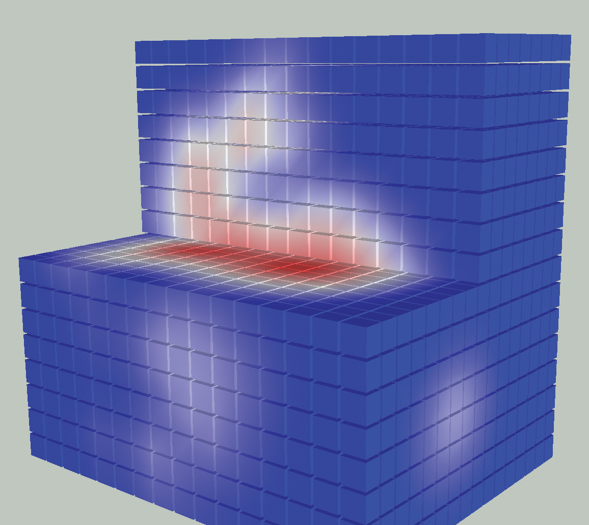
Figure 1: A polynomial-based field consisting of 163 local polynomials constructed from the Stanford Bunny point cloud using the grid of polynomials method [9]. The field is colored red and blue to indicate positive and negative values, respectively

2.2 The Ray Marching Algorithm

As shown in Fig. 2, ray marching renders the implicit surface f(x)=0, by tracing each ray until it intersects with the surface or exits the boundary of the domain. The tracing starts at the near-end of the domain x0, which is determined by the camera location c and position of the (i,j)-th screen pixel pij. Sampling is done at xk=x0+kΔdv, where v is the direction of the ray and Δd is the ray marching interval length. The interval length can be optimized to balance the tradeoff between rendering accuracy and processing speed. Although there is no obvious criterion for determining an appropriate interval length in general, a reasonable guideline is to select an interval length smaller than the cell size owing to the grid structure of the piecewise polynomials. The sampling continues until the ray crosses the implicit surface or reaches the far end of the domain. If k-th and (k+1)-th samples satisfy f(xk)<0 and f(xk+1)>0, respectively, an intersection is confirmed to exist within the interval between xk and xk+1. Thus, intervals with different signs at both ends can be detected, and the detection accuracy depends on the interval length. The intersection can be specified more accurately by applying the bisection method to the interval between xk and xk+1, which yields the final estimation of the intersection, xd. Finally, the pixel color is determined by the relation between the surface normal, the light source, and the material properties.

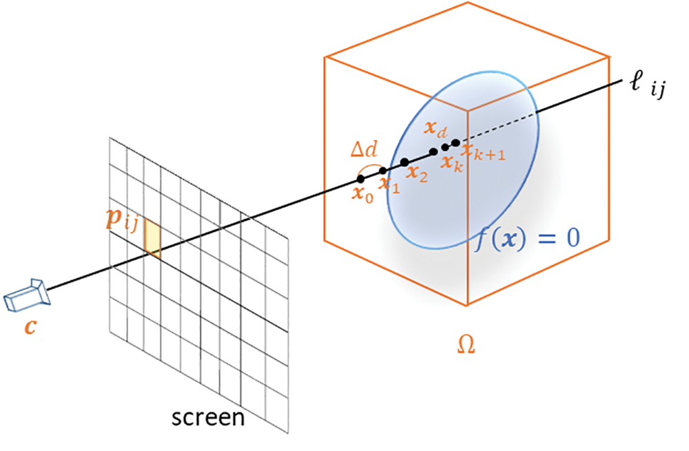
Figure 2: Conventional ray marching. If pij represents a screen pixel, then ray marching starts at the near end of the domain x0, and the ray is traced along the field at different sampling points until it intersects with the surface or the far end of the domain is reached

For fast rendering, the ray marching process should be parallelized on a graphics processing unit (GPU) shader. The conventional rendering method [9] is to parallelize the entire rendering process for a single frame, which is executed by a fragment shader of the GPU. If f(x) is defined within the bounding box Ω, this box is projected onto the screen for every frame, and the fragment shader is activated at all pixels within the projected area. Ray marching is then executed for each active fragment shader to determine the final color of each pixel. During this process, the cell index (i,j,k) of each sampling point should be identified to retrieve the 27 polynomial coefficients αijk(p,q,r) for evaluating the field at the (i,j,k)-th cell according to (3). If the coefficients of all cells are densely packed and stored in GPU memory, the cell index can be easily identified through a simple index operation [9]. However, the simple index operation is not feasible if the coefficients are stored sparsely, and an alternative approach is needed.

3  Proposed Method: Efficient Rendering for Polynomial Implicit Surfaces

The proposed method achieves fast direct rendering using piecewise polynomials and by limiting the ray marching range to around the surface. If the piecewise polynomials fijk(x) are given for all cells of the grid as detailed in Section 2.1, the range of ray marching and consequently the memory usage can be greatly reduced by limiting the cells to those that intersect with the surface. Fig. 3 illustrates the concept behind the method. The ray marching range is limited to cells intersecting the surface (i.e., active cells) by dividing the entire range into multiple segments based on cell boundaries and performing ray marching for every segment of the active cells. In the figure, a ray is segmented into three parts according to the active cells, and ray marching is performed at the three segments individually. Marching along a single ray provides not only the closest intersection but also other unnecessary intersections behind the closest intersection. Consequently, an additional process is needed to detect the closest intersection among all intersections after ray marching, for which we applied the standard depth test in OpenGL to the starting points of the segments. In the following subsections, we present the three main steps of the proposed method: identifying the active cells, developing a data structure for efficiently managing sparse active cells, and developing an algorithm for parallel execution on a GPU.

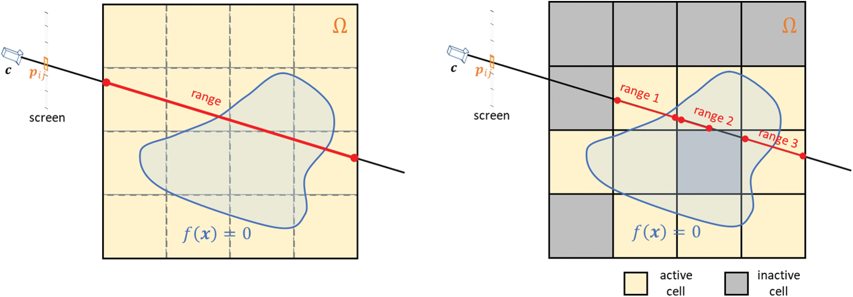
Figure 3: Example geometry for ray marching to render the implicit surface f(x)=0. The left side shows the conventional method [9], where the ray marching range is defined by the entire domain Ω. The right side shows the proposed method, where the ray marching range is defined by the active cells that intersect the ray, and ray marching is performed for each range segment with a starting point outside the surface

3.1 Identifying Active Cells

Active cells are identified by uniformly sampling each cell and evaluating the field. A cell is classified as active if its sampling points exhibit both positive and negative values and inactive otherwise. The sampling point density can be adjusted to balance the tradeoff between computational speed and accuracy. This process is performed during preprocessing, which is followed by sending the polynomial coefficients of the active cells to the GPU. Therefore, the time required for preprocessing is only needed once at the modeling and does not affect the subsequent actual rendering process. Fig. 4 summarizes rendering examples using different sampling resolution. The sampling density represents a trade-off between computational complexity and accuracy. In general, fine sampling is preferred in most cases because the time spent on preprocessing is required only during the modeling phase.

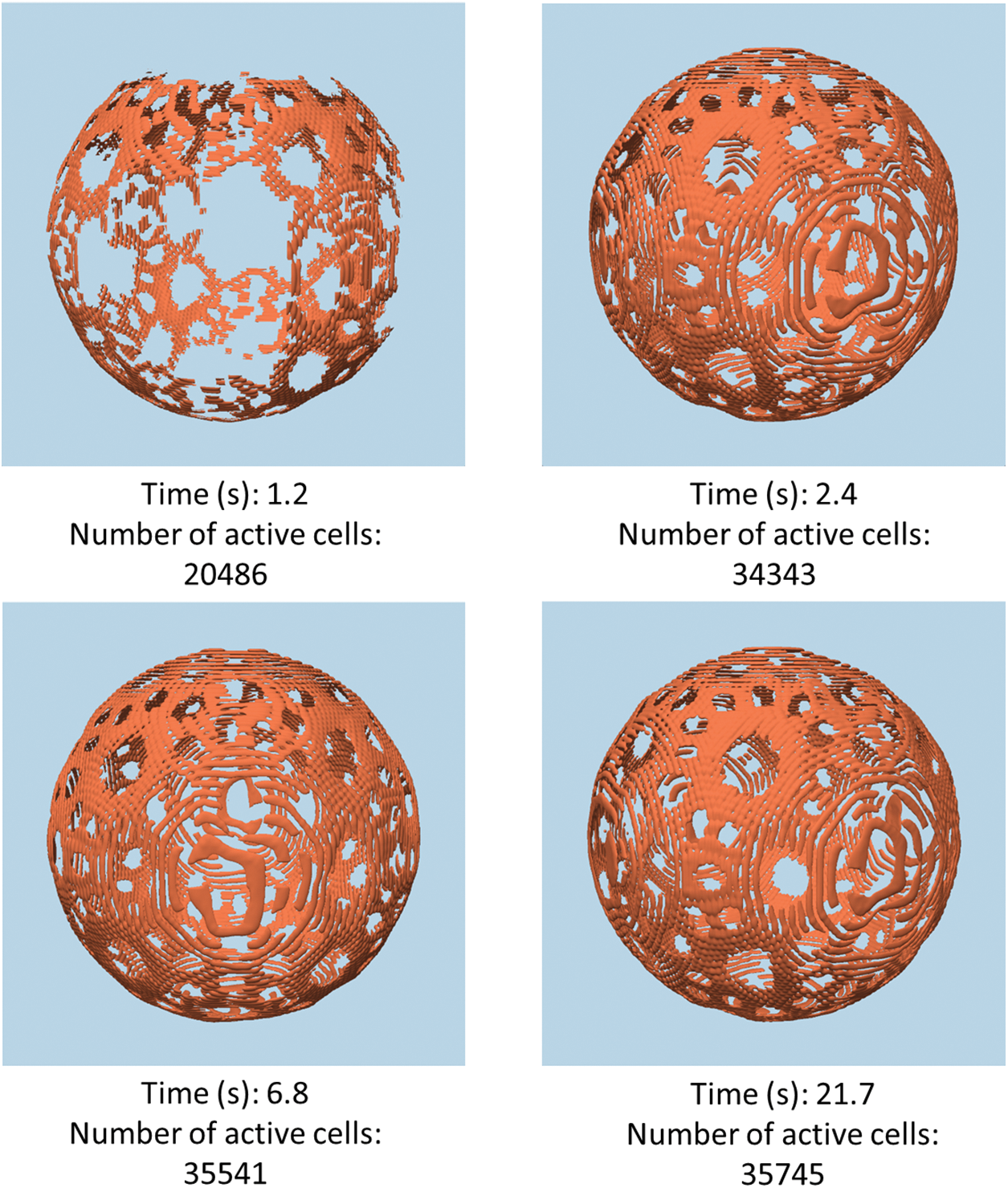
Figure 4: Rendering examples using different sampling resolutions for searching active cells. The resolution of the grid is 1283. The sampling resolution represents a trade-off between speed and accuracy

3.2 Efficient Data Structure

In the conventional method [9], piecewise polynomials are defined for all cells of the grid, and their coefficients are densely flattened into an array. For each sampling point xk along a ray, the cell index (i,j,k) corresponding to the sampling point is calculated. Then, the 27 coefficients αijk(p,q,r) corresponding to the current cell are retrieved from the flattened array, and the piecewise polynomial fijk(xk) is evaluated for the sign. The dense array benefits from a straightforward retrieval process because its layout reflects a regular grid structure, which allows coefficients to be located by using i, j, and k. However, the proposed method results in only a limited number of polynomial coefficients being stored, which makes accessing these coefficients more complex because the regular grid structure is not preserved. To realize an efficient data structure for accessing the sparsely stored polynomial coefficients, we introduce a supplementary mapping that correlates each cell index with its corresponding array index. Moreover, access to these coefficients can be optimized to GPU shaders. Fig. 5 illustrates the relation between active cells and the array of sparsely stored polynomial coefficients. In the proposed method, ray marching is performed within a single segment, which eliminates the need to access coefficients outside the targeted array segment.

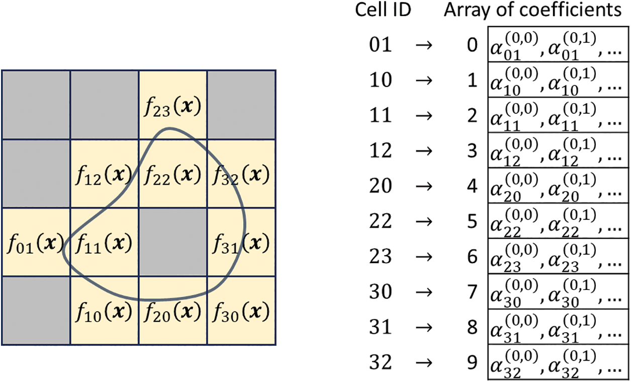
Figure 5: Two-dimensional example of extracting cells and the array of polynomial coefficients. The left side shows the extracted cells that intersect with f(x)=0. The right side shows the coefficients stored in an array after flattening and compression. Cell indices need to be mapped to array indices to allow the polynomial coefficients to be accessed

The ray marching process along a single ray segment is assigned to a fragment shader. The array of polynomial coefficients should satisfy the following two requirements:

•   A certain amount of memory space is required to store the polynomial coefficients of active cells in the GPU buffer, and each element of the array should be accessed efficiently from the fragment shader.

•   The fragment shader requires the current cell to be mapped to the array of polynomial coefficients stored on the GPU buffer.

For the first requirement, we send the array of polynomial coefficients to the GPU by using the shader storage buffer object (SSBO). Although other options are available such as the uniform buffer object (UBO) and vertex buffer object (VBO), the SSBO supports the sending of large arrays. Thus, the array can be sent to the SSBO prior to the rendering process and the elements can be accessed by the fragment shader. For the second requirement, we attach the index of the coefficient array to the attributes of all vertices and send the array index to the fragment shader so that it can access the polynomial coefficients at the current cell. Fig. 6 illustrates an example situation. Suppose that the polynomial coefficients of the (i,j,k)-th cell are stored at the IC-th element of the coefficient array and that each cell is composed of 12 triangles with 36 vertices, as shown on the right side. By adding the array index as an extra attribute, each of the 36 vertices now processes the attributes of the position, normal, and array index. The vertex shader receives the array index IC through the VBO, and the array index is sent from the vertex shader to the fragment shader as is. Thus, the fragment shader can access the polynomial coefficients at the current cell by using IC, which allows it to evaluate the piecewise polynomial fijk(x). Consequently, the sparse coefficient array αijk(p,q,r) comprising 27nactive floats is stored in the SSBO, and the vertex attributes (xl,yl,zl,nlx,nly,nlz,IC), comprising 7⋅36nactive floats in total is stored in the VBO, where nactive is the number of active cells. All components should be sent to the GPU only once before the render loop.

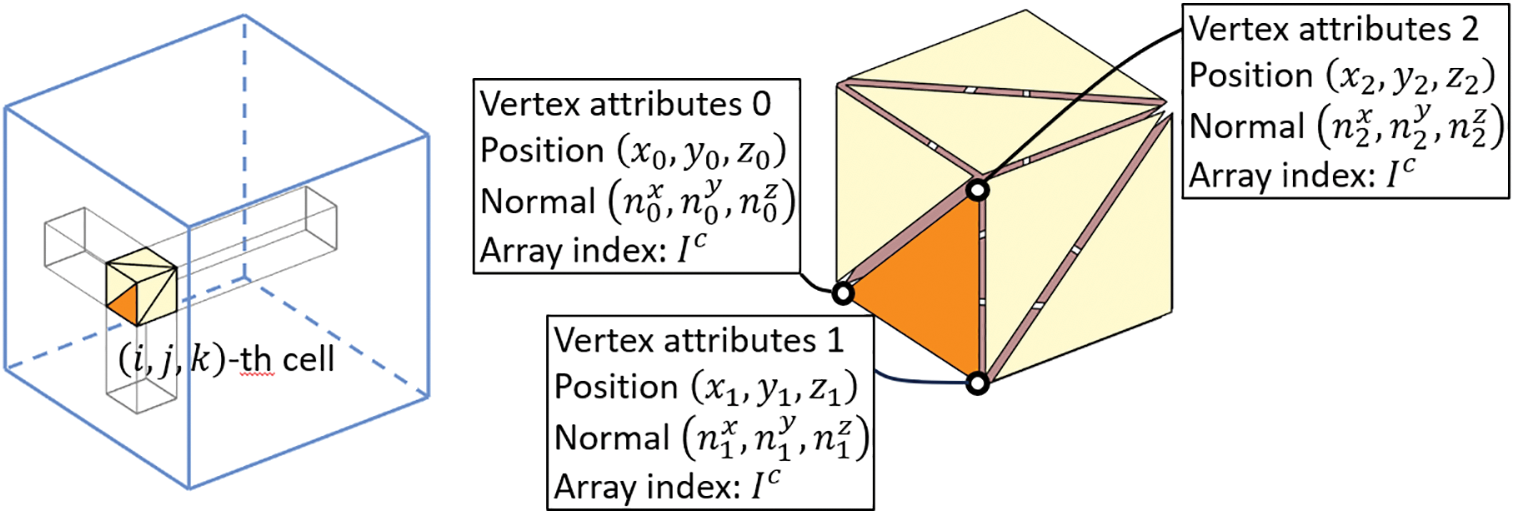
Figure 6: Example illustration of setting the attributes at each vertex of a cell. The coefficients of the (i,j,k)-th cell (left side) are stored at the IC-th element of the coefficient array, which is set as the array index at each vertex (right side)

3.3 Ray-Marching in Fragment Shader

The final ray marching is done in the render loop. Specifically, the 36nactive triangles comprising the active cells are projected onto the screen. Ray marching is executed if the projected triangle is facing forward, and it is discarded if the projected triangle is facing backward. This facilitates back-face culling and so that ray marching is executed for all fragments only on the front face. Ray marching at a single rasterized fragment requires the starting point x0, ray direction v, and polynomial coefficients αijk(p,q,r) at the cell. The starting point x0 is equivalent to the fragment position, and it is provided by default in the fragment shader owing to the projection of the triangles. The ray direction, v, can be derived from the camera and fragment positions. The polynomial coefficients αijk(p,q,r) can be retrieved from the array stored in the SSBO by using the index IC received from the vertex shader. Then, ray marching can be performed by repeatedly evaluating the local polynomial fijk(x) at the sampling points x0+kΔdv, where k=0,1,2…, until the sampling points cross the surface or exceed the current cell. One difference from the conventional ray marching is that a pixel can have multiple intersections, as shown in Fig. 7. In this case, the intersection closest to the screen should be selected, and the others should be discarded. To render only the closest point, we applied the standard depth test in OpenGL to the fragment positions. Although the depth at a fragment position is not that of an intersection, the depth test still works because the fragment positions are in the same order as the intersections.

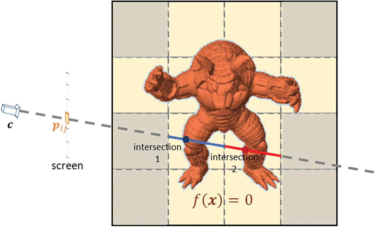
Figure 7: Example situation when a depth test is required. In this case, two intersections are found. Intersection 2 should be discarded, and intersection 1 should be used to determine the pixel color

4  Performance Evaluation

Experiments were performed to evaluate the rendering results of the proposed method compared with conventional ray marching. All experiments were performed by using a NVIDIA GeForce RTX 3090. The bisection method was fixed to 10 iterations, and the screen size was fixed to 1440 × 1440 pixels. Three example surfaces were used: Venus, Stanford Armadillo, and Holey Sphere. Venus is a relatively simple and smooth surface generated by a 3D scanning system [9], which should result in an accurate surface rendering even at a relatively low grid resolution. Stanford Armadillo was generated using the Stanford 3D Scanning Repository dataset, which has fine bumps on its surface. A Holey Sphere is an artificially generated spherical surface with holes. It has a very thin shape, so the grid resolution should be sufficient for accurate rendering. All implicit surfaces f(x)=0 were generated as a grid of piecewise polynomial method [9], and the local piecewise polynomials fijk(x)=0 was defined for each cell as given in (3). Three different grid resolutions were tested to examine the relationship between the accuracy and rendering speed: 323, 1283, and 5123. The ray-marching interval length Δd is another important factor that affects the accuracy and rendering speed. We define the interval length as Δd=diaΩ/M, where diaΩ is the diagonal of the entire domain and M is a user parameter that indicates the number of ray marching steps. Three values of M were tested corresponding to large (M=50), medium (M=500), and small (M=5000) interval lengths.

Figs. 8–10 show the rendering results of the proposed method. At M=50, the rendering resulted in missing portions of the surface and many pixels being shaded with the background color. This may be because the interval length was too large, and the ray marching skipped the limited active cells. This indicates that the proposed method requires a relatively small interval length to match the restricted ray marching range. Fig. 10 shows that a grid resolution of 323 was insufficient to accurately capture the thin shape. However, the rendering accuracy increased with M. These results indicate that the ray marching interval length should be adjusted depending on the fineness and thickness of the target object. In practice, accurate rendering was achieved with a sufficiently small ray marching interval length and sufficiently high grid resolution.

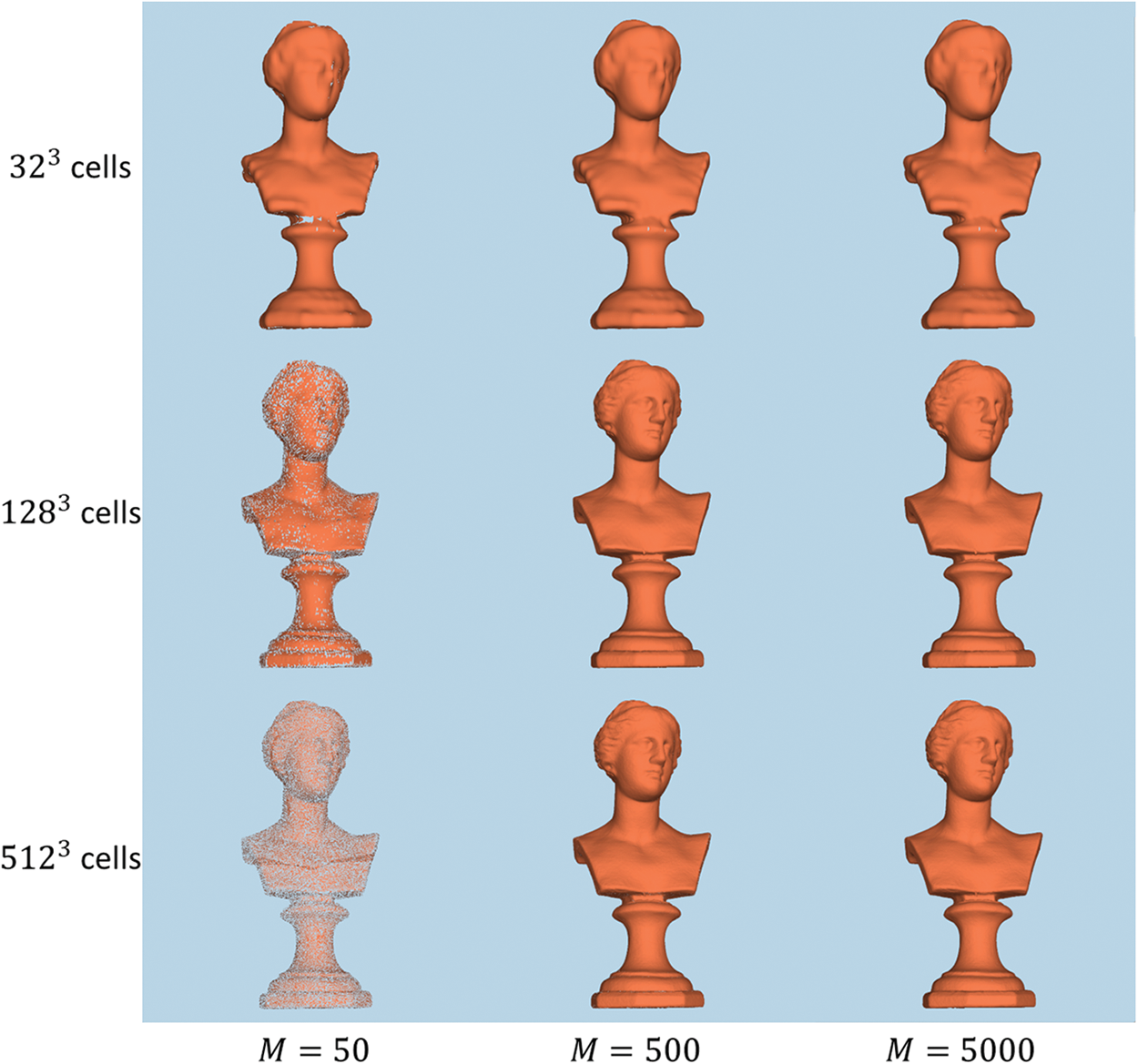
Figure 8: Rendering results for the shape Venus according to the grid resolution and interval length

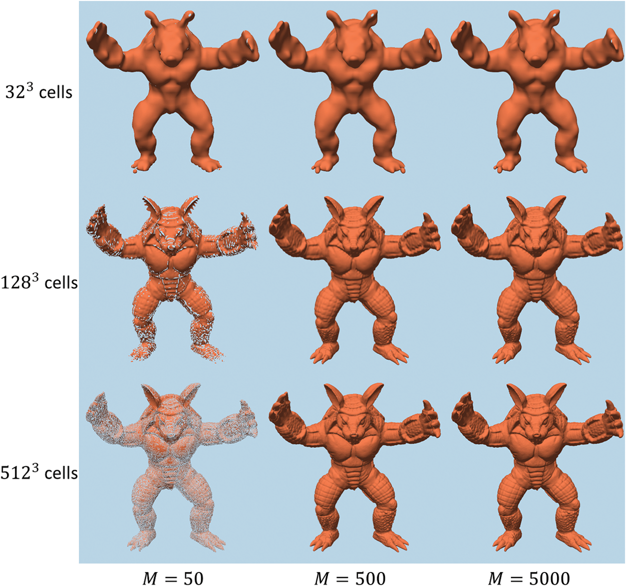
Figure 9: Rendering results for the shape Stanford Armadillo according to the grid resolution and interval length

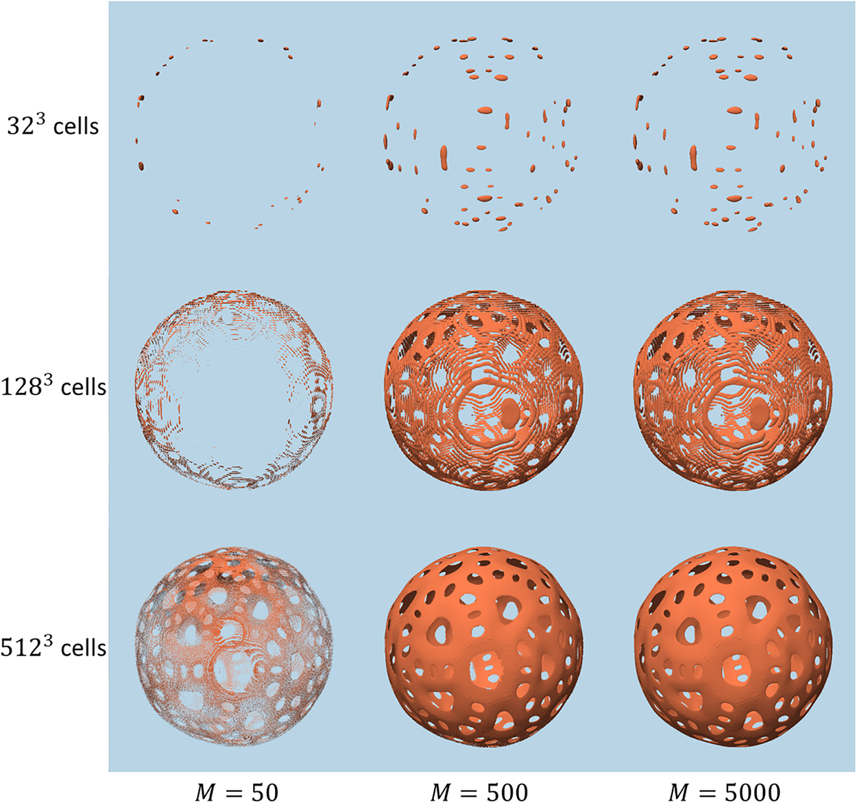
Figure 10: Rendering results for the shape Holey Sphere according to the grid resolution and interval length

Table 1 compares the rendering speeds of the proposed method and conventional ray marching in terms of the framerate (FPS). The proposed method demonstrated speedup factors of 1.1–218.2 in the test cases, which indicated that it was fast enough for real-time rendering even at high grid resolutions. The rendering speed of conventional ray marching for the grid resolution of 5123 cells was left blank because the memory usage exceeded the limits of the test environment.

Although many elements determine the speedup factor such as the distance from the bounding box to the surface and the projected area on the screen, a major factor is the ratio of active cells to the total number of cells. If the ratio is small, high computational efficiency can be expected because most of the sampling process in ray marching can be eliminated. Table 2 summarizes the number of active cells and their ratio to the total number of cells for each surface. A correlation was observed between the speedup factor and ratio. The GPU memory consumption can be derived from the number of active cells. For example, the maximum number of active cells in the experiments was about 1.1 million for the surface Holey Sphere at a grid resolution of 5123 cells. Considering that each cell has 27 polynomial coefficients, the SSBO required a total memory space of about 116 MB. Because each cell has 36 vertices, each with seven attributes (i.e., three coordinates, three normal components, and an index), the VBO requires a memory space of about 271 MB. These memory space requirements are manageable for typical GPUs, so the performance of the proposed method should be relatively independent of the computing environment. Thus, the proposed method is effective at reducing the ray marching range and memory consumption. These results confirm that the introduction of piecewise polynomials and restriction of the ray marching range greatly accelerated the direct rendering performance.

5  Conclusions and Future Work

Our proposed method accelerates the direct rendering of implicit surfaces by identifying active cells that intersect with the surface and performing ray marching in these cells rather than the whole domain, which greatly reduces the number of calculations compared to conventional ray marching. We developed a data structure specific to OpenGL shaders that uses both the SSBO and VBO. The fragment shader requires the polynomial coefficients for ray marching so the data structure was designed to allow efficient access of the coefficients by the fragment shader. The polynomial coefficients are stored in the SSBO and the index information that maps each cell to the corresponding coefficients is stored in the VBO. The experimental results showed that the proposed method achieved fast and direct rendering of various implicit surfaces. The results confirmed that the proposed method and data structure were effective, and reliable rendering results were obtained at a low computational cost when an appropriate ray marching interval length was selected. Moreover, we present a rendering procedure optimized for efficient execution on GPU shaders. The proposed method is specifically designed for polynomial-based implicit surfaces and is not applicable to general implicit surfaces unless they are converted to polynomial expressions with cubic cells. Although ray marching is a straightforward technique, it is expected to work effectively for finding intersections in each local cell. Additionally, this proposed method has the potential to be extended to a hierarchical cell structure using hierarchical B-splines in the future.

The proposed method limits ray marching to the vicinity of the implicit surface. Thus, its applicability is subject to certain limitations. For example, it cannot represent time-varying surfaces, which usually require polynomials over a larger range. Additionally, some operations that are characteristic of implicit surfaces, such as morphing and constructive solid geometry, require the full domain of the field, for which the proposed method is inapplicable. Future work will involve rendering implicit surfaces using piecewise polynomials representing not just the limited domain but also the entire domain. A possible solution would be to use an adaptive grid.

Acknowledgement: None.

Funding Statement: This work was supported by JSPS KAKENHI Grant Number 21K11928.

Author Contributions: The authors confirm contribution to the paper as follows: study conception and design: Jiayu Ren, Susumu Nakata; analysis and interpretation of results: Jiayu Ren, Susumu Nakata; draft manuscript preparation: Jiayu Ren; draft manuscript revision: Susumu Nakata. All authors reviewed the results and approved the final version of the manuscript.

Availability of Data and Materials: The data are available on request.

Ethics Approval: Not applicable.

Conflicts of Interest: The authors declare that they have no conflicts of interest to report regarding the present study.

References

1. Carr JC, Beatson RK, Cherrie JB, Mitchell TJ, Fright WR, McCallum BC, et al. Reconstruction and representation of 3D objects with radial basis functions. In: Proceedings of the 28th Annual Conference on Computer Graphics and Interactive Techniques. SIGGRAPH ’01, 2001; New York, NY, USA: Association for Computing Machinery; p. 67–76. [Google Scholar]

2. Turk G, O’Brien JF. Modelling with implicit surfaces that interpolate. ACM Trans Graph. 2002;21(4): 855–73. doi:10.1145/571647.571650. [Google Scholar] [CrossRef]

3. Morse BS, Yoo TS, Rheingans P, Chen DT, Subramanian KR. Interpolating implicit surfaces from scattered surface data using compactly supported radial basis functions. In: Proceedings of the International Conference on Shape Modeling and Applications, 2001; Genova, Italy: IEEE Computer Society; p. 89–98. doi:10.1109/SMA.2001.923379. [Google Scholar] [CrossRef]

4. Zeng Y, Zhu Y. Implicit surface reconstruction based on a new interpolation/approximation radial basis function. Comput Aided Geom Des. 2022;92(4):102062. doi:10.1016/j.cagd.2021.102062. [Google Scholar] [CrossRef]

5. Ohtake Y, Belyaev A, Alexa M, Turk G, Seidel HP. Multi-level partition of unity implicits. ACM Trans Graph. 2003;22(3):463–70. doi:10.1145/882262.882293. [Google Scholar] [CrossRef]

6. Tobor I, Reuter P, Schlick C. Reconstructing multi-scale variational partition of unity implicit surfaces with attributes. Graph Models. 2006;68(1):25–41. doi:10.1016/j.gmod.2005.09.003. [Google Scholar] [CrossRef]

7. Kazhdan M, Bolitho M, Hoppe H. Poisson surface reconstruction. In: Proceedings of the Fourth Eurographics Symposium on Geometry Processing, 2006; Cagliari, Sardinia, Italy: Eurographics Association; vol. 7 no. 4, p. 61–70. [Google Scholar]

8. Manson J, Petrova G, Schaefer S. Streaming surface reconstruction using wavelets. Comput Graph Forum. 2008;27:1411–20. [Google Scholar]

9. Nakata S, Aoyama S, Makino R, Hasegawa K, Tanaka S. Real-time isosurface rendering of smooth fields. J Vis. 2012;15(2):179–87. doi:10.1007/s12650-011-0119-5. [Google Scholar] [CrossRef]

10. Itoh T, Nakata S. Fast generation of smooth implicit surface based on piecewise polynomial. Comput Model Eng & Sci. 2015;107(3):187–99. doi:10.3970/cmes.2015.107.187. [Google Scholar] [CrossRef]

11. Pan M, Tong W, Chen F. Phase-field guided surface reconstruction based on implicit hierarchical B-splines. Comput Aided Geom Des. 2017;52–53(6):154–69. doi:10.1016/j.cagd.2017.03.009. [Google Scholar] [CrossRef]

12. Liu XY, Wang H, Chen CS, Wang Q, Zhou X, Wang Y. Implicit surface reconstruction with radial basis functions via PDEs. Eng Anal Bound Elem. 2020;110(4–5):95–103. doi:10.1016/j.enganabound.2019.09.021. [Google Scholar] [CrossRef]

13. Erler P, Guerrero P, Ohrhallinger S, Mitra NJ, Wimmer M. POINTS2SURF learning implicit surfaces from point clouds. arXiv:2007104532020. 2020. [Google Scholar]

14. Liu SL, Guo HX, Pan H, Wang PS, Tong X, Liu Y. Deep implicit moving least-squares functions for 3D reconstruction. arXiv:2103122662021. 2021. [Google Scholar]

15. Ma B, Han Z, Liu YS, Zwicker M. Neural-pull: learning signed distance functions from point clouds by learning to pull space onto surfaces. arXiv:2011134952021. 2021. [Google Scholar]

16. Ma B, Liu YS, Han Z. Reconstructing surfaces for sparse point clouds with on-surface priors. arXiv:2204106032022. 2022. [Google Scholar]

17. Jia M, Kyan MJ. Learning occupancy function from point clouds for surface reconstruction. arXiv:2010113782020. 2020. [Google Scholar]

18. Peng S, Niemeyer M, Mescheder L, Pollefeys M, Geiger A. Convolutional occupancy networks. arXiv:2003046182020. 2020. [Google Scholar]

19. Martel JN, Lindell DB, Lin CZ, Chan ER, Monteiro M, Wetzstein G. ACORN: adaptive coordinate networks for neural scene representation. arXiv:2105027882021. 2021. [Google Scholar]

20. Takikawa T, Litalien J, Yin K, Kreis K, Loop C, Nowrouzezahrai D, et al. Neural geometric level of detail: real-time rendering with implicit 3D shapes. arXiv:2101109942021. 2021. [Google Scholar]

21. Huang Z, Wen Y, Wang Z, Ren J, Jia K. Surface reconstruction from point clouds: a survey and a benchmark. arXiv:2205024132022. 2022. [Google Scholar]

22. Newman TS, Yi H. A survey of the marching cubes algorithm. Comput Graph. 2006;30(5):854–79. doi:10.1016/j.cag.2006.07.021. [Google Scholar] [CrossRef]

23. Stander BT, Hart JC. Guaranteeing the topology of an implicit surface polygonization for interactive modeling. In: Proceedings of the 24th Annual Conference on Computer Graphics and Interactive Techniques. SIGGRAPH ’97, 1997; USA: ACM Press/Addison-Wesley Publishing Co.; p. 279–86. [Google Scholar]

24. Gelas A, Valette S, Prost R, Nowinski WL. Variational implicit surface meshing. Comput Graph. 2009;33(3):312–20. [Google Scholar]

25. Perlin K, Hoffert EM. Hypertexture. ACM SIGGRAPH Comput Graph. 1989;23(3):253–62. [Google Scholar]

26. Hart JC. Sphere tracing: a geometric method for the antialiased ray tracing of implicit surfaces. Vis Comput. 1996;12(10):527–45. [Google Scholar]

27. Singh JM, Narayanan PJ. Real-time ray tracing of implicit surfaces on the GPU. IEEE Trans Vis & Comput Graph. 2010;16(2):261–72. [Google Scholar]

28. Hadwiger M, Sigg C, Scharsach H, Bühler K, Gross MH. Real-time ray-casting and advanced shading of discrete isosurfaces. Comput Graph Forum. 2005;24(3):303–12. [Google Scholar]