Concurrent Two–Scale Topology Optimization of Thermoelastic Structures Using a M–VCUT Level Set Based Model of Microstructures

1  Introduction

A thermoelastic structure in this study is subjected to both temperature changes and mechanical forces. Optimization of thermoelastic structures with the aim of compliance minimization leads to some unusual and interesting results, as discussed in our previous study [1], and this motivated the present work of concurrent two-scale topology optimization. When the classical Solid Isotropic Microstructure with Penalization (SIMP) method is applied to solve the thermoelastic problem, many “gray” densities persist in the optimized structures even when the penalty parameter is increased, as shown in Fig. 1. In fact, such a structure with “gray” densities is indeed better than a “black–white” structure for this optimization problem [1]. More importantly, recalling that the “gray” densities in the SIMP method represent isotropic microstructures, we see that introducing microstructures into the topology optimization of thermoelastic structures will have great significance.

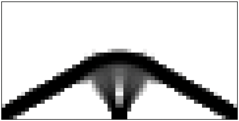
Figure 1: The optimized thermoelastic structure based on SIMP method, where gray densities imply isotropic microstructures

According to the observation mentioned above, one can see that it would be better if the optimization of thermoelastic structures was solved in both the macro scale and the microscale so that different microstructures can be properly distributed in the structure to match different requirements at different positions and directions.

Two-scale topology optimization has caught much attention in the past decades, and many methods were proposed [2,3]. One important category of methods is based on the optimal microstructure prototype known a priori for the optimization problem or those specified by designer [4–7]. For example, in the minimum compliance problem under a single load, laminate microstructures have been rigorously shown to be optimal [8,9], and specified lattice structures are applied in two–scale optimization [10–13]. During the optimization, some parameters that describe the shape or topology of microstructures are iteratively updated, and different microstructures appear. In addition, based on this method, people also proposed to post-process the result to obtain a structure on a fine grid in the macro scale [14–18]. However, in this category of methods, the diversity of shape and topology of the optimized microstructure is not so rich.

The other category, often referred to as hierarchical or concurrent methods [19–23], does not require microstructural prototypes and allows microstructures at different locations of the structure to generate different configurations freely. This approach is more flexible, but the issue of connectivity between neighboring microstructures arises. Many efforts were made to address the connectivity issue [24–28].

Based on these previous research works, it is clear that the microstructure model has important impacts on two-scale topology optimization. Given this, an alternative microstructure model is proposed in the present study. The geometry of microstructure is described by the multiple variable cutting (M–VCUT) level set method proposed in our previous studies [29,30]. A microstructure is obtained by combining multiple virtual microstructures that are derived respectively from multiple microstructure prototypes. Then, the microstructures are treated as homogeneous materials in the macro scale, and their effective mechanical properties are dealt with respectively by two different approaches in an offline phase and an online phase. In the offline phase, the effective properties are computed by homogenization. Then, a mapping relationship between effective properties and design variables is established, which gives a data-driven model of microstructure. In the online phase, i.e., during the optimization, the data-driven model is used.

In our previous studies on the optimization of cellular structures [29,30], full-scale finite element analysis (FEA) with a fine mesh of elements was used, and this induces high computational costs. To improve the efficiency of the FEA, a data-driven model is employed. The benefits are two-fold. First, by deriving microstructures from multiple microstructure prototypes, the layouts of microstructures become more diverse, thus providing more flexibility for design optimization, and at the same time the connectivity between microstructures is ensured. Second, because the computational costs of using such a data-driven model are much less than those of homogenization, the efficiency of FEA is improved.

2  Geometry Model and Homogenization of Microstructure

2.1 Geometry Model of Microstructure

A two–scale structure Ω⊂Rd (d=2 or 3) is optimized within a fixed reference domain D⊂Rd, and the domain is decomposed into cells Dk (k=1...M), i.e., D=∪k=1MDk. In each cell Dk, there may exist a microstructure Ωk, i.e., Ωk⊂Dk. Similarly, a two–scale structure Ω is given by

Ω=∪k=1MΩk(1)

The microstructures Ωk are described by using the M–VCUT level set method [29,30]. Each Ωk is described by using multiple basic level set functions Φik (i=1...N) and multiple cutting functions Ψik (i=1...N). Each Φik represents a microstructure prototype and remains unchanged during the optimization. The cutting function is a horizontal plane with a constant height hik here, i.e.,

Ψik(x)=hik, ∀x∈Dk(2)

The function Υik is used to represent the result of a cutting operation between Φik and Ψik, i.e.,

Υik(x)=Φik(x)−hik, x∈Dk, k=1…M, i=1…N(3)

After all the cutting operations are finished in Dk, N virtual microstructures Ω~ik defined by the function Υik are obtained as

Ω~ik={x|Υik (x)<0, x∈Dk}(4)

Examples of the cutting operation are shown in Fig. 2.

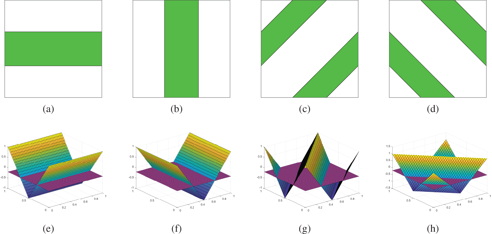
Figure 2: Description of the cutting operation. (a)–(d) four virtual microstructures obtained by the cutting operation, (e)–(h) four basic level set functions with the cutting planes shown in purple color

With all the virtual microstructures in Dk, one obtains an actual microstructures Ωk by combining them together, i.e.,

Ωk=∪i=1NΩ~ik(5)

The combination operation in Eq. (5) can be realized by

Υk(x)=min{Υ1k(x),…,ΥNk(x)}(6)

where Υk is the function used to define the actual microstructure Ωk, i.e.,

Ωk={x|Υk(x)<0, x∈Dk}(7)

With the basic level setting function shown in Fig. 2, various actual microstructures can be obtained by changing the height of the cutting plane, as shown in Fig. 3.

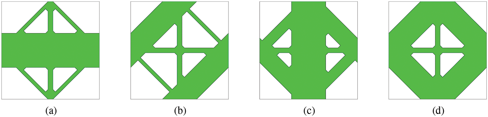
Figure 3: Actual microstructures generated based on the basic level set functions shown in Fig. 2. The heights of cutting planes for each microstructure are as follows: (a) h1=−0.2, h2=−0.8, h3=−0.8, h4=−0.8; (b) h1=−0.8, h2=−0.8, h3=−0.2, h4=−0.8; (c) h1=−0.8, h2=−0.2, h3=−0.6, h4=−0.4; (d) h1=−0.8, h2−0.8, h3=−0.2, h4=−0.2

It should be noted that although the examples shown in Figs. 2 and 3 are obtained from the four microstructure prototypes, the number and type of prototypes are unrestricted in this method, and the prototypes can be modified according to different requirements.

In the optimization process, the only parameter of the cutting plane Ψik is the height hik, which is the design variable, and all the heights hik are changed according to the optimization algorithm, thus changing the virtual microstructure Ω~ik, and then the actual microstructure Ωk, and finally the double-scale structure Ω.

In the optimization, the design variables are the heights hik of cutting planes. They are changed according to an optimization algorithm, thus changing the virtual microstructure Ω~ik, then the actual microstructures Ωk, and in the end the two-scale structure Ω.

2.2 Homogenization of Microstructure

In the two-scale optimization, the effective mechanical properties of microstructures are an important link between the macroscale and microscale. The homogenization method [4,31] is applied in an offline phase to compute the effective mechanical properties of the unit cells:

EijklH=1|Y|∫YEpqrs(εpq0(ij)−εpq(ij))(εrs0(kl) −εrskl)dY(8)

where Epqrs is the elastic tensor of the material of the microstructure; |Y | is the volume of the cell; εpq0(ij) is the prescribed strain in macroscale; εpq(ij) denotes the strain in microscale defined as

εpq(ij)=εpq(χij)=12(χp, qij+χq, pij)(9)

where χij is obtained by solving the equation

∫YEijpqεij(v)εpq(χkl)dY=∫YEijpqεij(v)εpq0(χkl)dY, ∀v∈V(10)

where v is the virtual displacement. For 2D problems, the results are rewritten in a matrix form as

DH=[D11HD12HD13HD21HD22HD23HD31HD32HD33H],DmnH=DnmH(11)

3  Mapping Relationship between hi and DH

Although numerical homogenization is a powerful tool for obtaining the effective elastic modulus of a microstructure, it leads to high computational costs for two–scale structures containing many microstructures. The costs are more prominent in the optimization that usually needs tens or hundreds of iterations. Therefore, in this paper, numerical homogenization is only done in an offline phase to generate data samples. Thereafter, these data samples are used to construct a simple numerical mapping model between the effective elastic modulus DH and the design variables hi. In the end, such a mapping model is used in the online optimization phase, more specifically in the macroscale FEA and sensitivity analysis. Because the computational costs of invoking such a mapping model are much less than those of homogenization, the efficiency of analysis and optimization of two-scale structures is improved. Such a mapping model can be regarded as a generalized model of anisotropic material microstructure whose role in structural optimization is similar to that of the power law model of the SIMP method.

3.1 Database of Microstructures

To establish the mapping relationship, we need a database that contains many data samples. The process of database creation is described below.

The range of all the basic level set functions Φi is [−1, 1], as shown in Fig. 2. In addition, to ensure that empty microstructure and full microstructure can be obtained, the ranges of the cutting heights hi are enlarged to [−1.2, 1.2]. Then, the cutting heights hi are uniformly sampled in this interval with a spacing of 0.1. In other words, we have four microstructure prototypes, and we generate 25 virtual microstructures by changing the cutting height of each microstructure prototype with a spacing of 0.1. According to our numerical experience, such spacing is a proper compromise between the size of the database and the accuracy of the mapping relationship.

For each combination of the cutting heights hi, we generate an actual microstructure and then create a data sample in the database. Therefore, if four microstructure prototypes are used, a total of 254 data samples are created in the database. Each data sample includes all the information required by the two-scale optimization, i.e., the cutting heights hi, the elastic modulus DH, and the volume VH of the microstructure sample. Here, the VH is obtained by numerical integration of the region occupied by the microstructure sample.

3.2 Radial Basis Function (RBF) Based Interpolation

With the database of microstructure, many methods can be used to construct the mapping relationship, for instance, the linear or low-order polynomials interpolation, neural networks, or surrogate models. In this paper, the RBF interpolation is used [32,33], because of its unique solvability, smoothness, and accuracy [34–38].

The Compact Support Radial Basis Function (CS–RBF) [32] is used to construct a local interpolation function by using a small amount of data around the evaluation point (denoted h). Here, h is a column vector whose components are the cutting heights, i.e., h=[h1,…,hN]T and N is the number of cutting planes. The computational costs of such local interpolation are much lower than that of homogenization.

Using the CS–RBF interpolation, the elastic matrix DH and the volume VH of an actual microstructure with the cutting heights h can be obtained as

DmnH(h)=∑q=1Qαqmnϕ(rq(h))(12)

VH(h)=∑q=1Qβqϕ(rq(h))(13)

where αqmn and βq are the coefficients of the CS–RBFs; Q denotes the required number of data samples for local interpolation; rq is a function of h defined as

rq(h)=1ds||h−h^q||2+σ2(14)

where h^q=[h^1,…,h^N]T are the data points stored in the database; ||h−h^q|| is the Euclidean distance between h and h^q; ds is the support radius, and it is set to 2; σ is a positive number set to 0.05. For better interpolation, the CS–RBF with C2 continuity is chosen, as shown in Eq. (15).

ϕ(rq)=max{0, (1−rq)4}(4rq+1)(15)

The coefficients αqmn and βq of the CS–RBFs are obtained by solving equations that enforce values of interpolation functions that agree with data samples in the database. Such a system of linear equation of αqmn is given by

DmnH(h^q)=[D^mnH]q,q=1,…,Q(16)

where h^q is the cutting height vector of the q-th data sample in the local region of interpolation; [D^mnH]q is the effective elastic modulus related to h^q. Here, h^q and [D^mnH]q are stored in the database. The matrix form of Eq. (16) is written as

[ϕ1,1…ϕ1,Q⋮⋱⋮ϕQ,1…ϕQ,Q][α1mn⋮αQmn]=[[D^mnH]1⋮[D^mnH]Q](17)

where ϕi,j is given by

ϕi, j=ϕ(1ds||h^i−h^j||2+σ2),i, j=1…Q(18)

Based on the four microstructures in Section 2.1, a mapping relationship between the design variables to the effective elasticity matrix of the microstructures is established. For example, when the design variable h=[−0.42, −0.87, −0.68, −0.35]T, the virtual microstructures are shown in Fig. 4a–d, and the actual microstructure is shown in Fig. 4e. The elastic matrix of the actual microstructure can be obtained by the RBF interpolation, and the result is

DH=[0.52540.1539−0.02650.15390.4404−0.0235−0.0265−0.02350.1615](19)

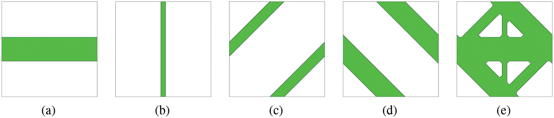
Figure 4: Example of mapping relationship from design variables to microstructures: (a)–(d) four virtual microstructures, (e) actual microstructure

4  Optimization Problem of Two–Scale Thermoelastic Structures

The two–scale optimization of thermoelastic structures was investigated in many previous studies [39–41]. The optimization problems include multi-obiective problem [42], multi-material problem [43], and uncertainty problem [44]. In this paper, the compliance minimization of two-scale thermoelastic structures subjected to a uniform temperature change is considered.

minC=f1Tu+f2Tu  s.t.Ku=f1+f2hmin≤hik≤hmaxV−V¯≤0(20)

where C is the compliance; f1 and f2 are the global thermal and global mechanical load vectors, respectively; K is the global stiffness matrix; u is the global displacement vector; hmin and hmax are respectively the upper and lower bounds of the design variable hik; V is the volume of the two–scale structure, with V¯ as the upper bound.

The global stiffness matrix K is written as

K=∑e=1M∫ΩeBTDeHBdx(21)

where Ωe is the e-th element; DeH denotes effective elastic modulus for the e-th element, and it is obtained by the CS–RBF interpolation; B is the strain-displacement matrix. In this study, each cell Dk is treated as a finite element in the macro-scale FEA.

The global thermal load vector f1 is given by

f1=∑e=1M∫ΩeBTDeHεtdx(22)

where the thermal strain εt in plance stress state is given by

εt=αΔTδ(23)

where α is the coefficient of thermal expansion of the material; ν is the Poisson’s ratio; δ is the unit tensor, which is [1 1 0]T in the planar problem; and ΔT denotes temperature change. The temperature change ΔT is assumed to be uniform. Note that α is independent of the microstructure composed of one material [45].

5  Sensitivity Analysis

To calculate the derivative of C concerning hik, the objective function is rewritten by adding the state equation as a constraint

C=f1Tu+f2Tu−u~T(Ku−f1−f2)(24)

where u~ is the Lagrange multiplier, also known as the adjoint vector. Then, the derivative is

∂C∂hik=(uT+u~T)∂f1∂hik−u~T∂K∂hiku+(f1T+f2T−u~TK)∂u∂hik(25)

Because u does not have an explicit relationship to the design variable hik, calculation of ∂u∂hik should be avoided. Therefore, the coefficient of this derivative is set to zero.

f1T+f2T−u~TK=0(26)

Comparing Eq. (26) with the state equation in the optimization problem Eq. (20), we get

u~=u(27)

Applying the Eq. (27), we can simplify Eq. (25), so that the derivatives is

∂C∂hik=2uT∂f1∂hik−uT∂K∂hiku(28)

Then, substituting Eqs. (21) and (22) into (28), we get

∂C∂hik=2ueT∫ΩeBT∂DeH∂hikεtdx−ueT(∫ΩeBT∂DeH∂hikBdx)ue(29)

where ue is the displacement vector.

The derivative of the elastic matrix DeH with respect to hik in 2D problems is

∂DeH∂hik=[∂[D11H]e∂hik∂[D12H]e∂hik∂[D13H]e∂hik∂[D21H]e∂hik∂[D22H]e∂hik∂[D23H]e∂hik∂[D31H]e∂hik∂[D32H]e∂hik∂[D33H]e∂hik](30)

According to the interpolation function in Eq. (12), we have

∂[DmnH]e∂hik=∑q=1Qαqmn∂ϕ(rq)∂hik(31)

According to the definition of CS–RBF in Eq. (15), we have

∂ϕ(rq)∂hik=∂ϕ∂rq∂rq∂hik=max{0, (1−rq)3}(−20rq)∂rq∂hik(32)

Finally, according to Eq. (14), we have

∂rq∂hik=hik−h^q, ids||h−h^q||2+σ2(33)

The volume in the constraint function is the sum of the volumes of all the elements, which are also obtained from the mapping relationship. Therefore, the sensitivity analysis of the volume constraint function can also be performed by the above method. In this study, the Method of Moving Asymptotes (MMA) algorithm is used for optimization [46].

6  Numerical Example

Several examples of two–scale thermoelastic structural optimization are presented. Relevant properties of the material used in these examples are as follows: coefficient of thermal expansion α=15.4×10−3(/K), Young’s modulus E=1(Pa), and Poisson’s ratio ν=0.3. To avoid singularities in FEA, an artificially weak material is defined with Young’s modulus of E=10−3(Pa) and other properties are the same.

Because the cutting heights in neighboring cells may not be continuous, the boundary of microstructures may exhibit a zigzag shape at the border of cells. Such a phenomenon can be relieved as the size of cells becomes smaller. In addition, we use a post-processing technique that smoothes the boundaries of structure [47]. In the post-processing, the cutting heights in adjacent cells are averaged at common nodes, and the node heights are used to obtain a new cutting surface by interpolation. This is similar to stress smoothing which takes the average of the element stresses as the node stress.

The convergence condition is given by

Cerr=|∑a=04|Citer−a−Citer−5−a||∑a=04Citer−a≤δc(34)

where Cerr is the relative error of the objective function; iter is current number of iterations; δc is the bound of relative error. And, if iter reaches 500, the optimization will be stopped.

6.1 Example 1

The optimization problem and initial design are shown in Fig. 5. The structure is subjected to a uniform temperature change ΔT. The design domain is divided into 60×30 cells, and microstructures are defined by using the four prototypes shown in Fig. 2. In the macro-scale FEA, each cell is treated as a finite element. The upper bound of the structure volume is 20% of the design domain. Then, cutting height h of all cells are set to [−0.5, −0.9, −0.6, −0.6]T in the initial design Fig. 5b. The bounds of the design variables in the optimization equation Eq. (20) are set to hmin=−1.2 and hmax=1.2. The “move” parameter is set to 0.01 when using the MMA method. The parameter δc in the convergence condition Eq. (34) is set to 0.05%.

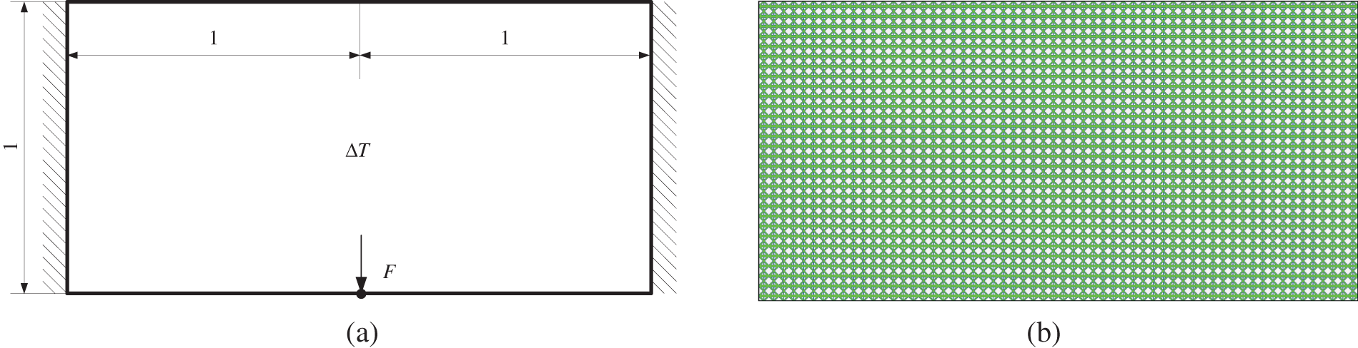
Figure 5: The first example: (a) the design problem, (b) the initial design

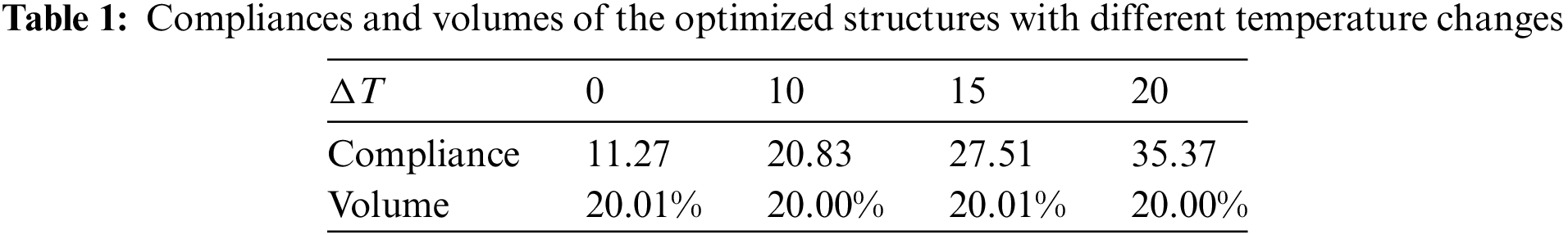
The optimized structures with different temperature changes ΔT are shown in Fig. 6, and Table 1 shows their volume and compliance values. From the results, it is clear that the optimized structures change significantly with different temperature changes, which indicates that temperature cannot be ignored in structural design. Different types of microstructures, including porous cells, empty cells, and full-solid cells, are distributed in different regions of the structure.

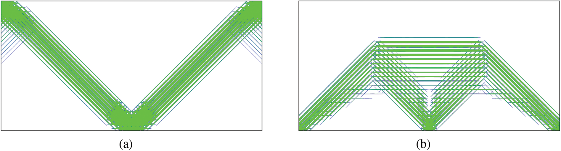
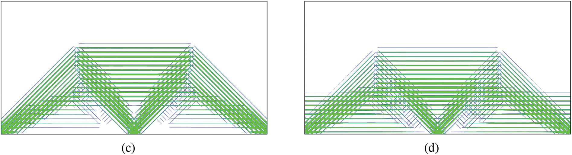
Figure 6: The optimized structure of the first example at different temperature changes: (a) ΔT = 0, (b) ΔT = 10, (c) ΔT = 15, (d) ΔT = 20

The design optimization problem is also solved only in the macroscale by using the SIMP method and the level set method. In the optimization, the temperature increment ΔT is set to 10 and the mesh used for FEA is 60×30. The optimized structures are shown in Fig. 7. The macroscale optimization results are compared with the previous one as shown in Table 2.

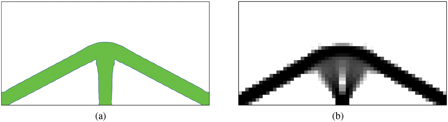
Figure 7: The optimized structures obtained through macroscale optimization methods with ΔT=10: (a) employing the level set method, (b) employing the SIMP method

As can be seen from Table 2, the level set method results in the worst structural compliance. This is because the level set-based optimization has no microstructure, which is significant for thermoelastic structure optimization. In addition, one can see in Table 2 that the allowed volume of material is not fully used with the level set method. But the material volume fraction is always kept at 20% when using the optimization method proposed in this paper. This is because the proposed method provides multiple microstructures, and the use of microstructures provides a larger degree of freedom for structural design. This allows for a more rational material distribution, which will reduce the thermal loads, increase the structural stiffness, and reduce compliance.

In the SIMP method, the relative densities of the cells are the design variables, and a penalty parameter p=3 is usually employed to drive the densities to either 1 or 0, i.e., a “black-white” design. However, as shown in Fig. 7b, the optimized structure has a large area of “gray” densities, but not a “black-white” design. Such a design is indeed the best solution given by the SIMP method, as discussed in our previous study [1]. Recall the name SIMP is “solid isotropic microstructure with penalization”, one can see that these “gray” densities represent isotropic material microstructures. Therefore, we conclude that microstructures are helpful in this optimization problem. However, the isotropic microstructures are still not enough for the optimization to fully exploit its potential, and using various anisotropic microstructures in the optimization gives the best compliance among the three methods, as shown in Table 2.

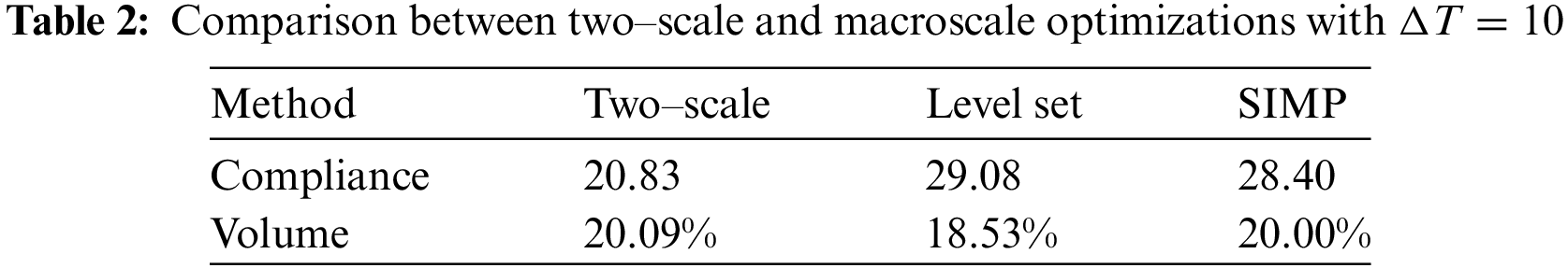
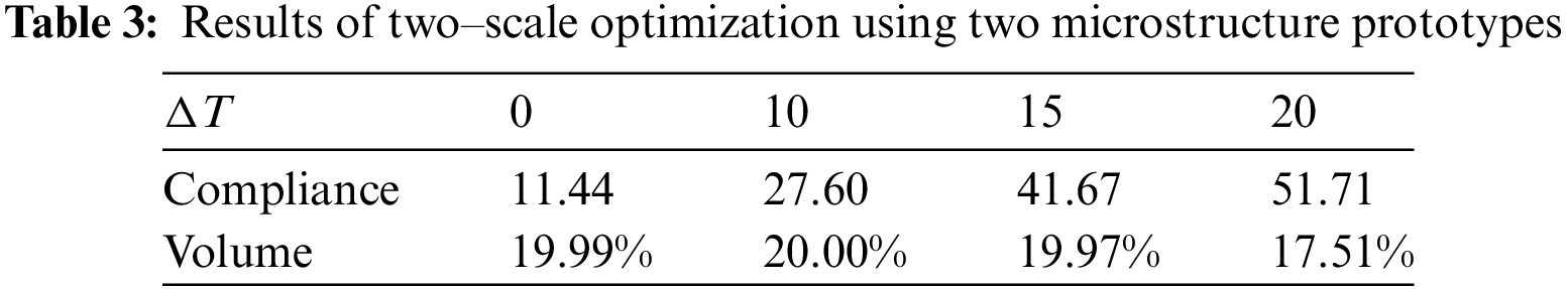
Finally, to verify the advantage of using multiple microstructure prototypes, the optimization is also conducted by using only two microstructure prototypes, as shown in Fig. 8. The setting of optimization is kept the same as before. Fig. 9 shows the optimized structures, which have the compliance and volume shown in the Table 3. Comparing Table 3 with Table 1, one can see that using more microstructural prototypes yields better optimization results. In addition, the microstructures shown in Fig. 8 are orthotropic, and those shown in Fig. 2 are anisotropic. Because anisotropic microstructures offer more flexibility than orthotropic ones, the results of the optimization with the former are better than the latter.

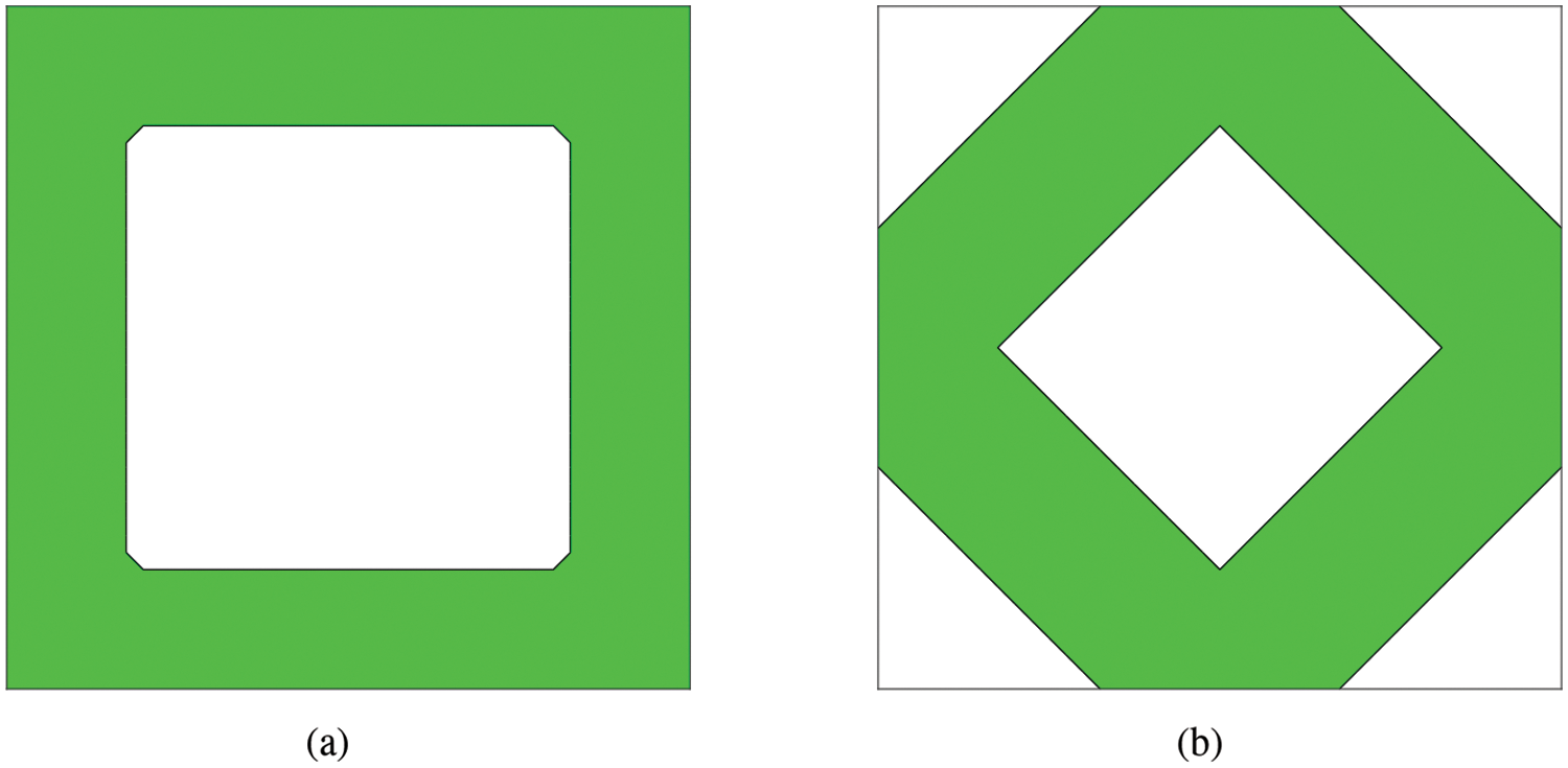
Figure 8: Two orthotropic microstructure prototypes

Figure 9: The optimized structures using two microstructure prototypes at different temperature changes: (a) ΔT = 0, (b) ΔT = 10, (c) ΔT = 15, (d) ΔT = 20

6.2 Example 2

This problem is the cantilever beam, as shown in Fig. 10. The structure is subjected to a uniform temperature change ΔT. The design domain is divided into 60×40 cells, and microstructures are defined by using the four prototypes shown in Fig. 2. In the macro-scale FEA, each cell is treated as a finite element. The upper bound of the structure volume is 50% of the design domain. The cutting heights h of all cells in the initial design are [−0.5, −0.9, −0.6, −0.6]T. The bounds of the design variables are kept the same, i.e., hmax=1.2 and hmin=−1.2. The “move” parameter is set to 0.005 when using the MMA method. The parameter δc in the convergence condition Eq. (34) is set to 0.05%.

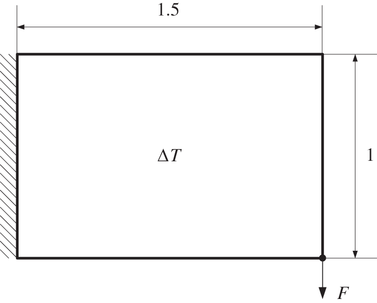
Figure 10: The design problem of the second example

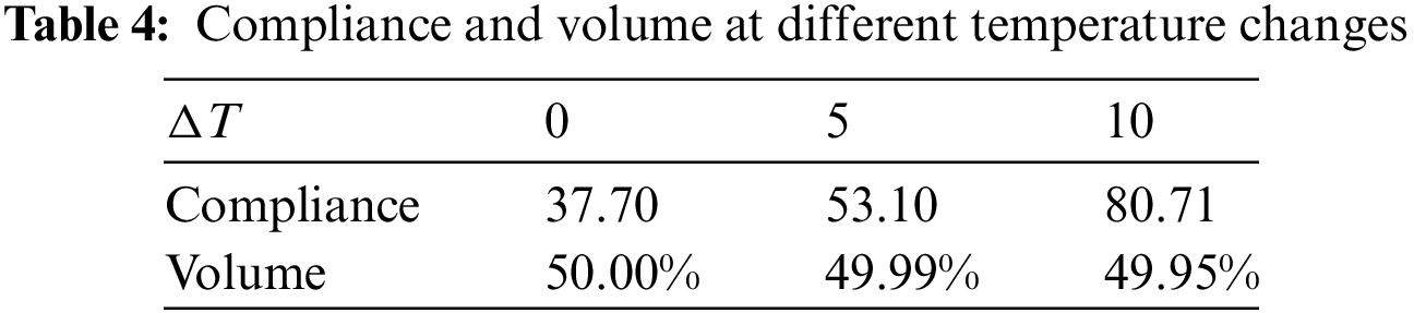
The two-scale structure is optimized with different temperature increments ΔT. The optimized results can be seen in Fig. 11, and the volume and compliance values are shown in Table 4. It is clear that as the temperature increases, the number of full-solid cells gradually decreases and that of the porous cells increases. Therefore, one can see the significance of two-scale optimization for thermoelastic structures, which considers the microstructure in the optimization.

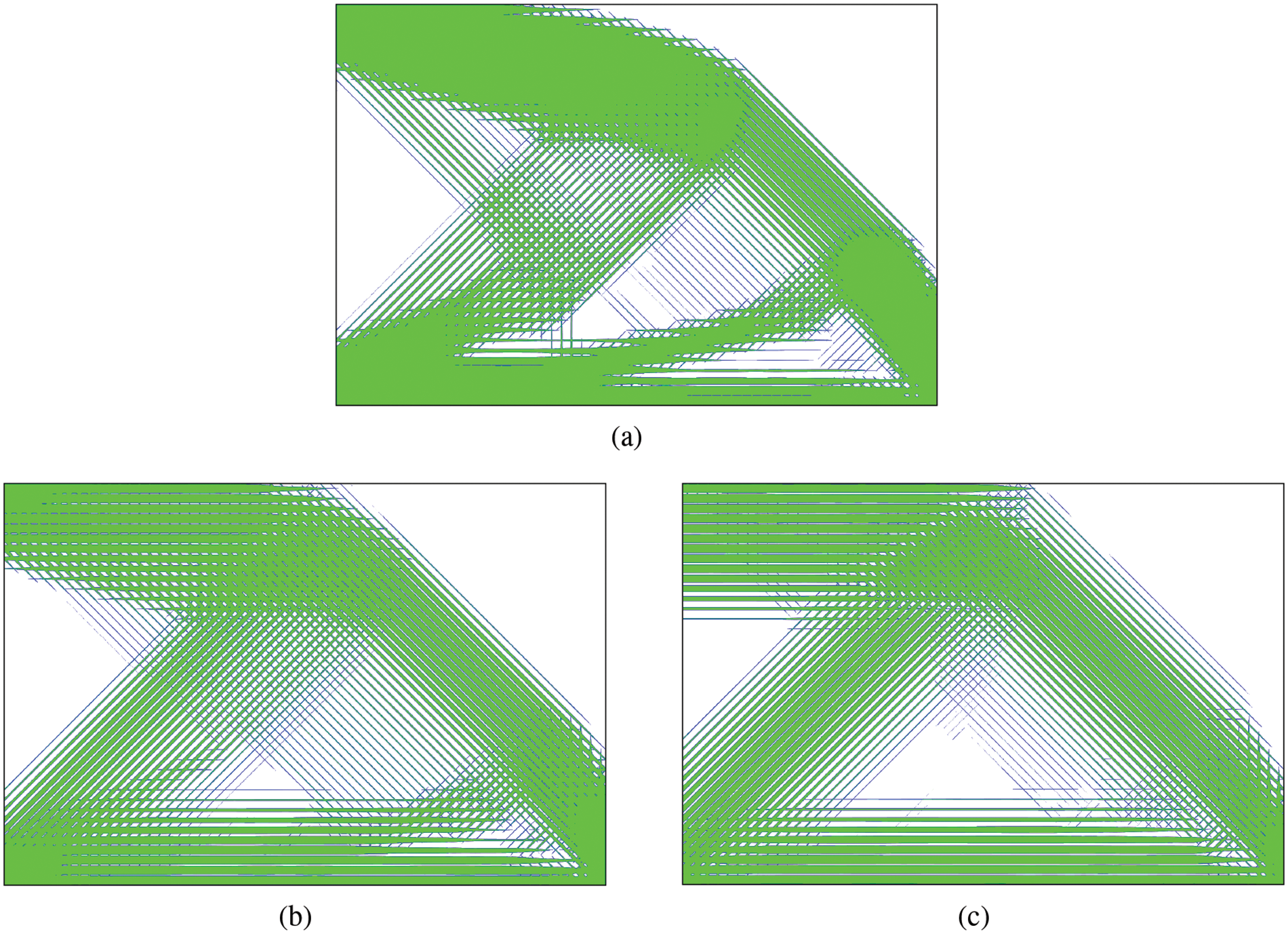
Figure 11: The optimized structure of the second example at different temperature changes: (a) ΔT = 0, (b) ΔT = 5, (c) ΔT = 10

6.3 Example 3

The previous numerical examples are all planar problems, but the approach presented in this paper can also be applied to three-dimensional (3D) problems, shown in Fig. 12. The boundary conditions for this problem are similar to those of Example 1: the two end faces of the structure are completely fixed, the middle of the bottom is subjected to a line load, and the structure is in a uniform temperature increment ΔT. The design domain is divided into 30×15×5 cells, which are also used as finite elements in FEA. The upper bound of the structure volume is set to 20% of the design domain. Young’s modulus of the material is set to E=200(Pa) and the coefficient of thermal expansion α=15.4×10−5(/K).

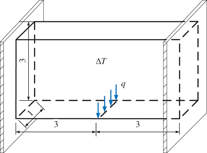
Figure 12: The 3D design problem of the third example

When the temperature increments ΔT are set to 5 and 10, the optimized structure is shown in Fig. 13. The microstructures of different regions in the structure are different, which is the result of the two-scale optimization. It is evident that in the upper face of Fig. 13a, the material in the middle of the structure was removed. As the temperature increases, more porous microstructures appear in Fig. 13b, which is the same tendency as in Fig. 9. The material distribution of the structure can also be clearly shown from the frontal views Fig. 13c,d, which are similar to the results of the planar examples. At the same time, the data-driven approach enhances the speed of structure optimization.

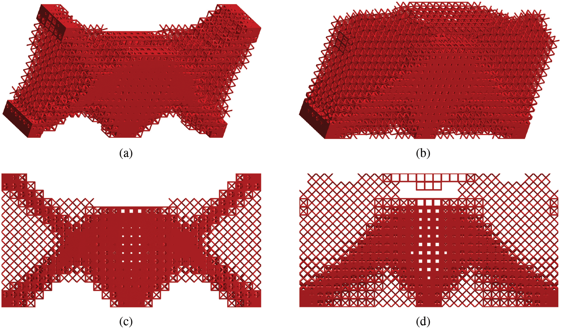
Figure 13: The optimized 3D structure at different temperature changes: (a) optimized result for ΔT=5 in the default view, (c) is the front view; (b) optimized result for ΔT=10 in the default view, (d) is the front view

7  Conclusion

In this paper, a data-driven model is integrated with the M–VCUT level set-based geometry model to solve the two–scale topology optimization of thermoelastic structures. The geometry of the microstructures is described using the M–VCUT level set method; the effective properties of the microstructure are calculated using the homogenization method in an offline phase; the RBF-based interpolation is employed to construct a data-driven model that describes the relationship between design variables and effective properties; this data-driven model is used in the FEA and sensitivity analysis. Because the costs of invoking such a data-driven model are much less than those of homogenization, the computational efficiency is improved.

From the numerical examples, one can see that the results of the proposed method are better than those of the macroscale optimization because various anisotropic microstructures are reasonably distributed into the macrostructure. In addition, one can also see that when more microstructure prototypes are used in the optimization, the results become better. Although four microstructure prototypes are used in the numerical examples in this study, the number and type of microstructure prototypes are unrestricted, and this flexibility is very important for obtaining better results in two-scale optimization.

Acknowledgement: The authors express their gratitude to Krister Svanberg for providing the MMA code support that allowed us to use it in this study.

Funding Statement: This research work is supported by the National Natural Science Foundation of China (Grant No. 12272144).

Author Contributions: The authors confirm contribution to the paper as follows: study conception and design: Jin Zhou, Qi Xia; data collection: Minjie Shao; analysis and interpretation of results: Jin Zhou, Minjie Shao, Ye Tian; draft manuscript preparation: Jin Zhou, Qi Xia. All authors reviewed the results and approved the final version of the manuscript.

Availability of Data and Materials: All data generated or analyzed during this study are included in this published article.

Ethics Approval: Not applicable.

Conflicts of Interest: The authors declare that they have no conflicts of interest to report regarding the present study.

References

1. Xia Q, Wang MY. Topology optimization of thermoelastic structures using level set method. Comput Mech. 2008;42:837–57. [Google Scholar]

2. Meng L, Zhang W, Quan D, Shi G, Tang L, Hou Y, et al. From topology optimization design to additive manufacturing: today’s success and tomorrow’s roadmap. Arch Comput Methods Eng. 2020;27:805–30. [Google Scholar]

3. Wu J, Sigmund O, Groen JP. Topology optimization of multi-scale structures: a review. Struct Multidiscipl Optim. 2021;63:1455–80. [Google Scholar]

4. Bendse MP, Kikuchi N. Generating optimal topologies in structural design using a homogenization method. Comput Methods Appl Mech Eng. 1988;71:197–224. [Google Scholar]

5. Chellappa S, Diaz AR, Bendse MP. Layout optimization of structures with finite-sized features using multiresolution analysis. Struct Multidiscip Optim. 2004;26:77–91. [Google Scholar]

6. Zhang P, Toman J, Yu Y, Biyikli E, Kirca M, Chmielus M, et al. Efficient design-optimization of variable-density hexagonal cellular structure by additive manufacturing: theory and validation. ASME J Mech Des. 2015;137:21004. [Google Scholar]

7. Wang YJ, Arabnejad S, Tanzer M, Pasini D. Hip implant optimization design with three-dimensional porous material of graded density. AMSE J Mech Des. 2018;140:111406. [Google Scholar]

8. Olhoff N, Ronholt E, Scheel J. Topology optimization of three-dimensional structures optimum microstructures. Struct Optim. 1998;16:1–18. [Google Scholar]

9. Rozvany GIN. Aims, scope, methods, history and unified terminology of computer-aided topology optimization in structural mechanics. Struct Multidiscip Optim. 2001;21:90–108. [Google Scholar]

10. Wang YJ, Xu H, Pasini D. Multiscale isogeometric topology optimization for lattice materials. Comput Methods Appl Mech Eng. 2017;316:568–85. [Google Scholar]

11. Wu ZJ, Xia L, Wang ST, Shi TL. Topology optimization of hierarchical lattice structures with substructuring. Comput Methods Appl Mech Eng. 2019;345:602–17. doi:10.1016/j.cma.2018.11.003. [Google Scholar] [CrossRef]

12. Li D, Liao W, Dai N, Xie YM. Anisotropic design and optimization of conformal gradient lattice structures. Comput-Aided Des. 2020;119:102787. doi:10.1016/j.cad.2019.102787. [Google Scholar] [CrossRef]

13. Wang J, Zhu J, Meng L, Sun QX, Liu T, Zhang WH. Topology optimization of gradient lattice structure filling with damping material under harmonic frequency band excitation. Eng Struct. 2024;309:118014. doi:10.1016/j.engstruct.2024.118014. [Google Scholar] [CrossRef]

14. Pantz O, Trabelsi K. A post-treatment of the homogenization method for shape optimization. SIAM J Control Optim. 2008;47(3):1380–98. doi:10.1137/070688900. [Google Scholar] [CrossRef]

15. Groen JP, Sigmund O. Homogenization-based topology optimization for high-resolution manufacturable microstructures. Int J Numer Methods Eng. 2018;113(8):1148–63. doi:10.1002/nme.5575. [Google Scholar] [CrossRef]

16. Allaire G, Geoffroy-Donders P, Pantz O. Topology optimization of modulated and oriented periodic microstructures by the homogenization method. Comput Math Appl. 2019;78:2197–229. doi:10.1016/j.camwa.2018.08.007. [Google Scholar] [CrossRef]

17. Zhu Y, Li S, Du Z, Liu C, Guo X, Zhang W. A novel asymptotic-analysis-based homogenisation approach towards fast design of infill graded microstructures. J Mech Phys Solids. 2019;124:612–33. doi:10.1016/j.jmps.2018.11.008. [Google Scholar] [CrossRef]

18. Geoffroy-Donders P, Allaire G, Pantz O. 3-D topology optimization of modulated and oriented periodic microstructures by the homogenization method. J Comput Phys. 2020;401:108994. doi:10.1016/j.jcp.2019.108994. [Google Scholar] [CrossRef]

19. Rodrigues HC, Guedes JM, Bendse MP. Hierarchical optimization of material and structure. Struct Multidiscip Optim. 2002;24:1–10. doi:10.1007/s00158-002-0209-z. [Google Scholar] [CrossRef]

20. Coelho PG, Fernandes PR, Guedes JM, Rodrigues HC. A hierarchical model for concurrent material and topology optimisation of three-dimensional structures. Struct Multidiscip Optim. 2008;35:107–15. doi:10.1007/s00158-007-0141-3. [Google Scholar] [CrossRef]

21. Xia L, Breitkopf P. Concurrent topology optimization design of material and structure within FE2 nonlinear multiscale analysis framework. Comput Methods Appl Mech Eng. 2014;278:524–42. [Google Scholar]

22. Li H, Luo Z, Zhang N, Gao L, Brown T. Integrated design of cellular composites using a level-set topology optimization method. Comput Methods Appl Mech Eng. 2016;309:453–75. [Google Scholar]

23. Wang YG, Kang Z. Concurrent two-scale topological design of multiple unit cells and structure using combined velocity field level set and density model. Comput Methods Appl Mech Eng. 2019;347:340–64. [Google Scholar]

24. Zhou SW, Li Q. Design of graded two-phase microstructures for tailored elasticity gradients. J Mater Sci. 2008;43:5157–67. [Google Scholar]

25. Zhou SW, Li Q. Microstructural design of connective base cells for functionally graded materials. Mater Lett. 2008;62:4022–4. [Google Scholar]

26. Radman A, Huang X, Xie YM. Topology optimization of functionally graded cellular materials. J Mater Sci. 2013;48:1503–10. doi:10.1007/s10853-012-6905-1. [Google Scholar] [CrossRef]

27. Cramer AD, Challis VJ, Roberts AP. Microstructure interpolation for macroscopic design. Struct Multidiscip Optim. 2016;53:489–500. doi:10.1007/s00158-015-1344-7. [Google Scholar] [CrossRef]

28. Wang YQ, Chen FF, Wang MY. Concurrent design with connectable graded microstructures. Comput Methods Appl Mech Eng. 2017;317:84–101. doi:10.1016/j.cma.2016.12.007. [Google Scholar] [CrossRef]

29. Liu H, Zong H, Shi T, Xia Q. M-VCUT level set method for optimizing cellular structures. Comput Methods Appl Mech Eng. 2020;367:113154. doi:10.1016/j.cma.2020.113154. [Google Scholar] [CrossRef]

30. Xia Q, Zong H, Shi T, Liu H. Optimizing cellular structures through the M-VCUT level set method with microstructure mapping and high order cutting. Compos Struct. 2021;261:113298. doi:10.1016/j.compstruct.2020.113298. [Google Scholar] [CrossRef]

31. Andreassen E, Andreasen CS. How to determine composite material properties using numerical homogenization. Comput Mater Sci. 2014;83:488–95. doi:10.1016/j.commatsci.2013.09.006. [Google Scholar] [CrossRef]

32. Wendland H. Piecewise polynomial, positive definite and compactly supported radial functions of minimal degree. Adv Comput Math. 1995;4:389–96. doi:10.1007/BF02123482. [Google Scholar] [CrossRef]

33. Buhmann MD. Radial basis functions: theory and implementations. In: Cambridge monographs on applied and computational mathematics. New York, NY: Cambridge University Press; 2004. vol. 12. [Google Scholar]

34. Wang SY, Wang MY. Radial basis functions and level set method for structural topology optimization. Int J Numer Meth Eng. 2006;65:2060–90. doi:10.1002/nme.1536. [Google Scholar] [CrossRef]

35. Luo Z, Tong LMY, Wang SYW. Shape and topology optimization of compliant mechanisms using a parameterization level set method. J Comput Phys. 2007;227:680–705. doi:10.1016/j.jcp.2007.08.011. [Google Scholar] [CrossRef]

36. Wei P, Li Z, Li X, Wang MY. An 88-line MATLAB code for the parameterized level set method based topology optimization using radial basis functions. Struct Multidiscip Optim. 2018;58:831–49. doi:10.1007/s00158-018-1904-8. [Google Scholar] [CrossRef]

37. Jiu L, Zhang W, Meng L, Zhou Y, Chen L. A CAD-oriented structural topology optimization method. Comput Struct. 2020;239:106324. doi:10.1016/j.compstruc.2020.106324. [Google Scholar] [CrossRef]

38. Tian Y, Shi T, Xia Q. Buckling optimization of curvilinear fiber-reinforced composite structures using a parametric level set method. Front Mech Eng. 2024;19(1):1–12. doi:10.1007/s11465-023-0780-0. [Google Scholar] [CrossRef]

39. Yan J, Guo X, Cheng G. Multi-scale concurrent material and structural design under mechanical and thermal loads. Comput Mech. 2016;57:437–46. doi:10.1007/s00466-015-1255-x. [Google Scholar] [CrossRef]

40. Xu B, Huang X, Zhou S, Xie YM. Concurrent topological design of composite thermoelastic macrostructure and microstructure with multi-phase material for maximum stiffness. Compos Struct. 2016;150:84–102. doi:10.1016/j.compstruct.2016.04.038. [Google Scholar] [CrossRef]

41. Jiang H, Wei B, Zhou E, Wu Y, Li X. Robust topology optimization for thermoelastic hierarchical structures with hybrid uncertainty. J Thermal Stresses. 2021;44(12):1458–78. doi:10.1080/01495739.2021.1999877. [Google Scholar] [CrossRef]

42. Deng J, Yan J, Cheng G. Multi-objective concurrent topology optimization of thermoelastic structures composed of homogeneous porous material. Struct Multidiscip Optim. 2013;47:583–97. doi:10.1007/s00158-012-0849-6. [Google Scholar] [CrossRef]

43. Yan J, Sui Q, Fan Z, Duan Z. Multi-material and multiscale topology design optimization of thermoelastic lattice structures. Comp Model Eng Sci. 2022;130(2):967–86. doi:10.32604/cmes.2022.017708. [Google Scholar] [CrossRef]

44. Zheng J, Ding S, Jiang C, Wang Z. Concurrent topology optimization for thermoelastic structures with random and interval hybrid uncertainties. Int J Numer Methods Eng. 2022;123(4):1078–97. doi:10.1002/nme.6889. [Google Scholar] [CrossRef]

45. Sigmund O. Design of material structures using topology optimization (PhD Thesis). Technical University of Denmark: Denmark; 1994. [Google Scholar]

46. Svanberg K. The method of moving asymptotes-a new method for structural optimization. Int J Numer Methods Eng. 1987;24(2):359–73. doi:10.1002/nme.1620240207. [Google Scholar] [CrossRef]

47. Liu H, Chen L, Bian H. Data-driven M-VCUT topology optimization method for heat conduction problem of cellular structure with multiple microstructure prototypes. Int J Heat Mass Transf. 2022;198:123421. doi:10.1016/j.ijheatmasstransfer.2022.123421. [Google Scholar] [CrossRef]