An Efficient Technique for One-Dimensional Fractional Diffusion Equation Model for Cancer Tumor

1  Introduction

The generalization of integer order calculus to any arbitrarily large order referred to as fractional calculus (FC). It is an exciting subject in mathematics because of its capacity to precisely describe a wide range of non-linear phenomena. Fractional derivatives appeared in 1695; it has been found that FC is superior to classical calculus for modeling real-world problems and presents a systematic and effective exposition of nature’s reality. The application of FC is detected in numerous branches of science and engineering. FC has currently gained more attention in electrodynamics [1], signal processing [2], fluid dynamics [3], chaos behavior [4], financial models [5], optics [6], a noisy environment [7], economics [8], neurophysics [9], and many others [10–14]. FC describes new features of a complex biological model and plays a significant role in obtaining the memory and hereditary features of the system. Fractional differential equations (FDEs) with space, time, or any other variable dependent order have been successfully employed to examine time or space-dependent dynamics. FDE models have been widely recognized as a novel and precise way of accurately representing real-world occurrences. The fractional model of the diffusion problem is crucial in studying the cancer model.

Cancer is one of the most lethal diseases in the world today, with no cure and a complex structure that limits cancer-fighting success. Cancer is a broad category of diseases characterized by uncontrolled cell proliferation that also produces dangerous tumors. Many cancers include antigens that can be identified by the adaptive immune system and, hence, exploited to stimulate an anticancer immune response. However, the interactions between tumor cells and other tumors are extremely complicated and dynamic. So, cancer treatment or cure has proven to be an exhausting task. Arshad et al. [15] applied a multi-step generalized differential transform method (MSGDTM) to the non-linear model of the growth of tumor cells and focused on enhancing immunogenic behavior through exogenous input. Rihan et al. [16] found delay differential equations (DDEs) to elaborate on the interconnection between the effectors and the tumor cells. The least square method solves the problem of parameter estimation for a given actual observation.

Diseases such as malaria, dengue fever, HIV infection, influenza, Ebola virus, cancer, and others were dealt with ordinary differential equations of integer order, but a short time ago, more concentration were defined in fractional order. The mathematical models that use fractional differential equations are crucial for explaining how tumors spread and connect with one another. The fractional tumor model interprets the tumor and effector cells and gives a relative and chaotic study of cells, which explains the killing rate of cancer cells [17–20]. Farman et al. [21] focused their research on a model of fractional-order immunotherapy bladder with a vaccination strategy for cancer in the sense of Caputo fractional derivative. The result indicates that the fractional order significantly changes disease control in the early stages. Panchal et al. [22] applied the differential transform method (DTM) to the fractional cancer model, explained the outcomes of chemotherapy, and revealed that if the chemotherapy drug concentration is inappropriate, then the growth of tumor cells increases in a large number or may cause a decrease in effector cells. Ndenda et al. [23] used the Adams-Bashforth-Moulton method of fractional order for the tumor immune interaction to treat the cytokine interleukin 2 (1L-2). The high concentration of 1L-2 may nurture the body’s immune system, but it has certain side effects. Results state that satisfactory tumor control can be achieved through this method. Korpinar et al. [24] used the residual power series method (RPSM) to obtain the series solution of the cancer model via fractional-order. The RPSM is described with Maclaurin’s expansion and covers complex computational work. Ali Dokuyucu et al. [25] examined the cancer treatment model and converted the model into fractional order, where the differential operator is defined in Caputo-Fabrizio to obtain the solution. They reported that fractional derivatives provide beneficial details about the process. Saadeh et al. [26] presented the analytical series solution of the cancer model by considering the Laplace RPSM. They investigated the fractional-order derivatives of the time-dependent cancer cell concentrations and concluded that the percentage of apparent cell death can also be affected by the concentration of cancer cells. Abaid Ur Rehman et al. [27] used the method called reduced differential transform method for the tumor model in the frame of the FC, which explains the connection between chemotherapeutic agents, normal cells, tumor cells, and immune cells and obtained a solution in the sense of Caputo. Padder et al. [28] analyzed the tumor growth and assessed the prospective treatment of the fractional tumor model using the Caputo-derivative. The obtained outcome depicts disease transmission dynamics as manifested in the relationships among macrophages and tumors.

This research considers a diffusion-based model proposed by [29] within the confines of a spherical tumor with the rate of intensification specified by p and the percentage of death resulting from therapy indicated by k and presumed in the below equation:

∂u(ζ,t)∂t=pu(ζ,t)−ku(ζ,t)+D1r2∂∂r(r2∂u(ζ,t)∂r),(1)

where the diffusion coefficient is symbolized by D, concentration of cancerous cells at r point, and the time t is given by u(ζ,t). In most studies, therapy is only permitted as a time function. Moyo et al. [30] changed this to make it function for both the time and position of the cancerous cells, which is a more reasonable assumption and look at the previously mentioned equation as a one-dimensional model with variable killing percentage using the Lie point symmetry method. This study considers the fractional modification of the cancer tumor model with diffusion equation

Dtαcu(ζ,t)=∂2u(ζ,t)∂ζ2−k(ζ,t)u(ζ,t),(2)

where Dtαc is the Caputo fractional derivative, k(ζ,t) is described as the remedy’s temporal profile and k(ζ,t)u(ζ,t) denotes the rate at which tumor cells are removed. Two cases of the cancer cells killing ratio k(ζ,t) were discussed. k is merely a time function and k is proportional to cell concentration.

Odibat [31] considered linear and non-linear fractional models with the aid of the homotopy analysis method (HAM) and the variational iteration method. They produced the results in the Caputo sense, contributing to the non-linear FDEs that can be solved using these techniques. Iyiola et al. [32] considered the cancer tumor model and implemented the HAM. They found that fractional order derivatives are more helpful than classical order derivatives. Arqub et al. [33] analyzed a susceptible-infected-recovered (SIR) fractional order epidemic model. The homotopy analysis method was considered to study the analytical series solution by including an auxiliary parameter. Abdl-Rahim et al. [34] adopted the combination of two methods, HAM and natural transform method (NTM), by considering auxiliary parameters, which gives the solution of epidemiology models. Based on the above HAM outcomes, the secured result displays the requirement of an additional parameter that offers more flexibility in adjusting homotopy expansion, leading to faster convergence and improved solution reliability. Hence, this study has applied q-homotopy analysis transform method (q-HATM), which is more effective in solving FDEs. q-HATM executes a crucial role in the fractional order epidemic model, and they reported that fractional calculus is an authoritative and precise strategy to examine the conduct of diseases affecting people compared with classical calculus. This study confirms the pertinence and consequence of fractional operators for real-world problems. It indicates that the proposed method benefits numerous scientific fields [35–38]. Veeresha et al. [39] employed the q-HATM for fractional coupled systems arising in magneto-thermoelasticity, which gives the fast convergent series solution and the efficacy of the preferred novel approach. The outcomes are described graphically to understand the behavior of the system. Compared to other techniques, this gives a feasible and significant outcome and is highly efficient. Seddek et al. [40] and Yasmin et al. [41] analyzed that q-HATM is a dynamic tool to resolve the models of fractional order and prevail over difficulties in acquiring solutions because of non-locality and non-linearity, so the method is ideal.

The primary objective of the current research is to find an analytical solution for the considered time fractional-order cancer model using q-HATM. This particular model has yet to be explored by q-HATM. There are various techniques to solve fractional models, but they have limitations, perturbations, huge time of simplification, discretization, assumptions, and many others. However, the considered technique is free from the above limitations. Many researchers have shown that the proposed method is effectively and widely employed in various models. It also shows that the proposed technique reduces complexity and computational work, making it a more reliable and efficient tool for simulating the fractional order differential model. It combines the positive aspects of both analytical as well as numerical approaches. It offers an analytical solution defined in terms of a convergence series and allows for numerical approximation when necessary.

The current paper is assembled as follows: Section 1 includes an introduction. Basic definitions and preliminaries are given in Section 2. Section 3 outlines the methodology of the preferred method. Section 4 discusses the uniqueness and convergence of the considered model. Section 5 describes some examples to show the efficiency of the projected technique and their results with graphs. The discussion part of the obtained graphical and numerical results with their significance is added in Section 6. Section 7 is the conclusion.

2  Preliminaries

This section presents the basic definitions of the fractional-order operator and the Laplace transform.

Definition 2.1. For a function g(t)∈C−1n, the fractional integral of order α≥0 in terms of Podlubny [42] is specified as follows:

Iαg(t)=1Γ(α)∫0t(t−τ)α−1g(n)(τ)dτ,t>0,α>0,(3)

I0g(t)=g(t),

where Γ(•) indicates the Gamma function.

Definition 2.2. In terms of Caputo, the function g∈C−1n with fractional derivative is outlined below [42]:

Dtαg(t)={dng(t)dtn,α=n∈N,1Γ(n−α)∫0t(t−τ)n−α−1g(n)(τ)dτ,n−1<α<n,n∈N.(4)

The linear property of the Caputo fractional derivative is as follows:

Dcα(λx(t)+μy(t))=λDcαx(t)+μDcαy(t),

where λ and μ are some constants.

Definition 2.3. A Caputo fractional derivative’s Laplace transform (LT) [43,44] for the function Dtαg(t) is stated as follows:

L[Dtαg(t)]=sαG(s)−∑γ=0n−1sα−γ−1g(γ)(0+),(n−1<α≤n),(5)

where G(s) is the function g(t)’s LT.

3  Fundamental Procedure for the Suggested Method

This part of the paper illustrates the solution algorithm of the q-HATM technique. It considers a general non-linear and non-homogeneous differential equation in the frame of fractional-order, which is in the form given below:

DtαCν(ζ,t)+Rν(ζ,t)+Nν(ζ,t)=g(ζ,t),0<α≤1,(6)

where DtαCv(ζ,t) signifies the fractional derivative in terms of Caputo of the function v(ζ,t), g(ζ,t) is indicated as source terms, the non-linear differential operator is denoted by N, and R is the linear differential operator which is bounded in ζ and t.

By implementing the LT on Eq. (6), the following can be obtained:

sαL[ν(ζ,t)]−∑k=0n−1sα−k−1ν(k)(ζ,t)+L[Rν(ζ,t)+Nν(ζ,t)]=L[g(ζ,t)].(7)

On simplifying Eq. (7), then

L[ν(ζ,t)]−1sα∑k=0n−1sα−k−1νk(ζ,0)+1sα{L[Rν(ζ,t)+Nν(ζ,t)−g(ζ,t)]}=0.(8)

In relation to the HAM, the non-linear operator N is presented in the following manner:

N[ϕ(ζ,t;q)]=L[ϕ(ζ,t;q)]−1sα∑k=0n−1sα−k−1ϕk(ζ,t;q)(0+)+1sα{L[Rϕ(ζ,t;q)+Nϕ(ζ,t;q)]−g(ζ,t)]},(9)

where ϕ(ζ,t;q) specifies the real function for ζ, t and q, q∈[0,1n](n≥1).

The equation for deformation of zero’th-order having H(ζ,t) is characterized as follows:

L[ϕ(ζ,t;q)−ν0(ζ,t)](1−nq)=ℏqN[ϕ(ζ,t;q)]H(ζ,t),(10)

where initial guess of ν(ζ,t) is ν0(ζ,t), ϕ(ζ,t;q) is an unidentified function, q∈[0,1n] is the embedding parameter, L is the LT and ℏ≠0 (auxiliary parameter). Regarding q=0 and q=1n, the subsequent outcomes are achieved:

ϕ(ζ,t;0)=v0(ζ,t), ϕ(ζ,t;1n)=v(ζ,t).(11)

Hence, from the solution v0(ζ,t) to v(ζ,t), the solution ϕ(ζ,t;q) converges by varying q between 0 and 1n. Then, the function ϕ(ζ,t;q) in series form is extended as follows by employing Taylor’s theorem throughout q

ϕ(ζ,t;q)=v0(ζ,t)+∑m=1∞qmvm(ζ,t),(12)

where

vm(ζ,t)=1m!(∂mϕ(ζ,t;q)∂qm|q=0).(13)

By a specific choice of auxiliary parameter ℏ and n, auxiliary linear operator, the initial estimation v0(ζ,t) and H(ζ,t) appropriately, the series (12) converges at q=1n provides the solution to the original non-linear Eq. (6) of the type

v(ζ,t)=v0(ζ,t)+∑m=1∞vm(ζ,t)(1n)m.(14)

The next step is to differentiate the deformation Eq. (10) up to m-times with regard to q, afterwards divide by m! and ultimately taking q=0, this study acquires the equation which is in deformation form of order m as follows:

L[vm(ζ,t)−kmvm−1(ζ,t)]=ℏH(ζ,t)ℜm(v→m−1),(15)

where

ℜm(v→m−1)=1(m−1)!∂m−1N[ϕ(ζ,t;q)]∂qm−1|q=0,(16)

and

km={0,m≤1,n,m>1.(17)

Vectors are regarded in the following way:

ν→m={ν0(ζ,t),ν1(ζ,t),…,νm(ζ,t)}.(18)

By employing an inverse LT to the deformation Eq. (15), which yields the recursive equation and can be expressed as follows:

νm(ζ,t)=kmνm−1(ζ,t)+ℏL−1[H(ζ,t)ℜm(ν→m−1)].(19)

Finally, by resolving Eq. (19), the νm(ζ,t) iterative terms can be attained. This is how the q-HATM series solution is described:

ν(ζ,t)=∑m=0∞νm(ζ,t).(20)

4  Uniqueness and Convergence of Solution for Cancer Tumor Model

Theorem 4.1: Uniqueness theorem

For the fractional-order differential Eq. (2) under consideration, the solution obtained by q-HATM is unique, for every λ∈(0,1), where λ=(km+ℏ)+ℏ(δ2+k)T.

Proof: The solution to Eq. (2) is given by

g(ζ,t)=∑m=0∞gm(ζ,t),

where

gm(ζ,t)=(km+ℏ)gm−1(ζ,t)−(1−kmn)L−1(∑k=0n−1sα−k−1(g(k)(ζ,0)))+ℏL−1[1sαL{∂2gm−1(ζ,t)∂ζ2−kgm−1(ζ,t)}].(21)

Now, suppose g and g∗ are different solutions of Eq. (2), then demonstrating that g=g∗ suffices to validate the theorem. Then, using Eq. (21), it can have

|g−g∗|=|(km+ℏ)(g−g∗)+ℏL−1[1sαL{(∂2g∂ζ2−∂2g∗∂ζ2)−k(g−g∗)}]|.

Then, implementing the convolution theorem for LT, it can obtain

|g−g∗|=(km+ℏ)|g−g∗|+ℏ∫0t(|(∂2g∂ζ2−∂2g∗∂ζ2)−k(g−g∗)|)(t−ξ)αΓ(α+1)dξ

|g−g∗|≤(km+ℏ)|g−g∗|+ℏ∫0t(|∂2g∂ζ2−∂2g∗∂ζ2|+|−k(g−g∗)|)(t−ξ)αΓ(α+1)dξ≤(km+ℏ)|g−g∗|+ℏ∫0t(δ2|(g−g∗)|+k|(g−g∗)|)(t−ξ)αΓ(α+1)dξ.

where δ2=∂2∂ζ2.

With the help of the integral mean value theorem [45,46], the preceding expression could be written in the following way:

|g−g∗|≤(km+ℏ)|g−g∗|+ℏ(δ2|(g−g∗)|+k|(g−g∗)|)T.

Here λ=(km+ℏ)+ℏ(δ2+k)T, as a result

|g−g∗|≤λ|g−g∗|

|g−g∗|(1−λ)≤0.

In view of the fact that 0<λ<1, then g−g∗=0⇒g=g∗.

As a result, Eq. (2) has a unique solution.

Theorem 4.2: Convergence theorem

Consider a Banach space denoted by E, non-linear mapping X:E→E and then presume that

‖X(g)−X(l)‖≤λ‖g−l‖,∀a,b∈E.

After that, X has a fixed point in accordance with Banach’s fixed point theory. In addition, the sequence of the q-HATM solution converges to a specific point of X with any of the choices of a0,b0∈E and then

‖gm−gn‖≤λn1−λ‖g1−g0‖,∀a,b∈E.

Proof: Let us consider (E[J],‖.‖), which contains every continuous functions on J and that its norm is symbolised as ‖z(t)‖=maxt∈J|z(t)|. At the outset, we point out that {gn} in E is a Cauchy sequence.

Now consider,

‖gm−gn‖=maxt∈J|gm−gn|=maxt∈J|(gm−1−gn−1)(km+h)+ℏL−1(1sαL((∂2gm−1∂ζ2−∂2gn−1∂ζ2)−k(gm−1−gn−1)))|≤maxt∈J[|(gm−1−gn−1)|(km+h)+ℏL−1(1sαL(|∂2gm−1∂ζ2−∂2gn−1∂ζ2|+k|(gm−1−gn−1)|))].

According to the convolution theorem for Laplace, the following can be obtained:

‖gm−gn‖≤maxt∈J[|(gm−1−gn−1)|(km+h)+ℏ∫0t(|∂2gm−1∂ζ2−∂2gn−1∂ζ2|+k|(gm−1−gn−1)|)(t−ξ)αΓ(α+1)dξ]≤maxt∈J[|(gm−1−gn−1)|(km+h)+ℏ∫0t(δ2|(gm−1−gn−1)|+k|(gm−1−gn−1)|)(t−ξ)αΓ(α+1)dξ].

Using the integral mean value theorem [45,46], the inequality above becomes

‖gm−gn‖≤maxt∈J[|(gm−1−gn−1)|(km+h)+ℏ(δ2|(gm−1−gn−1)|+k|(gm−1−gn−1)|)T]≤λ‖gm−1−gn−1‖.

For m=n+1, one could obtain

‖gn+1−gn‖≤λ‖gn−gn−1‖≤λ2‖gn−1−gn−2‖≤λ3‖gn−2−gn−3‖≤....≤λn‖g1−g0‖.

By applying triangular inequality, it yields:

‖gm−gn‖≤‖gm−gm−1‖+‖gm+1−gm‖+…+‖gn+2−gn+1‖+‖gn+1−gn‖≤[λn+λn+1+…+λm−1]‖g1−g0‖=λn[1+λ+…+λm−n−1]‖g1−g0‖≤λn[1−λm−n−11−λ]‖g1−g0‖.

As 0<λ<1, obviously 1−λm−n−1<1, then inequality becomes

‖gm−gn‖≤λn1−λ‖g1−g0‖.

But ‖g1−g0‖<∞, consequently, as m<∞ then ‖gm−gn‖→0.

As a result, the sequence {gn} in E[J] is the Cauchy sequence. Therefore, {gn} is a convergent sequence (because every Cauchy sequence is a convergent sequence), and this yields the end of the required results.

5  Solution for Fractional-Order Cancer Tumor Models

The analytical solutions of the suggested fractional cancer model are discussed in this section using Mathematica software. This study implements the q-HATM technique to observe the accuracy and effectiveness and presents graphs of the obtained outcomes.

Case 5.1: Consider the equation of the cancer cell killing ratio with fractional-order, a function of time dependence only.

Dtαcu(ζ,t)=∂2u(ζ,t)∂ζ2−t2u(ζ,t),t>0,0≤ζ≤1,0<α≤1,(22)

subjected to the initial condition

u(ζ,0)=ekζ.(23)

By implementing LT in Eq. (22) and with regard to the initial constraint given in Eq. (23), then

L[u(ζ,t)]−1su(ζ,0)−1sαL{∂2u(ζ,t)∂ζ2−t2u(ζ,t)}=0.(24)

In order to use the proposed technique, N (non-linear operator) can be stated as follows:

N[ϕ(ζ,t;q)]=L[ϕ(ζ,t;q)]−1sϕ(ζ,0;q)−1sαL{∂2ϕ(ζ,t;q)∂ζ2−t2ϕ(ζ,t;q)}.(25)

After following the algorithm’s instructions, it is possible to obtain a deformation equation for mth-order in the following syntax:

L[um(ζ,t)−kmum−1(ζ,t)]=ℏ(ℜm[u→m−1(ζ,t)]),(26)

where

ℜm[u→m−1(ζ,t)]=L[um−1(ζ,t)]−(1−kmn)1su(ζ,o)−1sαL{∂2um−1(ζ,t)∂ζ2−t2um−1(ζ,t)}.(27)

On tackling with inverse LT on Eq. (26), it acquires

um(ζ,t)=kmum−1(ζ,t)+ℏ(L−1{ℜm[u→m−1(ζ,t)]}).(28)

Thus, the solution to Eq. (28) is obtained as follows:

u0(ζ,t)=ekζ,

u1(ζ,t)=ℏekζtα(2t2Γ(α+3)−k2Γ(α+1)),

u2(ζ,t)=ℏekζ(n+ℏ)tα(2t2Γ(α+3)−k2Γ(α+1))+ℏ2ekζt2α(k2Γ(α+3)−2t2Γ(α+1))2Γ(α+1)2Γ(α+3)2

u3(ζ,t)=(n+ℏ)(ℏ2ekζt2α(k2Γ(α+3)−2t2Γ(α+1))2)Γ(α+1)2Γ(α+3)2+ℏekζ(n+ℏ)2tα(2t2Γ(α+3)−k2Γ(α+1))+ℏ2ekζt2α(k2Γ(α+3)−2t2Γ(α+1))2(Γ(α+1)(Γ(α+3)(n+ℏ)+2ℏtα+2)−k2ℏΓ(α+3)tα)Γ(α+1)3Γ(α+3)3,

⋮

In this manner, it can achieve other recurrent terms. Lastly, the necessary series solution of Eq. (22) by using q-HATM can be written as follows:

u(ζ,t)=u0(ζ,t)+∑m=1∞um(ζ,t).(29)

Case 5.2: Consider the cancer tumor equation with fractional-order, where the tumor cells net killing ratio varies with the level of cell concentration.

Dtαcu(ζ,t)=∂2u(ζ,t)∂ζ2−2ζ∂u∂ζ−u2(ζ,t),0≤ζ≤1,t>0,0<α≤1.(30)

with initial settings

u(ζ,0)=ζp.(31)

Primarily, by operating LT on Eq. (30) and utilizing the initial constraint stated in Eq. (31), then

sαL[u(ζ,t)]−sα−1u(ζ,0)−L{∂2u(ζ,t)∂ζ2−2ζ∂u∂ζ−u2(ζ,t)}=0.(32)

By simplifying the above equation, it has

L[u(ζ,t)]−1su(ζ,0)−1sαL{∂2u(ζ,t)∂ζ2−2ζ∂u∂ζ−u2(ζ,t)}=0.(33)

This study specifies the non-linear operator N with the help of Eq. (33) as follows:

N[ϕ(ζ,t;q)]=L[ϕ(ζ,t;q)]−1sϕ(ζ,0;q)−1sαL{∂2ϕ(ζ,t;q)∂ζ2−2ζ∂ϕ∂ζ−ϕ2(ζ,t;q)}.(34)

By exercising the preferred procedure, the deformation equation is prescribed as follows:

L[um(ζ,t)−kmum−1(ζ,t)]=ℏℜm[u→m−1(ζ,t)].(35)

where

ℜm[u→m−1(ζ,t)]=L[um(ζ,t)]−(1−kmn)1su(ζ,0)−1sαL{∂2um−1(ζ,t)∂ζ2−2ζ∂um−1∂ζ−∑i=0m−1uium−1−i(ζ,t)}.(36)

This is a very crucial part when solving a non-linear differential equation using the homotopy technique. In Eq. (35), the inverse Laplace transform is used, and then

um(ζ,t)=kmum−1(ζ,t)+ℏ(L−1{ℜm[u→m−1(ζ,t)]}).(37)

After resolving Eq. (37), the following solution is reached:

u0(ζ,t)=ζp,

u1(ζ,t)=(−((p−1)pζp−2)+2pζp−2+ζ2p)(ℏtα)Γ(α+1),

u2(ζ,t)=(n+ℏ)(−((p−1)pζp−2)+2pζp−2+ζ2p)(ℏtα)Γ(α+1)+(ζp−4(p4−10p3+p2(31−6ζp+2)+2ζ2p+4+6p(2ζp+2−5)))(ℏ2t2α)Γ(2α+1),

u3(ζ,t)=(n+ℏ)(ζp−4(p4−10p3+p2(31−6ζp+2)+2ζ2p+4+6p(2ζp+2−5)))(ℏ2t2α)Γ(2α+1)+1Γ(2α+1)ℏ2ζp−6t3α(ζ2Γ(α+1)(n+ℏ)(p4−10p3+p2(31−6ζp+2)+2ζ2p+4+6p(2ζp+2−5))−ℏ(p6−21p5+p4(169−27ζp+2)+p3(158ζp+2−651)+p2(−299ζp+2+32ζ2p+4+1198)−5ζ3p+6−12p(−15ζp+2+4ζ2p+4+70)))+(n+ℏ)2(−((p−1)pζp−2)+2pζp−2+ζ2p)(ℏtα)Γ(α+1),

⋮

Likewise, the leftover iterative components are able to be determined. Thereafter, the necessary series solution obtained by q-HATM for the considered case of Eq. (30) is inclined as follows:

u(ζ,t)=u0(ζ,t)+∑m=1∞um(ζ,t).(38)

6  Results and Discussion

The numerical analysis of the solution u(ζ,t) derived by the technique called q-HATM for chosen cases of the cancer model with fractional order is presented in this section. The nature of the solution for Case 5.1 and Case 5.2 are represented by 3D plots. Fig. 1 depicts the response of the obtained solution of Case 5.1 with distinct α=1, 0.9, 0.8, 0.7. It look into the effect of time fractional order on the net killing rate of cancerous cells. Fig. 2 shows the nature of q-HATM solutions of the cancer model presented in Case 5.1, represented by an α-curve. The ℏ-curve is plotted in Fig. 3 to illustrate the behavior of acquired results for the considered model. Similarly, for Case 5.2, Fig. 4 represents the 3D graph for different values of α=1, 0.9, 0.8, 0.7 and examines that the cancer cell concentration decreases with an increase in time. Fig. 5 is the α-curve, which represents the nature of q-HATM solutions of the cancer model and identifies that the preferred fractional model is effective. Fig. 6 depicts the ℏ-curve to show how obtained outcomes performed for the considered model. These ℏ-curves represent the convergence of the gained outcomes.

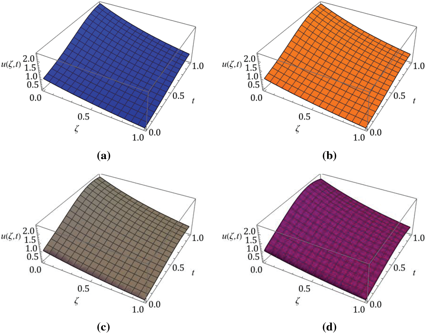
Figure 1: Nature of q-HATM solution Eq. (29) on the subject of ℏ=−1, n=1, and additionally with distinct values of α is presented in 3D graphs. (a) α=1, (b) α=0.9, (c) α=0.8, (d) α=0.7

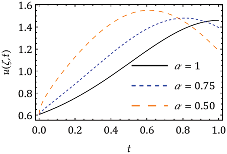
Figure 2: Response of solution u(ζ,t) by q-HATM with regard to t at ℏ=−1, ζ=0.5 and n=1 with varying α values

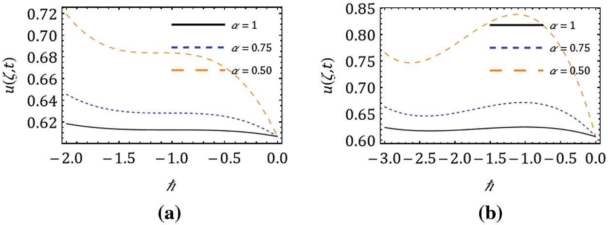
Figure 3: ℏ-curves for the solution u(ζ,t) with diverse values of α at ζ=0.5 and t=0.01 with different values of n. (a) n = 1, (b) n = 2

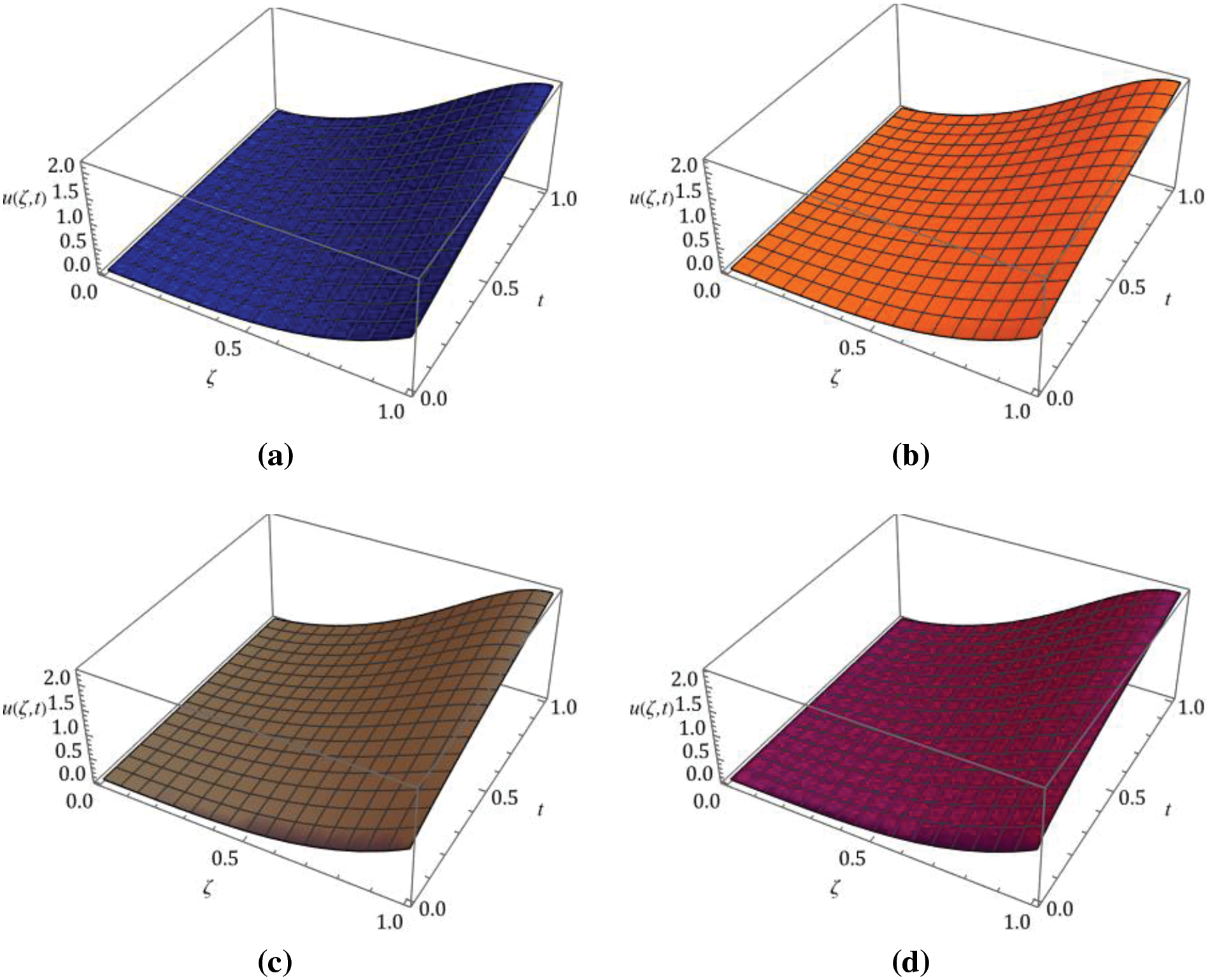
Figure 4: Behavior of the gained solution Eq. (38) by q-HATM at ℏ=−1, n=1 and with varying α values are plotted. (a) α=1, (b) α=0.9, (c) α=0.8 (d) α=0.7

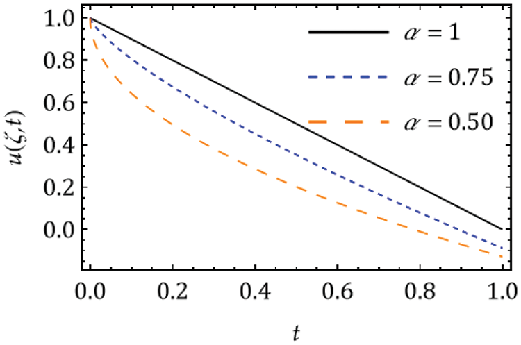
Figure 5: Solution u(ζ,t) vs. t at distinct α values are plotted when ℏ=−1, ζ=0.5, and n=1

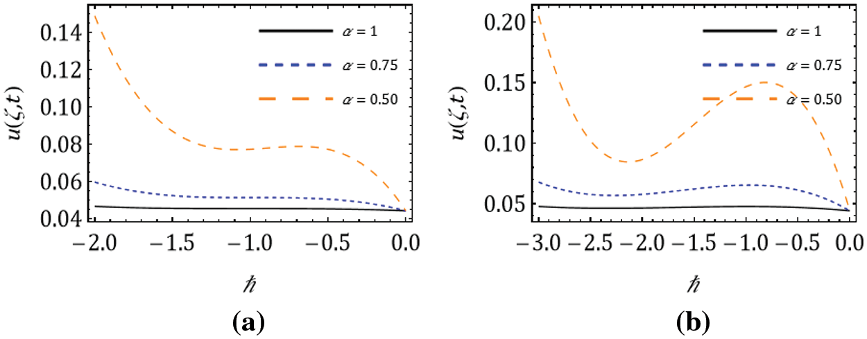
Figure 6: ℏ-curves plotted for Eq. (38) concerning ζ=0.5, t=0.001 with different α and n values. (a) n = 1, (b) n = 2

7  Conclusion

The necessity of the fractional-order derivative for the cancer tumor model is demonstrated. For this, the q-HATM method is implemented, which provides an influential solution for the fractional-order cancer model and achieves a solution in series form. Considered cases indicated that the net killing rate not only depends on time but also depends on the cancer cell concentration. The graphical presentation specifies that the concerned model depends on arbitrary order and parameters. This method is straightforward and efficient and can be enlarged to include numerous fractional-order models. In particular, the projected method helps to analyze and predict human disease growth and evaluate the physical and biological models. This study recommends framing fractional differential equations, which are crucial for describing how cancers spread and interact with one another, and using a cancer vaccination strategy, which can give significant changes in disease control in the early stages.

Acknowledgement: The Prince Sattam bin Abdulaziz University in Saudi Arabia is supporting this research under Project Number (PSAU/2024/01/99519). The authors also appreciate the insightful comments from anonymous reviewers, which have greatly improved this manuscript.

Funding Statement: Prince Sattam bin Abdulaziz University in Saudi Arabia supported this research under Project Number PSAU/2024/01/99519.

Author Contributions: The authors declare their contribution to the article as follows: study conception and design: Daasara Keshavamurthy Archana, Doddabhadrappla Gowda Prakasha; analysis and interpretation of results: Daasara Keshavamurthy Archana, Pundikala Veeresha; validation and supervision: Doddabhadrappla Gowda Prakasha, Kottakkaran Sooppy Nisar; draft manuscript preparation: Daasara Keshavamurthy Archana, Doddabhadrappla Gowda Prakasha, Pundikala Veeresha, Kottakkaran Sooppy Nisar. All authors reviewed the results and approved the final version of the manuscript.

Availability of Data and Materials: Since no datasets were created or examined during the current study, data sharing is not applicable.

Ethics Approval: Not applicable.

Conflicts of Interest: The authors declare that they have no conflicts of interest to report regarding the present study.

References

1. Tarasov VE. Fractional vector calculus and fractional Maxwell’s equations. Ann Phys. 2008;323(11): 2756–78. doi:10.1016/j.aop.2008.04.005. [Google Scholar] [CrossRef]

2. Cruz-Duarte JM, Rosales-Garcia J, Correa-Cely CR, Garcia-Perez A, Avina-Cervantes JG. A closed form expression for the Gaussian-based Caputo-Fabrizio fractional derivative for signal processing applications. Commun Non-Linear Sci Numer Simul. 2018;61(1):138–48. doi:10.1016/j.cnsns.2018.01.020. [Google Scholar] [CrossRef]

3. Tripathi D. Peristaltic transport of a viscoelastic fluid in a channel. Acta Astronaut. Apr. 2011;68(7):1379–85. doi:10.1016/j.actaastro.2010.09.012. [Google Scholar] [CrossRef]

4. Baleanu D, Wu G, Zeng S. Chaos analysis and asymptotic stability of generalized Caputo fractional differential equations. Chaos Solitons Fractals. 2017;102:99–105. doi:10.1016/j.chaos.2017.02.007. [Google Scholar] [CrossRef]

5. Sweilam NH, Abou Hasan MM, Baleanu D. New studies for general fractional financial models of awareness and trial advertising decisions. Chaos Solitons Fractals. 2017;104(3):772–84. doi:10.1016/j.chaos.2017.09.013. [Google Scholar] [CrossRef]

6. Bulut H, Sulaiman TA, Baskonus HM, Rezazadeh H, Eslami M, Mirzazadeh M. Optical solitons and other solutions to the conformable space-time fractional Fokas-Lenells equation. Optik. 2018;172(1):20–7. doi:10.1016/j.ijleo.2018.06.108. [Google Scholar] [CrossRef]

7. Liu DY, Gibaru O, Perruquetti W, Laleg-Kirati TM. Fractional order differentiation by integration and error analysis in noisy environment. IEEE Trans Autom Control. 2015;60(11):2945–60. doi:10.1109/TAC.2015.2417852. [Google Scholar] [CrossRef]

8. Veeresha P, Prakasha DG, Singh J, Khan I, Kumar D. Analytical approach for fractional extended Fisher-Kolmogorov equation with Mittag-Leffler kernel. Adv Differ Equ. 2020;2020(1):174. doi:10.1186/s13662-020-02617-w. [Google Scholar] [CrossRef]

9. Kumar CVD, Prakasha DG, Veeresha P, Kapoor M. A homotopy-based computational scheme for two-dimensional fractional cable equation. Mod Phys Lett B. 2024;6(2):2450292. doi:10.1142/S0217984924502920. [Google Scholar] [CrossRef]

10. Alatwi A, Bakeer A, Zaid S, Atawi I, Albalawi H, Kassem A. Intelligent fractional-order controller for SMES systems in renewable energy-based microgrid. Comput Model Eng Sci. 2024;140(2):1807–30. doi:10.32604/cmes.2024.048521. [Google Scholar] [CrossRef]

11. Agarwal P, Choi J. Fractional calculus operators and their image formulas. J Korean Math Soc. 2016;53(5):1183–210. doi:10.4134/JKMS.j150458. [Google Scholar] [CrossRef]

12. Drapaca CS, Sivaloganathan S. A fractional model of continuum mechanics. J Elast. 2012;107(2):105–23. doi:10.1007/s10659-011-9346-1. [Google Scholar] [CrossRef]

13. Shrahili M, Dubey RS, Shafay A. Inclusion of fading memory to Banister model of changes in physical condition. Discrete Cont Dyn-S. 2020;13(3):881–8. doi:10.3934/dcdss.2020051. [Google Scholar] [CrossRef]

14. Agarwal P, Baleanu D, Chen Y, Momani S, Machado JAT. Fractional calculus. In: Springer proceedings in mathematics & statistics, 2019; Springer: Singapore, vol. 303. doi:10.1007/978-981-15-0430-3. [Google Scholar] [CrossRef]

15. Arshad S, Sohail A, Javed S. Dynamical study of fractional order tumor model. Int J Comput Methods. 2015;12(5):1550032. doi:10.1142/S0219876215500322. [Google Scholar] [CrossRef]

16. Rihan FA, Abdel Rahman DH, Lakshmanan S, Alkhajeh AS. A time delay model of tumor-immune system interactions: global dynamics, parameter estimation, sensitivity analysis. Appl Math Comput. 2014;232(11):606–23. doi:10.1016/j.amc.2014.01.111. [Google Scholar] [CrossRef]

17. Kumar S, Kumar A, Samet B, Gómez-Aguilar JF, Osman MS. A chaos study of tumor and effector cells in fractional tumor-immune model for cancer treatment. Chaos Solitons Fractals. 2020;141(2):110321. doi:10.1016/j.chaos.2020.110321. [Google Scholar] [CrossRef]

18. Naik PA, Zu J, Naik M. Stability analysis of a fractional-order cancer model with chaotic dynamics. Int J Biomath. 2021;14(6):2150046. doi:10.1142/S1793524521500467. [Google Scholar] [CrossRef]

19. Gandhi H, Tomar A, Singh D. A predicted mathematical cancer tumor growth model of brain and its analytical solution by reduced differential transform method. In: Proceedings of International Conference on Trends in Computational and Cognitive Engineering, 2021; Singapore: Springer; p. 203–13. doi:10.1007/978-981-15-5414-8_17. [Google Scholar] [CrossRef]

20. Sweilam N, Al-Mekhlafi S, Ahmed A, Alsheri A, Abo-Eldahab E. Numerical treatments for crossover cancer model of hybrid variable-order fractional derivatives. Comput Model Eng Sci. 2024;140(2):1619–45. doi:10.32604/cmes.2024.047896. [Google Scholar] [CrossRef]

21. Farman M, Akgül A, Ahmad A, Imtiaz S. Analysis and dynamical behavior of fractional-order cancer model with vaccine strategy. Math Methods Appl Sci. 2020;43(7):4871–82. doi:10.1002/mma.6240. [Google Scholar] [CrossRef]

22. Panchal MM, Patel HS. Mathematical modelling and analysis of system of tumor-immune interaction by differential transform method. Solid State Technol. 2020;63(6):22591–8. [Google Scholar]

23. Ndenda JP, Njagarah JBH, Shaw S. Role of immunotherapy in tumor-immune interaction: perspectives from fractional-order modelling and sensitivity analysis. Chaos Solitons Fractals. 2021;148(1–2):111036. doi:10.1016/j.chaos.2021.111036. [Google Scholar] [CrossRef]

24. Korpinar Z, Inc M, Hınçal E, Baleanu D. Residual power series algorithm for fractional cancer tumor models. Alex Eng J. 2020;59(3):1405–12. doi:10.1016/j.aej.2020.03.044. [Google Scholar] [CrossRef]

25. Ali Dokuyucu M, Celik E, Bulut H, Baskonus HM. Cancer treatment model with the Caputo-Fabrizio fractional derivative. Eur Phys J Plus. 2018;133(3):92. doi:10.1140/epjp/i2018-11950-y. [Google Scholar] [CrossRef]

26. Saadeh R, Qazza A, Amawi K. A new approach using integral transform to solve cancer models. Fractal Fract. 2022;6(9):490. doi:10.3390/fractalfract6090490. [Google Scholar] [CrossRef]

27. Abaid Ur Rehman M, Ahmad J, Hassan A, Awrejcewicz J, Pawlowski W, Karamti H, et al. The dynamics of a fractional-order mathematical model of cancer tumor disease. Symmetry. 2022;14(8):1694. doi:10.3390/sym14081694. [Google Scholar] [CrossRef]

28. Padder A, Almutairi L, Qureshi S, Soomro A, Afroz A, Hincal E, et al. Dynamical analysis of generalized tumor model with caputo fractional-order derivative. Fractal Fract. 2023;7(3):258. doi:10.3390/fractalfract7030258. [Google Scholar] [CrossRef]

29. Burgess PK, Kulesa PM, Murray JD, Alvord ECJr. The interaction of growth rates and diffusion coefficients in a three-dimensional mathematical model of gliomas. J Neuropathol Exp Neurol. 1997;56(6):704–13. doi:10.1097/00005072-199706000-00008. [Google Scholar] [CrossRef]

30. Moyo S, Leach P. Symmetry methods applied to a mathematical model of a tumor of the brain. In: Proceedings of Institute of Mathematics of NAS of Ukraine, 2004; vol. 50, p. 204–10. [Google Scholar]

31. Odibat Z. On Legendre polynomial approximation with the VIM or HAM for numerical treatment of non-linear fractional differential equations. J Comput Appl Math. 2011;235(9):2956–68. doi:10.1016/j.cam.2010.12.013. [Google Scholar] [CrossRef]

32. Iyiola OS, Zaman FD. A fractional diffusion equation model for cancer tumor. AIP Adv. 2014;4(10):107121. doi:10.1063/1.4898331. [Google Scholar] [CrossRef]

33. Arqub OA, El-Ajou A. Solution of the fractional epidemic model by homotopy analysis method. J King Saud Univ-Sci. 2013;25(1):73–81. doi:10.1016/j.jksus.2012.01.003. [Google Scholar] [CrossRef]

34. Abdl-Rahim HR, Zayed M, Ismail GM. Analytical study of fractional epidemic model via natural transform homotopy analysis method. Symmetry. 2022;14(8):1695. doi:10.3390/sym14081695. [Google Scholar] [CrossRef]

35. Veeresha P, Ilhan E, Prakasha DG, Baskonus HM, Gao W. A new numerical investigation of fractional order susceptible-infected-recovered epidemic model of childhood disease. Alex Eng J. 2022;61(2):1747–56. doi:10.1016/j.aej.2021.07.015. [Google Scholar] [CrossRef]

36. Prakasha DG, Malagi NS, Veeresha P, Prasannakumara BC. An efficient computational technique for time-fractional Kaup-Kupershmidt equation. Numer Methods Partial Differ Equ. 2021;37(2):1299–316. doi:10.1002/num.22580. [Google Scholar] [CrossRef]

37. Prakash A, Goyal M, Gupta S. q-homotopy analysis method for fractional Bloch model arising in nuclear magnetic resonance via the Laplace transform. Indian J Phys. 2020;94(4):507–20. doi:10.1007/s12648-019-01487-7. [Google Scholar] [CrossRef]

38. Veeresha P, Malagi NS, Prakasha DG, Baskonus HM. An efficient technique to analyze the fractional model of vector-borne diseases. Phys Scr. 2022;97(5):054004. doi:10.1088/1402-4896/ac607b. [Google Scholar] [CrossRef]

39. Veeresha P, Prakasha DG, Baleanu D. An efficient technique for fractional coupled system arisen in magnetothermoelasticity with rotation using Mittag-Leffler kernel. J Comput Nonlinear Dyn. 2020;16(1):011002. doi:10.1115/1.4048577. [Google Scholar] [CrossRef]

40. Seddek LF, El-Zahar ER, Chung JD, Shah NA. A novel approach to solving fractional-order Kolmogorov and Rosenau-Hyman models through the q-homotopy analysis transform method. Mathematics. 2023;11(6):1321. doi:10.3390/math11061321. [Google Scholar] [CrossRef]

41. Yasmin H, Alshehry AS, Saeed AM, Shah R, Nonlaopon K. Application of the q-homotopy analysis transform method to fractional-order Kolmogorov and Rosenau-Hyman models within the Atangana-Baleanu operator. Symmetry. 2023;15(3):671. doi:10.3390/sym15030671. [Google Scholar] [CrossRef]

42. Podlubny I. Fractional differential equations, 1999; New York: Academic Press. [Google Scholar]

43. Caputo M. Elasticità e dissipazione. Bologna: Zanichelli; 1969. [Google Scholar]

44. Miller KS, Ross B. An introduction to the fractional calculus and fractional differential equations. New York: Wiley; 1993. [Google Scholar]

45. Magreñán AA. A new tool to study real dynamics: the convergence plane. Appl Math Comput. 2014;248(4):215–24. doi:10.1016/j.amc.2014.09.061. [Google Scholar] [CrossRef]

46. Argyros IK, Convergence and applications of Newton-type iterations. New York: Springer; 2008. doi:10.1007/978-0-387-72743-1. [Google Scholar] [CrossRef]