
 Submit a Paper
 Propose a Special lssue
 Open Access
ARTICLE
Modeling the Dynamics of Tuberculosis with Vaccination, Treatment, and Environmental Impact: Fractional Order Modeling
1 Faculty of Natural and Agricultural Sciences, University of the Free State, Bleomfontein, 9300, South Africa
2 Department of Basic Sciences, Princess Sumaya University for Technology, Amman, 11941, Jordan
3 Department of Clinical Laboratory Sciences, College of Applied Medical Science, King Khalid University, Abha, 62529, Saudi Arabia
4 Mathematical Sciences Department, College of Applied Sciences, Umm Al-Qura University, Makkah, 24381, Saudi Arabia
5 Department of Mathematics, Faculty of Science, King Abdulaziz University, P.O. Box 80203, Jeddah, 21589, Saudi Arabia
* Corresponding Author: Muhammad Altaf Khan. Email:
(This article belongs to the Special Issue: Analytical and Numerical Solution of the Fractional Differential Equation)
Computer Modeling in Engineering & Sciences 2024, 141(2), 1365-1394. https://doi.org/10.32604/cmes.2024.053681
Received 07 May 2024; Accepted 18 July 2024; Issue published 27 September 2024
 View Full Text
 Download PDF
Abstract
A mathematical model is designed to investigate Tuberculosis (TB) disease under the vaccination, treatment, and environmental impact with real cases. First, we introduce the model formulation in non-integer order derivative and then, extend the model into fractional order derivative. The fractional system’s existence, uniqueness, and other relevant properties are shown. Then, we study the stability analysis of the equilibrium points. The disease-free equilibrium (DFE) is locally asymptotically stable (LAS) when . Further, we show the global asymptotical stability (GAS) of the endemic equilibrium (EE) for and for . The existence of bifurcation analysis in the model is investigated, and it is shown the system possesses the forward bifurcation phenomenon. Sensitivity analysis has been performed to determine the sensitive parameters that impact . We consider the real TB statistics from Khyber Pakhtunkhwa in Pakistan and parameterized the model. The computed basic reproduction number obtained using the real cases is . Various numerical results regarding disease elimination of the sensitive parameters are shown graphically.Keywords
A Mycobacterium tuberculosis (MTB) infection is the reason for tuberculosis (TB), a persistent contagious disease that frequently spreads through the air in the form of droplets [1]. Pulmonary tuberculosis is the name given to TB that mostly affects the lungs, however, it can affect any organ in the body [2]. Before the COVID-19 pandemic in 2019, TB ranked as the world’s 13th most common cause of mortality and the primary cause of death from single-source infections. Even though TB prevention and mitigation have come a long way over the last 20 years, 10.6 million new cases of the disease were reported globally in 2021. Based on estimates, Pakistan ranked fifth among B high-burden nations globally, accounting for
Several recent mathematical studies have been conducted on TB dynamics in the past. For example, the authors in [5] introduced a mathematical formulation for TB dynamics and discussed the disease trends in India and other nations. The work in [6], provided the development of the age structure modeling of TB controlling under dots. Further, different case studies have investigated related to TB cures in different areas of the world. In [7], the authors conducted a study, to examine the TB dynamics incorporated by the features of slow and fast progression within the SEIR (Susceptible, Exposed, Infected, Recovered) model. The recurrence features in the TB model formulation have been done by [8], where the authors considered an XL
Vaccination is considered a powerful tool for the prevention and control of diseases. The authors in [21] studied the COVID-19 spread in China with vaccination in some percentage. The authors in [22] studied the model with the Omicron strain and the Delta variant strain. To prevent TB disease, administer the BCG vaccine, which is made from a suspension of attenuated Bacillus bovis. It boosts macrophage action, enhances tumor cell killing, activates T lymphocytes, and improves cellular immunity. The two French scientists, Calmette and Guerin, are the first to develop it [23,24]. For a long time, it was considered that the vaccine BCG does not protect against the mycobacterium tuberculosis infection, however, it protects against progression of the active disease [25]. A vaccination model in [26] is formulated to study TB infection with relapse incomplete treatment, and slow and past progression.
Scientists and researchers are always exploring ways to find the best possible treatment against the disease for it curtail. Presently, the treatment available for TB is drug treatment. The TB treatment follows five principles and with many constraints, treatment for an individual frequently falls short of the intended outcomes. The incomplete treatment causes some of the infected people to have drug-resistant infections [19]. The latent individuals, as a control strategy to design an optimal control problem for TB, have been studied in [27]. Various studies indicate the survival of the TB bacteria outside the host in favorable conditions for a long time and even alcohol with 75% cannot be able to vanish it. Healthy individuals can easily be infected with the pathogens in the environment that is available to live freely. Thus, the concept of environmental study in TB modeling has been incorporated by many researchers [28]. The contaminated environment effect includes handkerchiefs, doorknobs, towels, and toys used by infected individuals. The authors conducted research on TB with environmental class in their mathematical modeling in China [29]. Some more related work in applied mathematics area are provided here in the work [30,31].
An expanded form of integer-order calculus is called fractional calculus. In the last few decades, it has been widely applied in various scientific and technological fields, such as electronic circuit analysis, control theory, heat transfer, and fluid dynamics [32]. The fractional derivative is primarily used because it incorporates memory, a feature shared by the majority of biological systems. Moreover, the fractional order derivative has a nonlocal characteristic. Additionally, the dynamical systems’ stability zone is expanded by fractional-order derivatives. It has been heavily utilized in the past several years to address numerous biological issues. The difficulties are modeled using differential equations of fractional order. In this connection, we may cite various research in which non-integer derivatives are considered to simulate and examine the transmission of different types of illnesses other than TB (see [33,34]). For example, a fractional study to examine TB disease has been considered in [35]. A mathematical model of TB in Caputo-Fabrizio derivative is explored in [36]. The COVID-19 mathematical study in different fractional kernels is given in [37]. A Zika virus model under fractional differential equation modeling is studied in [38]. There is more related research on fractional derivatives, see [39–42].
We design a mathematical model in the present analysis for tuberculosis infection with vaccination, environmental contamination, and therapies that significantly influence the TB disease’s dynamics. In the previous works mentioned above none of us used the concept of fractional derivative with real data of KP, in Pakistan to study TB, with vaccination, environmental impacts, and treatment. We considered a perfect vaccination and provided the results when there was an increase in vaccine and less waning rate of vaccine. We use real data and provide a more detailed analysis of the model with qualitative and numerical results. The rest of the paper has been organized in detail section-wise as follows: The basic definitions and the construction of the mathematical model are given in Section 2. The fundamental analysis of the model and its existence and uniqueness is shown in Section 3 while bifurcation and the local stability analysis are discussed in Section 4. Section 5studies the global stability analysis of the proposed model. Parameters estimation is shown in Section 6 while the detailed numerical results are given in Section 7. Results are summarized finally in Section 8.
2 Model Construction and Basic of Fractional Formulae
We shall provide some important formulae that will be used in the modeling of the problem. We follow the definitions from [32,43].
Definition 1. A Caputo derivative of order
Definition 2. We can define the fractional Riemann–Liouville of the function
where
The present section formulates a mathematical model for tuberculosis infection, with treatment, vaccination, and environmental contamination. The model consists of seven classes where the population of humans is distributed among six different categories, such as susceptible people,
where the initial conditions subject to the system (3) are given by
In the TB system (3), the parameters
We shall carry out some important results regarding the fractional system (5) in the present portion.
Theorem 1. All the associated solutions to the system (5) are uniformly bounded and nonnegative.
Proof. It follows from the model (5) we get
So, it follows from the work given in [44] that all the solution will remain always in
Now consider the result from [45], we obtain
where
Again using the result from [45], we have
Hence,
■
The existence of a unique solution is given in the theorem below.
Theorem 2. There exists a unique solution associated to the system (5).
Proof. Denote
where
Denoting
where
4 Analysis of the Equilibrium Points
First, we obtain the disease-free equilibrium point of the model (5) in the following by solving the equations of the model (5) at a steady state by setting:
We get the following equilibrium point called the disease-free equilibrium is given by
where
To study the analysis of the equilibrium points, first, we need to obtain the expression for the basic reproduction number
Further, we have the following matrices:
Using the concept of spectral radius of
where
We give the comparison of the basic reproduction number
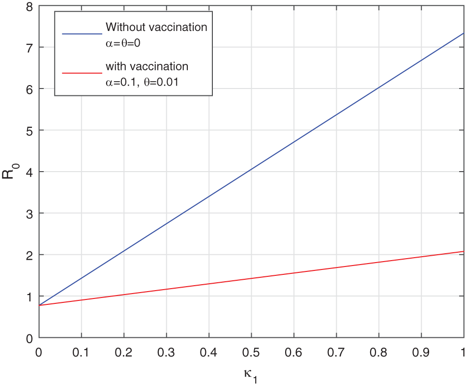
Figure 1: Comparison of
Endemic Equilibria
The finding of the expression of the endemic equilibria is important in disease models as it determines the number of possible equilibrium points in the presence of infection. Further, the existence of unique or multiple endemic equilibria determines the possibility of the bifurcation which may be of different types, such as forward or backward. We use the notation
where
Now, putting the above equations into
and then simplifying, we obtain the following:
where
Here,
Theorem 3. The fractional system (5) at
Proof. At
The characteristics equation related to J is
where
where
and
4.1 Backward Bifurcation Analysis
We present the backward bifurcation analysis of the model (5) when
where
and
According to [48], the coefficients are
need to be computed using the second-order partial derivatives obtained at
and
where
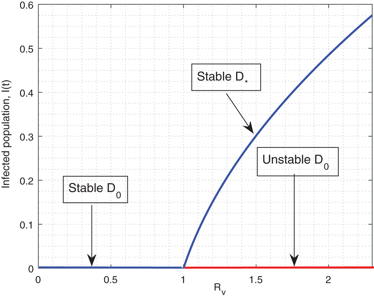
Figure 2: The plot describes the existence of the forward bifurcation in the model (3)
We use the Lemma in the proof of global stability.
Lemma 1. [49]. Consider that a continuous and derivable function
Theorem 4. The fractional system (5) at
Proof. We consider the following Lyapunov function:
where the positive constants
Now, consider the values assigned to the constants
It follows that
5.1 Global Stability Endemic Equilibrium (EE)
The following assumptions are made based on steady-state
Theorem 5. The infected equilibrium
Proof. Let us consider the Lyapunov function in the structure given below:
where
where
Computing the terms on the right side of Eq. (13) one by one below:
We submit the above into Eq. (12) and simplifying, we obtain,
Here, the arithmetic mean is greater or equal to the geometric mean, so we get,
If
■
The estimation of the parameters of the model (5) will be investigated for
i) Create the objective function that measures how much the real and projected values vary from one another. The stated designed function is the sum of squared residuals between the model’s forecast and the corresponding real data cases.
ii) First, provide the initial values of the parameters that need estimations. It might be an initial guess or a prior knowledge base.
iii) Using the initial values of the parameters shown in step (ii), the model is simulated to obtain the predictions of the model.
iv) Applying the “lsqcurvefit” optimization technique to see whether the objective function can be minimized.
v) Setting convergence criteria to end the process of iterative estimating. It is based on reaching a predetermined threshold for the relevant objective function, an appropriate number of iterations, or the smallest modification in parameter estimations.
vi) Set the original parameter estimations back to repeat steps (i–v) until an acceptable agreement across the model simulation and the actual data is attained if the estimated parameter values do not fulfill the convergence condition or do not match the real data curve sufficiently.
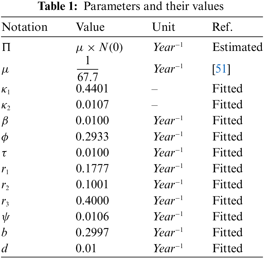
The model in the absence of vaccination provides a reasonable fitting which is shown in Fig. 3 while the obtained fitted/estimated parameters are shown briefly in Table 1. For the parameter values listed in Table 1, we computed
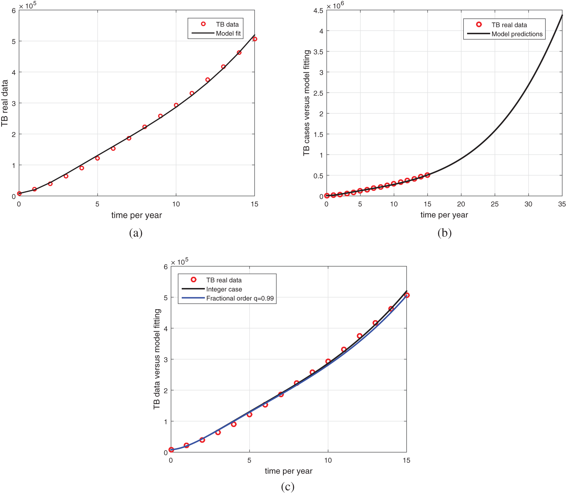
Figure 3: Model fitting with real data. The circle shows real TB data while the bold line is the model solution. (a) model vs. data fitting (b) data vs. model long-time predictions (c) data vs. fractional model
6.1.1 Local Sensitivity Analysis
Here, we study the sensitivity analysis of the parameters involved in
where
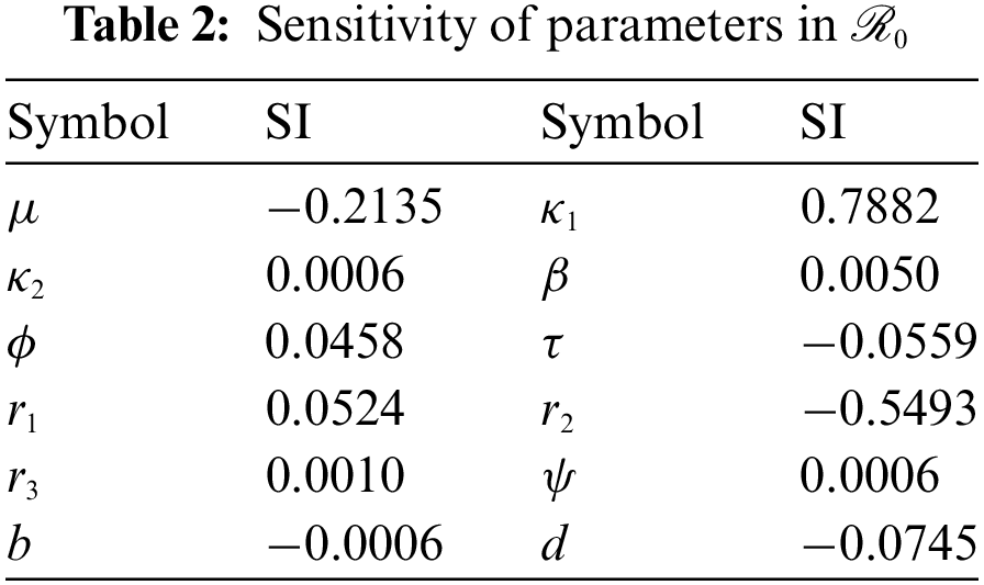
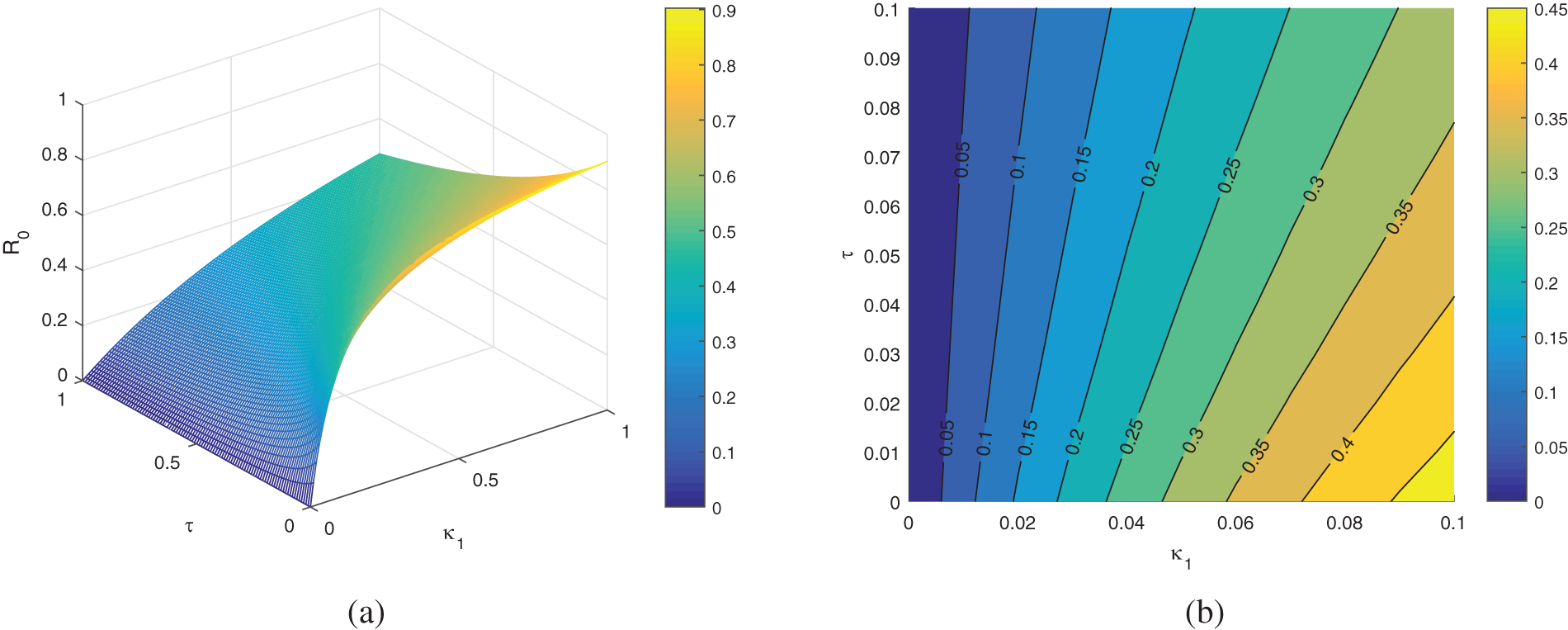
Figure 4: The plot represents the parameters
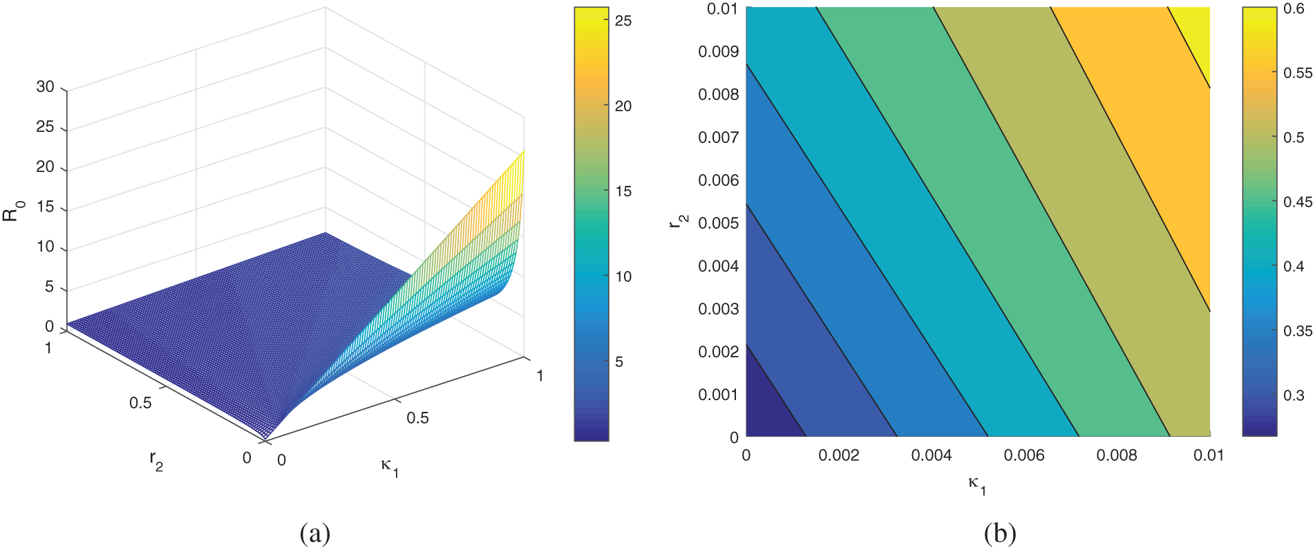
Figure 5: The plot represents the parameters
6.1.2 Global Sensitivity Analysis
This section studies the sensitivity and uncertainty of the basic reproduction
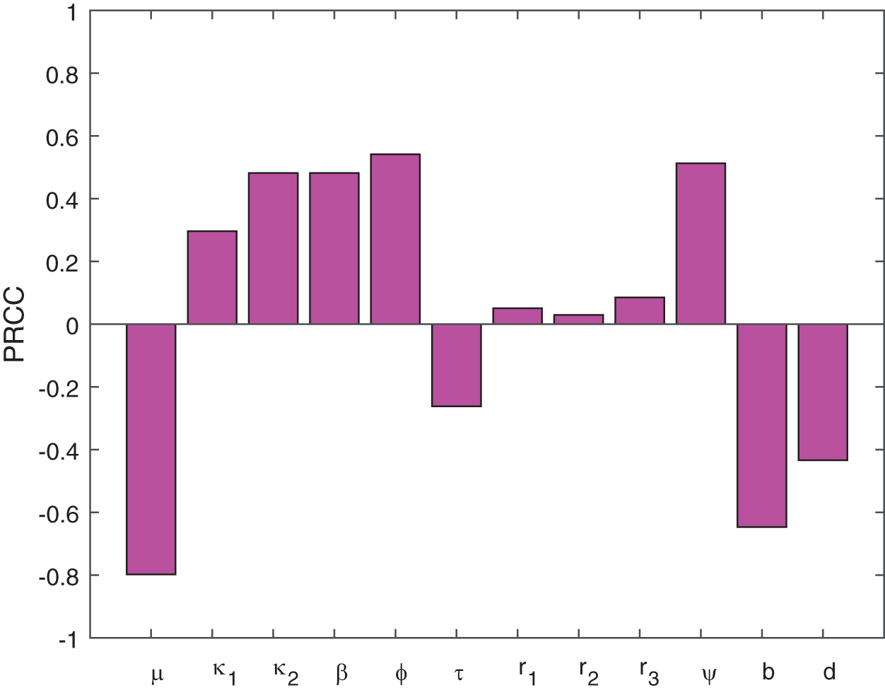
Figure 6: The plot indicates the sensitivity of
We perform the numerical simulation in the present section by considering the parameter values shown in Table 1. The model (5) is solved numerically by the method explained in [46,56]. According to the nature of the data, we consider the units in simulation per year. We present graphical results for the fractional model (5) under different fractional orders. Figs. 7 and 8 show the dynamics of the model using different fractional order

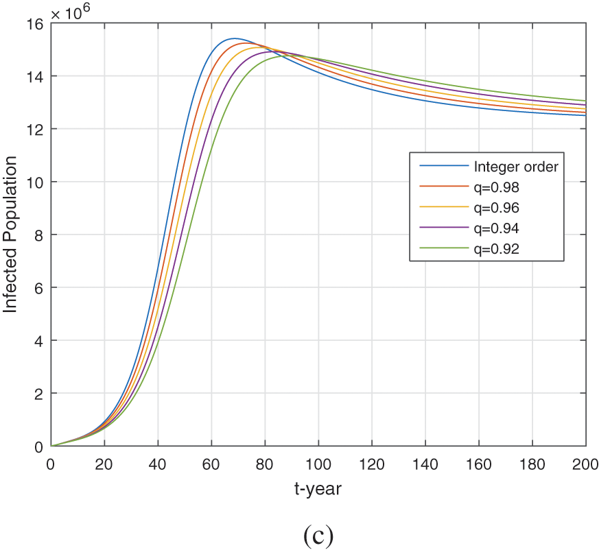
Figure 7: Numerical simulation of the healthy, exposed, and infected compartments (a–c) respectively for different fractional order
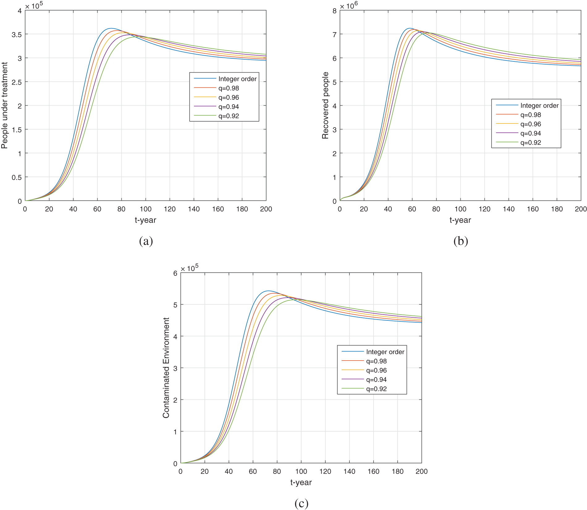
Figure 8: Numerical simulation of the treated, recovered and contaminated environmental compartments (a–c) respectively for different fractional order
We see from Fig. 9 the impact of the
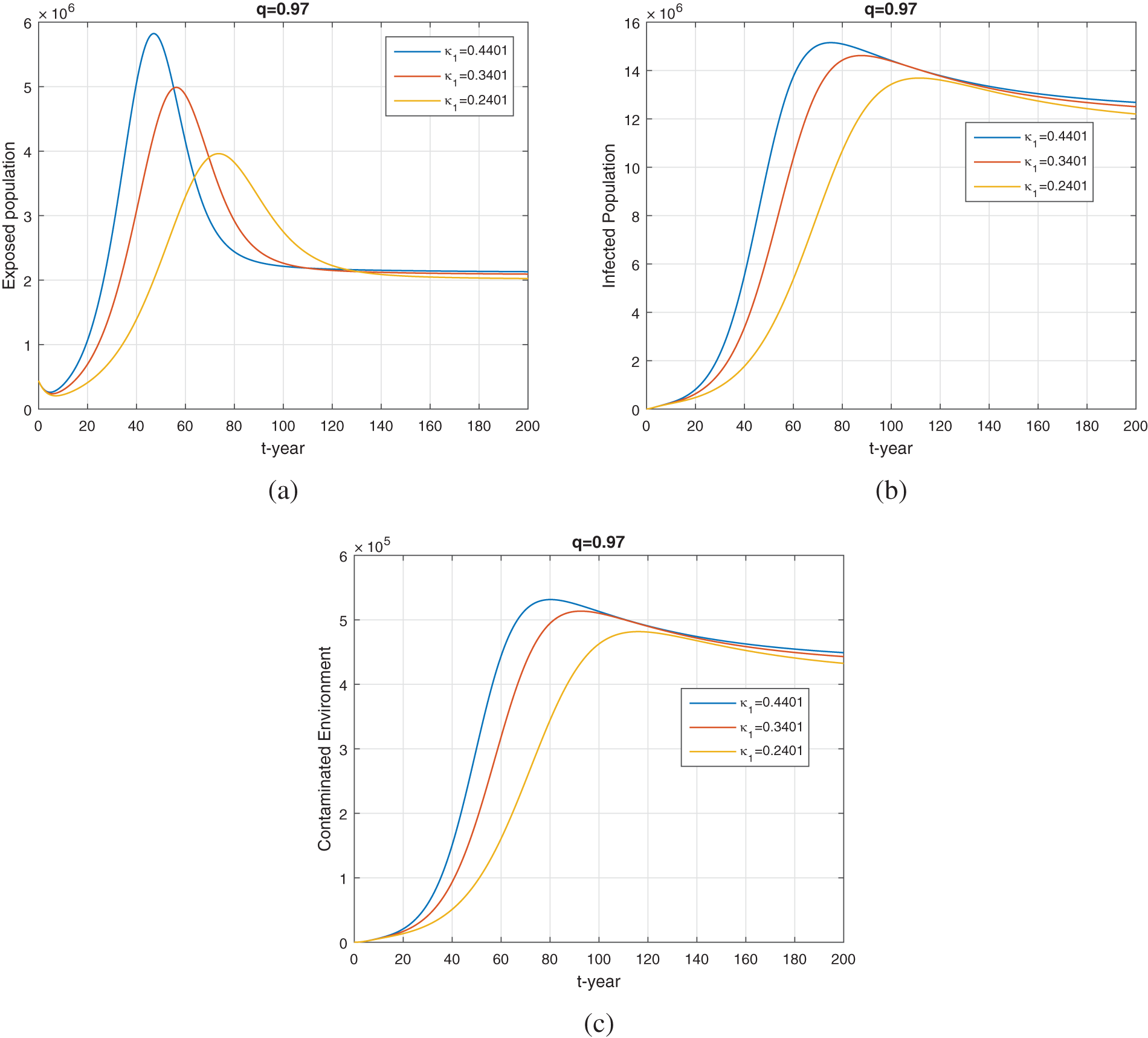
Figure 9: The plot shows the dynamics of exposed, infected and environmental population for various values of
Fig. 10 represents the comparison of vaccination vs. no vaccination on the dynamics of exposed, infected, and environmental populations. It can be seen that the vaccine impacts greatly disease dynamics and reduces future cases in society. When increasing the vaccine rate
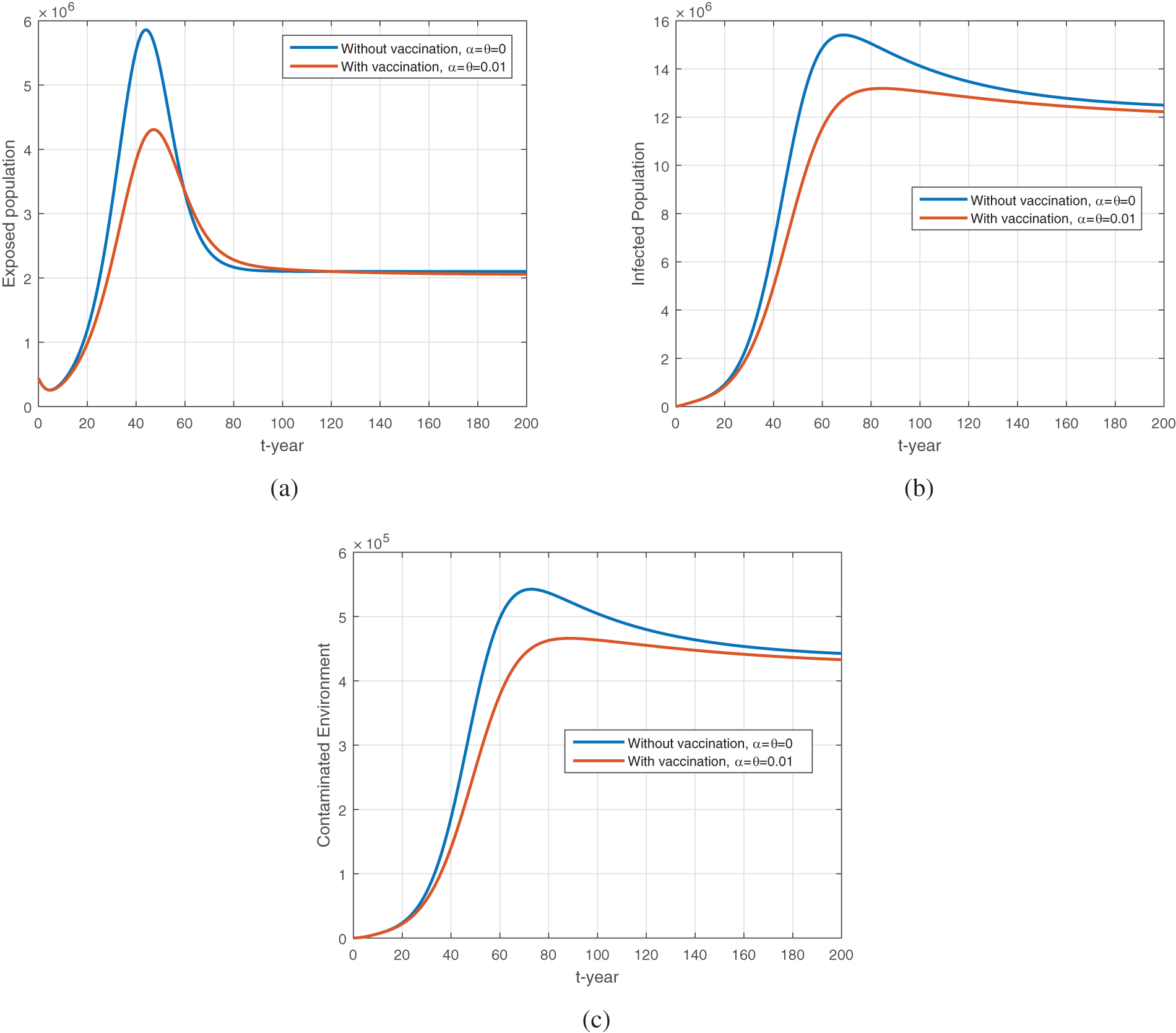
Figure 10: The plot shows the dynamics of exposed, infected and environmental population with and without vaccination. (a) to (c) represent the exposed, infected, and environmental population
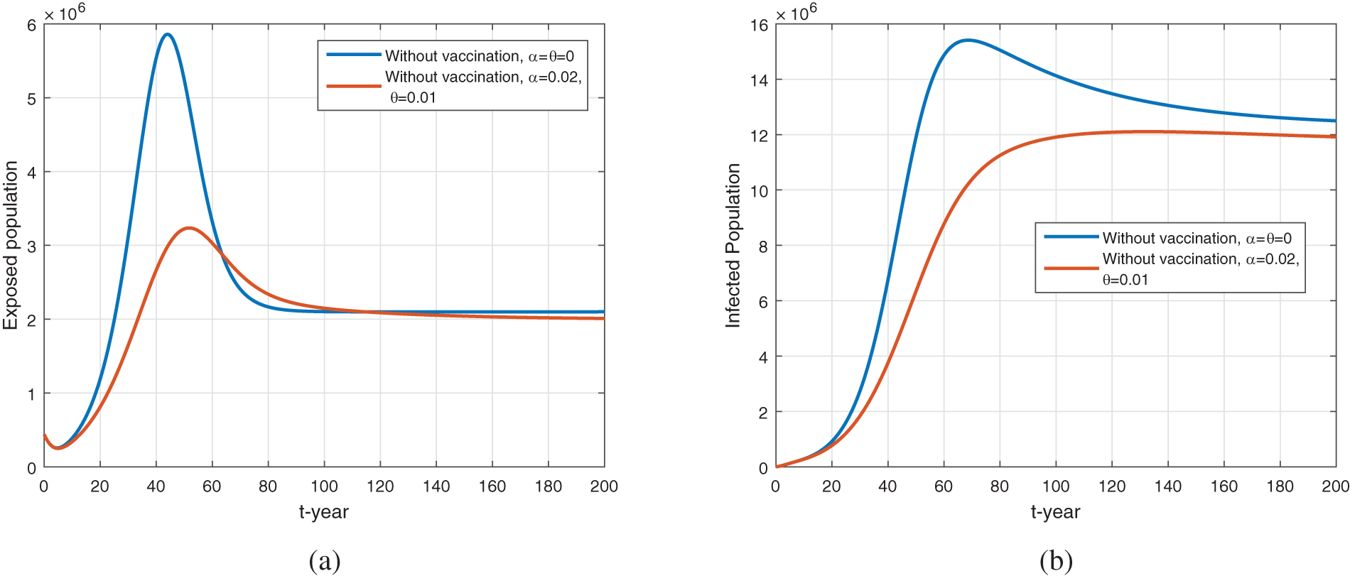
Figure 11: The plot shows the dynamics of exposed and infected population for
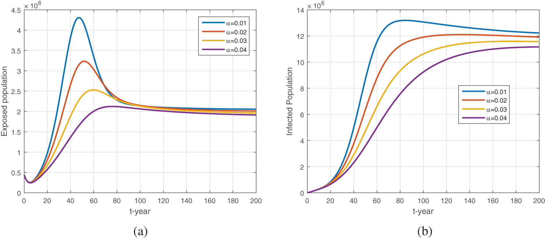
Figure 12: The plot shows the dynamics of exposed and infected populations with the variation in
We show the results for the treatment parameter
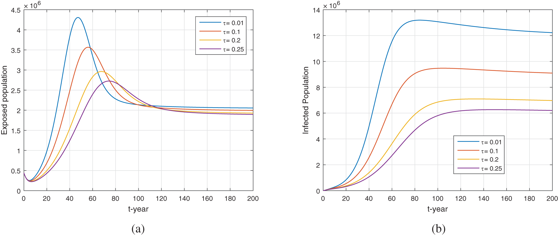
Figure 13: The treatment impact on the dynamics of exposed and infected population when varying
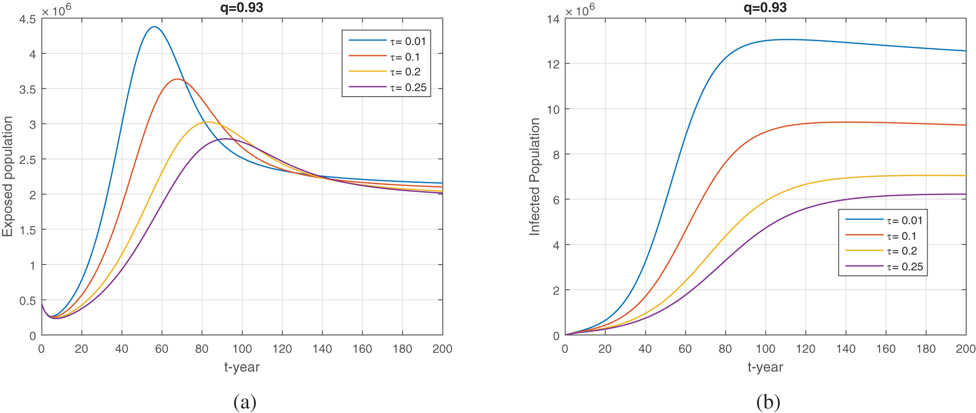
Figure 14: The treatment impact on the dynamics of exposed and infected population when varying
In this study, we investigated tuberculosis infection with treatment, vaccination, and environmental impact using non-integer order derivatives. The basic modeling is done initially in integer case and later the model is extended to non-integer order based on the definition of Caputo. First, the formulation of the model has been obtained and discussed in detail. Then, we extended the model into a fractional order differential equation using the concept of Caputo derivative. The existence and uniqueness of the fractional model have been obtained. The stability of the equilibrium points is obtained and discussed based on
We considered the real data of TB in Khyber Pakhtunkhwa in Pakistan and experimented using the nonlinear least square method. The estimated parameters obtained from the experiment that provided reasonable fitting to the data have been used in numerical simulation and obtained graphical results regarding disease elimination. We observed that vaccinating more and more individuals and reducing the contact between healthy and infected people can minimize well the future cases of TB in the country. The treatment provides important results regarding the disease control of TB in the country. Increasing the treatment for the long-term program, the number of TB cases has decreased significantly in the country. Vaccination impact on the disease has a significant impact on the TB cases in Pakistan. The results obtained in the numerical section show that vaccination has a great impact on the reduction of TB cases. So, vaccination, treatment, and controlling environmental contamination will significantly decrease TB cases in the country shortly.
The results obtained in the work are based on the formulation of the model with their parameters and the available data. The time domain considered for the data is per year which may have different impacts with other time units. The model results rely on the real data used and the accuracy is limited to the quality and quantitative data which is different from the other data used in the model. The demographic parameters may vary from region to region and thus will have different results. The environmental factors are also different from region to region and hence will impact the result.
Acknowledgement: The authors are thankful to the Deanship of Research and Graduate Studies, King Khalid University, Abha, Saudi Arabia, for financially supporting this work through the Large Research Group Project under Grant No. R.G.P.2/507/45.
Funding Statement: This work is supported by King Khalid University.
Author Contributions: Muhammad Altaf Khan, Mahmoud H. DarAssi, Irfan Ahmad; data collection: Noha Mohammad Seyam; Ebraheem Alzahrani; Muhammad Altaf Khan, analysis and interpretation of results: Muhammad Altaf Khan, Mahmoud H. DarAssi and Ebraheem Alzahrani; draft manuscript preparation: Muhammad Altaf Khan, Mahmoud H. DarAssi. All authors reviewed the results and approved the final version of the manuscript.
Availability of Data and Materials: The data used in the manuscript is available from the corresponding author on a reasonable request.
Ethics Approval: Not applicable.
Conflicts of Interest: The authors declare that they have no conflicts of interest to report regarding the present study.
References
1. Tuberculosis; 2023. Available from: https://www.who.int/news-room/fact-sheets/detail/tuberculosis. [Accessed 2023]. [Google Scholar]
2. George M. The challenge of culturally competent health care: applications for asthma. Heart & Lung. 2001;30(5):392–400. doi:10.1067/mhl.2001.118364. [Google Scholar] [PubMed] [CrossRef]
3. Pakistan. Tuberculosis. Available from: https://www.emro.who.int/pak/programmes/stop-tuberculosis.html. [Accessed 2023]. [Google Scholar]
4. World Health Organization. Available from: https://www.who.int/en/news-room/factsheets/detail/tuberculosis. [Accessed 2023]. [Google Scholar]
5. Waaler H, Geser A, Andersen S. The use of mathematical models in the study of the epidemiology of tuberculosis. Am J Public Health and the Nations Health. 1962;52(6):1002–13. doi:10.2105/AJPH.52.6.1002. [Google Scholar] [PubMed] [CrossRef]
6. Dye C, Garnett GP, Sleeman K, Williams BG. Prospects for worldwide tuberculosis control under the WHO DOTS strategy. Lancet. 1998;352(9144):1886–91. doi:10.1016/S0140-6736(98)03199-7. [Google Scholar] [PubMed] [CrossRef]
7. Song B, Castillo-Chavez C, Aparicio JP. Tuberculosis models with fast and slow dynamics: the role of close and casual contacts. Math Bio. 2002;180(1–2):187–205. doi:10.1016/S0025-5564(02)00112-8. [Google Scholar] [PubMed] [CrossRef]
8. Porco TC, Blower SM. Quantifying the intrinsic transmission dynamics of tuberculosis. Theor Popul Biol. 1998;54(2):117–32. doi:10.1006/tpbi.1998.1366. [Google Scholar] [PubMed] [CrossRef]
9. Bhunu C, Garira W, Mukandavire Z, Magombedze G. Modelling the effects of pre-exposure and post-exposure vaccines in tuberculosis control. J Theor Biol. 2008;254(3):633–49. doi:10.1016/j.jtbi.2008.06.023. [Google Scholar] [PubMed] [CrossRef]
10. Yang Y, Tang S, Xlaohong R, Zhao H, Guo C. Global stability and optimal control for a tuberculosis model with vaccination and treatment. Discrete Conti Dyn Syst Ser B. 2016;21(3):1–26. doi:10.3934/dcdsb. [Google Scholar] [CrossRef]
11. Ziv E, Daley CL, Blower S. Potential public health impact of new tuberculosis vaccines. Emerg Infect Dis. 2004;10(9):1529–35. doi:10.3201/eid1009.030921. [Google Scholar] [PubMed] [CrossRef]
12. Ren S. Global stability in a tuberculosis model of imperfect treatment with age-dependent latency and relapse. Math Biosci Eng. 2017;14(5&6):1337–60. doi:10.3934/mbe.2017069. [Google Scholar] [PubMed] [CrossRef]
13. Trauer JM, Denholm JT, McBryde ES. Construction of a mathematical model for tuberculosis transmission in highly endemic regions of the Asia-Pacific. J Theor Biol. 2014;358(33):74–84. doi:10.1016/j.jtbi.2014.05.023. [Google Scholar] [PubMed] [CrossRef]
14. Khan MA, Ullah S, Farooq M. A new fractional model for tuberculosis with relapse via Atangana-Baleanu derivative. Chaos Soliton Fract. 2018;116(2):227–38. doi:10.1016/j.chaos.2018.09.039. [Google Scholar] [CrossRef]
15. Bhunu C, Garira W, Mukandavire Z. Modeling HIV/AIDS and tuberculosis coinfection. Bull Math Biol. 2009;71(7):1745–80. doi:10.1007/s11538-009-9423-9. [Google Scholar] [PubMed] [CrossRef]
16. Guo ZK, Xiang H, Huo HF. Analysis of an age-structured tuberculosis model with treatment and relapse. J Math Biol. 2021;82(5):1–37. doi:10.1007/s00285-021-01595-1. [Google Scholar] [PubMed] [CrossRef]
17. Xue L, Jing S, Wang H. Evaluating strategies for tuberculosis to achieve the goals of WHO in China: a seasonal age-structured model study. Bull Math Biol. 2022;84(6):61. doi:10.1007/s11538-022-01019-1. [Google Scholar] [PubMed] [CrossRef]
18. Bowong S, Kurths J. Modeling and analysis of the transmission dynamics of tuberculosis without and with seasonality. Nonlin Dyn. 2012;67(3):2027–51. doi:10.1007/s11071-011-0127-y. [Google Scholar] [CrossRef]
19. Kang TL, Huo HF, Xiang H. Dynamics and optimal control of tuberculosis model with the combined effects of vaccination, treatment and contaminated environments. Math Biosci Eng. 2024;21(4):5308–34. doi:10.3934/mbe.2024234. [Google Scholar] [PubMed] [CrossRef]
20. Fatima B, Yavuz M, ur Rahman M, Al-Duais FS. Modeling the epidemic trend of middle eastern respiratory syndrome coronavirus with optimal control. Math Biosci Eng. 2023;20(7):11847–74. doi:10.3934/mbe.2023527. [Google Scholar] [PubMed] [CrossRef]
21. Li T, Guo Y. Modeling and optimal control of mutated COVID-19 (Delta strain) with imperfect vaccination. Chaos Soliton Fract. 2022;156(4):111825. doi:10.1016/j.chaos.2022.111825. [Google Scholar] [PubMed] [CrossRef]
22. Guo Y, Li T. Modeling the competitive transmission of the Omicron strain and Delta strain of COVID-19. J Math Anal Appl. 2023;526(2):127283. doi:10.1016/j.jmaa.2023.127283. [Google Scholar] [PubMed] [CrossRef]
23. Hawn TR, Day TA, Scriba TJ, Hatherill M, Hanekom WA, Evans TG, et al. Tuberculosis vaccines and prevention of infection. Microb Mol Biol Rev. 2014;78(4):650–71. doi:10.1128/MMBR.00021-14. [Google Scholar] [PubMed] [CrossRef]
24. Bin Sayeed MS, James SL, Abate D, Abate KH, Abay SM, Abbafati C, et al. Global, regional, and national incidence, prevalence, andyears lived with disability for 354 diseases and injuries for 195 countries and territories, 1990–2017: a systematicanalysis for the Global Burden of Disease Study 2017. Global Health Metrics. 2020;396(10258):1204–22. doi:10.1016/S0140-6736(18)32279-7. [Google Scholar] [CrossRef]
25. White PJ, Garnett GP. Mathematical modelling of the epidemiology of tuberculosis. In: Modelling parasite transmission and control. 2010. vol. 673, p. 127–40. doi:10.1007/978-1-4419-6064-1_9. [Google Scholar] [PubMed] [CrossRef]
26. Li Y, Liu X, Yuan Y, Li J, Wang L. Global analysis of tuberculosis dynamical model and optimal control strategies based on case data in the United States. Appl Math Comput. 2022;422:126983. [Google Scholar]
27. Jiang Q, Liu Z, Wang L, Tan R. A tuberculosis model with early and late latency, imperfect vaccination, and relapse: an application to China. Math Methods Appl Sci. 2023;46(9):10929–46. [Google Scholar]
28. Xu A, Wen ZX, Wang Y, Wang WB. Prediction of different interventions on the burden of drug-resistant tuberculosis in China: a dynamic modelling study. J Glob Antimicrob Resist. 2022;29:323–30. [Google Scholar] [PubMed]
29. Cai Y, Zhao S, Niu Y, Peng Z, Wang K, He D, et al. Modelling the effects of the contaminated environments on tuberculosis in Jiangsu. China J Theor Biol. 2021;508:110453. [Google Scholar] [PubMed]
30. Sk N, Mondal B, Thirthar AA, Alqudah MA, Abdeljawad T. Bistability and tristability in a deterministic prey-predator model: transitions and emergent patterns in its stochastic counterpart. Chaos Soliton Fract. 2023;176:114073. [Google Scholar]
31. Nyaberi H, Mutuku W, Malonza D, Gachigua G, Alworah G. An optimal control model for Coffee Berry Disease and Coffee Leaf Rust co-infection. J Math Anal Model. 2024;5(1):1–25. [Google Scholar]
32. Podlubny I. Fractional differential equations: an introduction to fractional derivatives, fractional differential equations, to methods of their solution and some of their applications. 1st ed. Elsevier; 1998 Oct 21. vol. 198. [Google Scholar]
33. Majee S, Jana S, Das DK, Kar T. Global dynamics of a fractional-order HFMD model incorporating optimal treatment and stochastic stability. Chaos Soliton Fract. 2022;161:112291. [Google Scholar]
34. Naik PA, Zu J, Owolabi KM. Global dynamics of a fractional order model for the transmission of HIV epidemic with optimal control. Chaos Soliton Fract. 2020;138:109826. [Google Scholar]
35. Ullah S, Khan MA, Farooq M. A fractional model for the dynamics of TB virus. Chaos Soliton Fract. 2018;116:63–71. [Google Scholar]
36. Ullah S, Khan MA, Farooq M, Hammouch Z, Baleanu D. A fractional model for the dynamics of tuberculosis infection using Caputo-Fabrizio derivative, Discrete Cont Dyn-S, 2020;13(3):975–93. doi:10.3934/dcdss.2020057. [Google Scholar] [CrossRef]
37. Kumar S, Chauhan R, Momani S, Hadid S. Numerical investigations on COVID-19 model through singular and non-singular fractional operators. Numer Methods Partial Diff Equ. 2024;40(1):e22707. doi:10.1002/num.22707. [Google Scholar] [CrossRef]
38. Zafar ZUA, Khan MA, Inc M, Akgül A, Asiri M, Riaz MB, et al. The analysis of a new fractional model to the Zika virus infection with mutant. Heliyon. 2024;10(1):e23390. doi:10.1016/j.heliyon.2023.e23390. [Google Scholar] [PubMed] [CrossRef]
39. Manikandan S, Gunasekar T, Kouidere A, Venkatesan K, Shah K, Abdeljawad T. Mathematical modelling of HIV/AIDS treatment using caputo-fabrizio fractional differential systems. Qual Theory Dyn Syst. 2024;23(4):1–29. doi:10.1007/s12346-024-01005-z. [Google Scholar] [CrossRef]
40. Kalra P, Malhotra N. Modeling and analysis of fractional order logistic equation incorporating additive allee effect. Contemp Math. 2024;380–401. doi:10.37256/cm.5120243183. [Google Scholar] [CrossRef]
41. Alla Hamou A, Azroul E, Bouda S, Guedda M. Mathematical modeling of HIV transmission in a heterosexual population: incorporating memory conservation. Model Earth Syst Environ. 2024;10(1):393–416. doi:10.1007/s40808-023-01791-6. [Google Scholar] [CrossRef]
42. Paul S, Mahata A, Karak M, Mukherjee S, Biswas S, Roy B. A fractal-fractional order Susceptible-Exposed-Infected-Recovered (SEIR) model with Caputo sense. Healthc Anal. 2024;5(14):100317. doi:10.1016/j.health.2024.100317. [Google Scholar] [CrossRef]
43. Almeida R, Brito da Cruz AM, Martins N, Monteiro MTT. An epidemiological MSEIR model described by the Caputo fractional derivative. Int J Dyn Control. 2019;7(2):776–84. doi:10.1007/s40435-018-0492-1. [Google Scholar] [CrossRef]
44. Odibat ZM, Shawagfeh NT. Generalized Taylors formula. Appl Math Comput. 2007;186(1):286–93. [Google Scholar]
45. Li HL, Zhang L, Hu C, Jiang YL, Teng Z. Dynamical analysis of a fractional-order predator-prey model incorporating a prey refuge. J Appl Math Comput. 2017;54(1–2):435–49. doi:10.1007/s12190-016-1017-8. [Google Scholar] [CrossRef]
46. Diethelm K, Ford NJ. Analysis of fractional differential equations. J Math Anal Appl. 2002;265(2):229–48. doi:10.1006/jmaa.2000.7194. [Google Scholar] [CrossRef]
47. van den Driessche P, Watmough J. Reproduction numbers and sub-threshold endemic equilibria for compartmental models of disease transmission. Math Biosci. 2002;180(1–2):29–48. doi:10.1016/S0025-5564(02)00108-6. [Google Scholar] [PubMed] [CrossRef]
48. Castillo-Chavez C, Song B. Dynamical models of tuberculosis and their applications. Math Biosci Eng. 2004;1(2):361–404. doi:10.3934/mbe.2004.1.361. [Google Scholar] [PubMed] [CrossRef]
49. Vargas-De-León C. Volterra-type Lyapunov functions for fractional-order epidemic systems. Comm Nonlin Sci Numer Simul. 2015;24(1–3):75–85. doi:10.1016/j.cnsns.2014.12.013. [Google Scholar] [CrossRef]
50. National TB Control Program Pakistan (NTP). Available from: http://www.ntp.gov.pk/national_data.php. [Accessed 2023]. [Google Scholar]
51. Pakistan Bureau of Statistics. Pakistans 6th census: population of major cities census. 2017. Available from: http://www.pbscensus.gov.pk/sites/default/files/population_of_major_cities_census_2017.pdf. [Accessed 2023]. [Google Scholar]
52. World Health Organization. Who country cooperation strategic. 2016. Available from: http://apps.who.int/iris/bitstream/10665/136607/1/ccsbrief_pak_en.pdf. [Accessed 2023]. [Google Scholar]
53. Pal KK, Sk N, Rai RK, Tiwari PK. Examining the impact of incentives and vaccination on COVID-19 control in India: addressing environmental contamination and seasonal dynamics. Eur Phy J Plus. 2024;139(3):225. doi:10.1140/epjp/s13360-024-04997-4. [Google Scholar] [CrossRef]
54. Chitnis N, Hyman JM, Cushing JM. Determining important parameters in the spread of malaria through the sensitivity analysis of a mathematical model. Bull Math Biol. 2008;70(5):1272–96. doi:10.1007/s11538-008-9299-0. [Google Scholar] [PubMed] [CrossRef]
55. Marino S, Hogue IB, Ray CJ, Kirschner DE. A methodology for performing global uncertainty and sensitivity analysis in systems biology. J Theor Biol. 2008;254(1):178–96. doi:10.1016/j.jtbi.2008.04.011. [Google Scholar] [PubMed] [CrossRef]
56. Gu Y, Khan MA, Hamed Y, Felemban BF. A comprehensive mathematical model for SARS-CoV-2 in Caputo derivative. Fractal Fract. 2021;5(4):271. doi:10.3390/fractalfract5040271. [Google Scholar] [CrossRef]
Cite This Article
 Copyright © 2024 The Author(s). Published by Tech Science Press.
This work is licensed under a Creative Commons Attribution 4.0 International License , which permits unrestricted use, distribution, and reproduction in any medium, provided the original work is properly cited.
 Downloads
 Citation Tools