
 Submit a Paper
 Propose a Special lssue
 Open Access
ARTICLE
A Dynamical Study of Modeling the Transmission of Typhoid Fever through Delayed Strategies
1 Department of Mathematics, School of Science, University of Management and Technology, Lahore, 54000, Pakistan
2 Department of Mathematics and Sciences, Prince Sultan University, P.O. Box 66833, Riyadh, 11586, Saudi Arabia
3 Department of Medical Research, China Medical University, Taichung, 40402, Taiwan
4 Department of Mathematics and Applied Mathematics, School of Science and Technology, Sefako, Makgatho Health Sciences University, Ga-Rankuwa, 0208, South Africa
5 Center for Applied Mathematics and Bioinformatics (CAMB), Gulf University for Science and Technology, Hawally, 32093, Kuwait
* Corresponding Author: Thabet Abdeljawad. Email:
(This article belongs to the Special Issue: Mathematical Aspects of Computational Biology and Bioinformatics-II)
Computer Modeling in Engineering & Sciences 2024, 141(2), 1419-1446. https://doi.org/10.32604/cmes.2024.053242
Received 28 April 2024; Accepted 28 July 2024; Issue published 27 September 2024
 View Full Text
 Download PDF
Abstract
This study analyzes the transmission of typhoid fever caused by Salmonella typhi using a mathematical model that highlights the significance of delay in its effectiveness. Time delays can affect the nature of patterns and slow down the emergence of patterns in infected population density. The analyzed model is expanded with the equilibrium analysis, reproduction number, and stability analysis. This study aims to establish and explore the non-standard finite difference (NSFD) scheme for the typhoid fever virus transmission model with a time delay. In addition, the forward Euler method and Runge-Kutta method of order 4 (RK-4) are also applied in the present research. Some significant properties, such as convergence, positivity, boundedness, and consistency, are explored, and the proposed scheme preserves all the mentioned properties. The theoretical validation is conducted on how NSFD outperforms other methods in emulating key aspects of the continuous model, such as positive solution, stability, and equilibrium about delay. Hence, the above analysis also shows some of the limitations of the conventional finite difference methods, such as forward Euler and RK-4 in simulating such critical behaviors. This becomes more apparent when using larger steps. This indicated that NSFD is beneficial in identifying the essential characteristics of the continuous model with higher accuracy than the traditional approaches.Keywords
Infectious diseases can be transmitted directly or indirectly between individuals. These illnesses emerge when microorganisms enter the body, increase, and trigger a resistant reaction. Typhoid fever, whenever left untreated, represents a severe gamble, possibly harming various organs and prompting deadly entanglements. It is brought about by Salmonella Typhi [1], frequently present in sullied food or water. Ingesting sullied substances presents the microorganisms, causing sickness. Notwithstanding upgrades in water neatness, typhoid fever remains a critical worry in many non-industrial countries [2]. Normal side effects incorporate migraines, queasiness, heaving, looseness of the bowels, rashes, fever, joint and muscle torment, and loss of hunger. Untreated, it can rise, influencing the bloodstream and causing stomach tissue contamination [3]. Numerical models have played a crucial role in disentangling typhoid fever’s transmission components and assessing the viability of preventive measures. Although some explicitly tackle direct human-to-human transmission [4–6], others additionally consider the job of debased food and water in aberrant transmission [7–9].
Far-reaching models have provided a more profound comprehension by investigating both immediate and roundabout transmission methods [10–12]. These models have fundamentally supported evaluating intercessions, for example, sickness therapy [13,14], sterilization rehearsal [15,16], instructive missions [17], and media drives [18] pointed toward forestalling typhoid flare-ups. Their bits of knowledge are instrumental in contriving effective control measures for typhoid fever. For example, Musa et al. [19] fostered a plague model to investigate typhoid fever transmission and evaluate the effect of general Wellbeing instruction crusades on bringing down infection rates. Using information from Taiwan and China, they adjusted the model, laying out security measures for endemic and illness-free harmony. Utilizing wavelet examination, they distinguished urgent occasional examples in episodes and decided critical boundaries for typhoid disease the executives. Peter et al. [20] introduced a numerical model to investigate typhoid transmission elements and the impacts of immunization, incorporating immediate and circuitous effects, like group invulnerability. They showed that while inoculation could briefly offer backhanded assurance and decrease sickness occurrence, destroying Typhoid exclusively through immunization appeared to be unrealistic. Edward et al. [21] created a numerical model thinking about both immediate and backhanded transmissions of typhoid fever. They assessed medications such as treatment, inoculation inclusion, and water disinfection. They focused on the significance of restricting contact with typhoid patients and forestalling water pollution with fertilizer as the essential strategies to stop typhoid scourges. Inside the range of enteritis problems, typhoid fever remains a common irresistible sickness set off by Salmonella Typhi microorganisms in the human body.
This sickness normally spreads through sullied food and water corrupted by a contaminated person’s dung or pee [22]. It is remarkably more pervasive in immature locales because of unfortunate food disinfection, debased water sources, and deficient ecological cleanliness. Side effects manifest during the seven to fourteen-day hatching period and incorporate migraines, stomach inconvenience, joint and back torments, muscle throbs, decreased craving, retching, runs, rashes, and fever [23–25]. According to the World Wellbeing Association’s assessments, Typhoid fever generally represents 0.6 million passings and 17 million cases annually [26]. Over the past two decades, numerous studies have resulted in the development of diverse mathematical models. For instance, a model is formulated featuring four compartments: susceptible, infected, asymptomatic carriers, and recovered individuals [27,28].
Delay in mathematical epidemic models refers to the time it takes for an individual to become infectious after being infected. This delay is crucial in understanding the spread of diseases and is incorporated into models through time-delay differential equations. Based on the most recent research, time delays favorably impact the dynamics of epidemic models by influencing time delay pattern creation and the emergence of variational patterns, as well as guiding the spectrum of dynamical phenomena of epidemic models. Time delay plays an important part in modeling numerous aspects of disease transmission, such as the quarantine period in an infectious condition, which provides a more valuable portrayal of epidemic scenarios [29–31]. Time delays are advantageous in epidemics by emphasizing patterns and their dynamic analysis, executing model findings and regulating techniques for the distinct management of illness, and providing a thorough grasp of disease propagation dynamics compared to older models. Many new researchers have a remarkable insight that favors the application of delay differential equations in epidemics modeling. Delay dynamics in transmission rates can aid in anticipating the transmission rates of disease spread and control measures. In addition, delays can be considered for the intervention and majorly impact regulating tactics. These findings highlighted the importance of including delays in mathematical epidemic models to improve prediction behavior and assist public health decision-making [32]. Goel et al. [33] studied a new nonlinear time delay SIR (Susceptible-Infectious-Recovered) model with a Beddington-DeAngelis incidence rate, and Hill’s functional-type saturated recovery rate was developed to study the epidemic control, which further contributed to the development of a two-strain epidemic model considered the distributed recovery and death rates and involving delay equations.
Compared to standard models, epidemic models with delays provide a more practical knowledge of disease dynamics by encompassing the temporal components of transmission and control methods. Ghosh et al. [34] highlighted that time delay can improve time lags on epidemic outcomes, evaluate the effectiveness of control strategies, and optimize resource allocation in mathematical epidemic models present infectious disease, allowing for more accurate examination of epidemic risk and assisting in taking precautions for public health. The NSFD scheme is employed to obtain reliable solutions in delayed stochastic and fuzzy extensions [35–39], to mention a few. Cheng et al. [40] developed and examined a network-based SIQS (susceptible-infected-quarantined-susceptible) infectious disease model featuring a nonmonotone incidence rate. The basic reproduction number and the equilibria of the model are determined analytically, global stability is explored, and numerical simulations are conducted to support the theoretical findings.
This study aims to increase the reliability of the mathematical models of typhoid fever transmission by including time delays in the equation because they strongly affect the trends of the infection. This kind of modeling can enhance prediction and public health efforts to tackle typhoid fever outbreaks. The SEIRS (Susceptible-Exposed-Infectious-Recovered-Susceptible) model and the SEIRS delay model are made up of the same structural parts, but the time delay function distinguishes them. In its baseline model, SEIRS makes no provision for delays; rather, compartments Susceptible, Exposed, Infectious, Recovered, and Susceptible are described by ODEs (ordinary differential equation) that do not include time delays when an individual shifts from the former compartment to the latter one or vice versa. However, the SEIRS delay model introduces the concept of delay using DDEs (delayed differential equation) to capture a given incubation period and other temporal delays better than the basic SEIRS model. This addition enhances projection performance for disease type with a long latency time and enhances computational calculation. The delay Susceptible-Exposed-Infectious-Recovered (SEIR) model is a better version that demonstrates how the diseases progress over time and can deliver more specifics for implementing a plan to prevent the spread of diseases. The novelty of the proposed approach is the construction, implementation, and analysis of a first-order explicit numerical scheme in non-standard finite difference settings for Typhoid fever with time delay.
This research looks at several aspects of Typhoid virus transmission among communities. Section 2 offers a mathematical model that depicts the dynamics of the propagation. This section addresses the virus’s reproductive characteristics and immediate transmission without delay. It also investigates the existence of endemic equilibrium and evaluates its local stability. Section 3 contains the delayed epidemic model and conducts a stability analysis considering delays. Sections 4 and 5 are dedicated to presenting mathematical modeling and numerical simulations that validate the outcomes of our proposed system to corroborate the results obtained. Sections 6 and 7 contain parameter estimation analysis and conclusions, respectively.
2 Modified SEIR Epidemic Model
The system of differential equations derived from [41] is
These factors are inherent in an epidemiological model, frequently associated with the SEIR model used in disease transmission research. Within this approach,
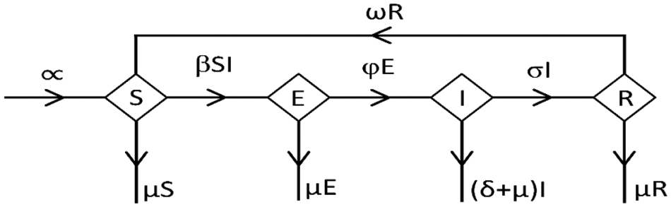
Figure 1: Flowchart of the model
2.1 The Basic Reproductive Number (BRN)
Let
Now
The spectral radius of
The BRN
The system (1) has a disease-free equilibrium (DFE) point
2.3 Stability of Modified SEIR Model
The local stability of the modified SIER model is performed at
3 SEIR Model Modified with Time Delay
This section introduces a time delay parameter τ.
3.1 Delay Differential Equation Model
Incorporating the impact of time delay in infected populations, model (1) assumes the following structure:
The symbol
3.2 The Basic Reproductive Number of Delayed Epidemic Model
Let
Now,
The spectral radius of
The BRN of the delayed epidemic model
The system (3) has a disease-free equilibrium point
3.4 Stability of Modified SEIR Delayed Model
The local stability of the modified SIER model is performed at
4 Numerical Computation of Delayed Epidemic Model
The forward Euler scheme utilized for the model under study method involves making the following supposition can be expressed as follows:
Suppositions:
4.2 Fourth Order Runge Kutta Scheme (RK-4)
Considering the equations of system (3), the study develops an explicit RK-4 method. A numerical scheme for the RK-4 method is constructed as follows:
Step 1
Step 2
Step 3
Step 4
Final Step
4.3 Non-Standard Finite Difference (NSFD) Scheme
The NSFD approach corresponding to (3) is
4.4 Positivity of the NSFD Scheme
Since all state variables within the model represent proportions of a population, it follows that something like one of them should be positive, while the others should remain non-negative consistently. In this context, the theorem presented below provides valuable insight.
Theorem: Assume that
Proof: Now for
Now for
The study assumes that the preceding set of equations guarantees that the values of
Obviously,
4.5 Boundedness of NSFD Scheme
Given that the model is about the human population, it is critical to ensure that at any given time ‘t’, the sum of populations in all compartments does not exceed the overall population. The following theorem addresses this condition effectively:
Theorem: Let
Proof: For bondedness of the proposed NSFD scheme from above, the following can be obtained:
Now for
Since
Consequently
4.6 Convergence Analysis of NSFD Scheme
Let
The Jacobian matrix of the system (35) at the DFE point is given below:
For the above Jacobian matrix, it has eigenvalues
4.7 Consistency of NSFD Scheme
Beginning with the first equation in the system (29), then
The Taylor’s series expansion of the
The following can be obtained from Eq. (36):
After some simplification and applying
From the second equation of the NSFD scheme, it can have
The Taylor’s series expansion of the
Substituting the value of
Apply
From the third equation of the NSFD scheme, the following can be obtained:
The Taylor’s series expansion of the
By applying
From the fourth equation of the NSFD scheme, it can have
The Taylor’s series expansion of the
Similarly,
by substituting (42) in (43) and simplifying it. Hence, the proposed NSFD scheme with the delay effect is consistent with the first order.
By demonstrating global stability, the study provides strong theoretical support for using time-delayed models to understand and manage typhoid fever outbreaks.
Case 1: Trivial Case
Consider a candidate Lyapunov function as follows:
Case 2: Disease-Free Equilibrium
Consider Volterra type Lyapunov function it can have
Case 3: Endemic Equilibrium
From the first equations of system (3)
From the second equation of system (3)
From the third equation of system (3)
From the forth equation of system (3)
Now, it can have
Hence, set
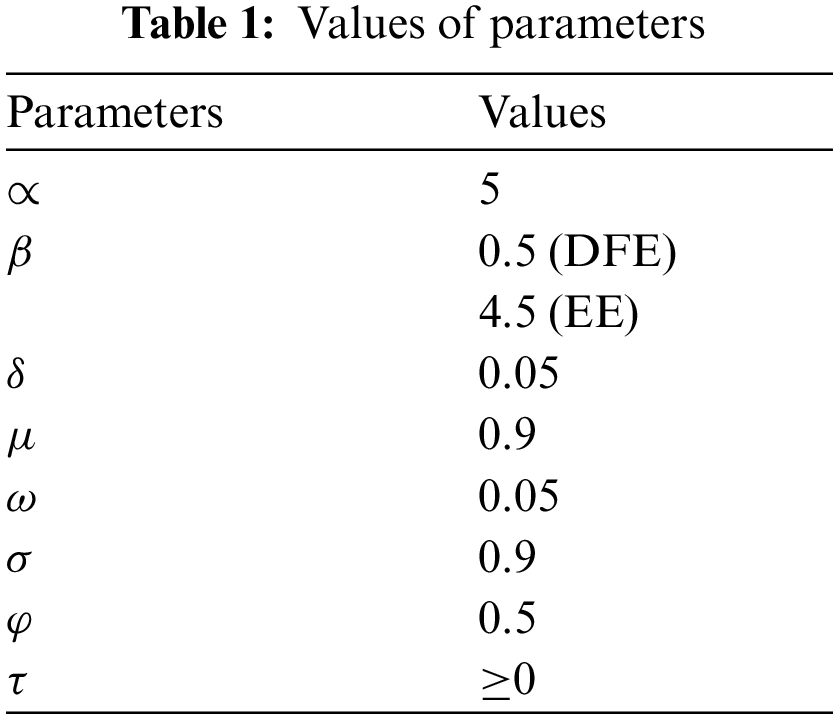
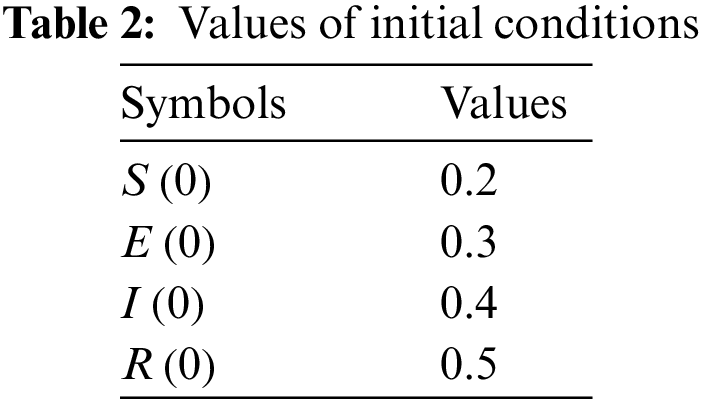
Table 1 lists the parameters employed in numerical simulations, while Table 2 details the initial conditions. The figures illustrate the dynamics of a delayed SEIR model.
In Fig. 2, the forward Euler technique point with a small step size
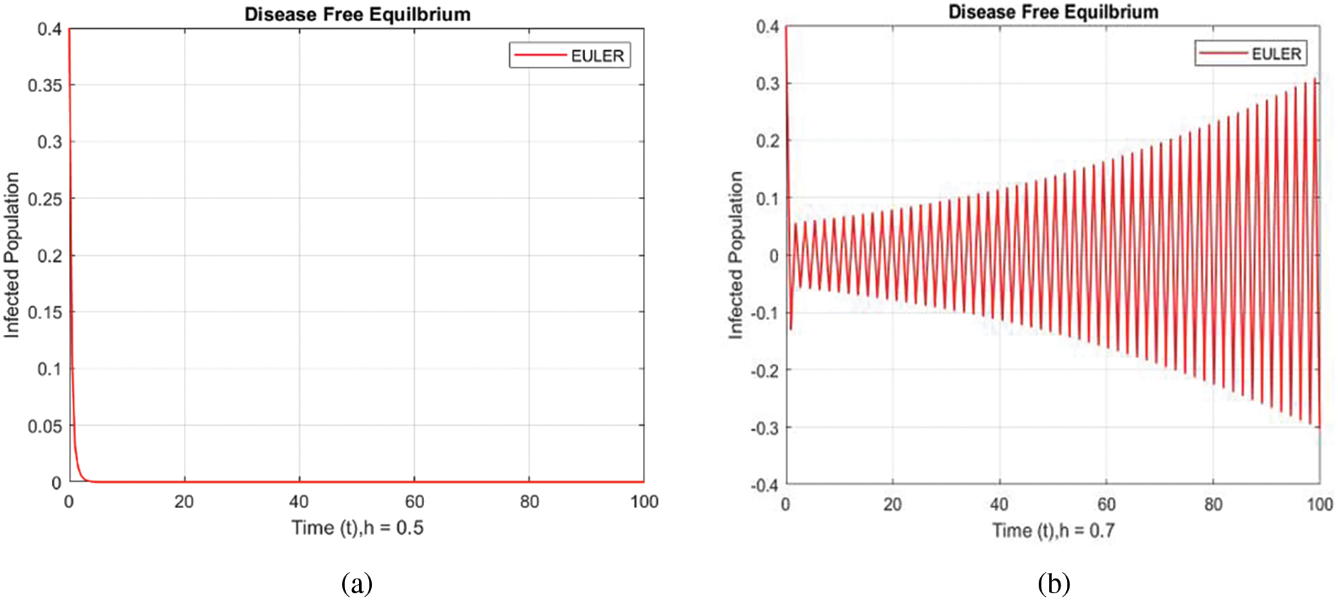
Figure 2: Infected populations at various step sizes employing the Euler approach. (a) h = 0.5, (b) h = 0.7
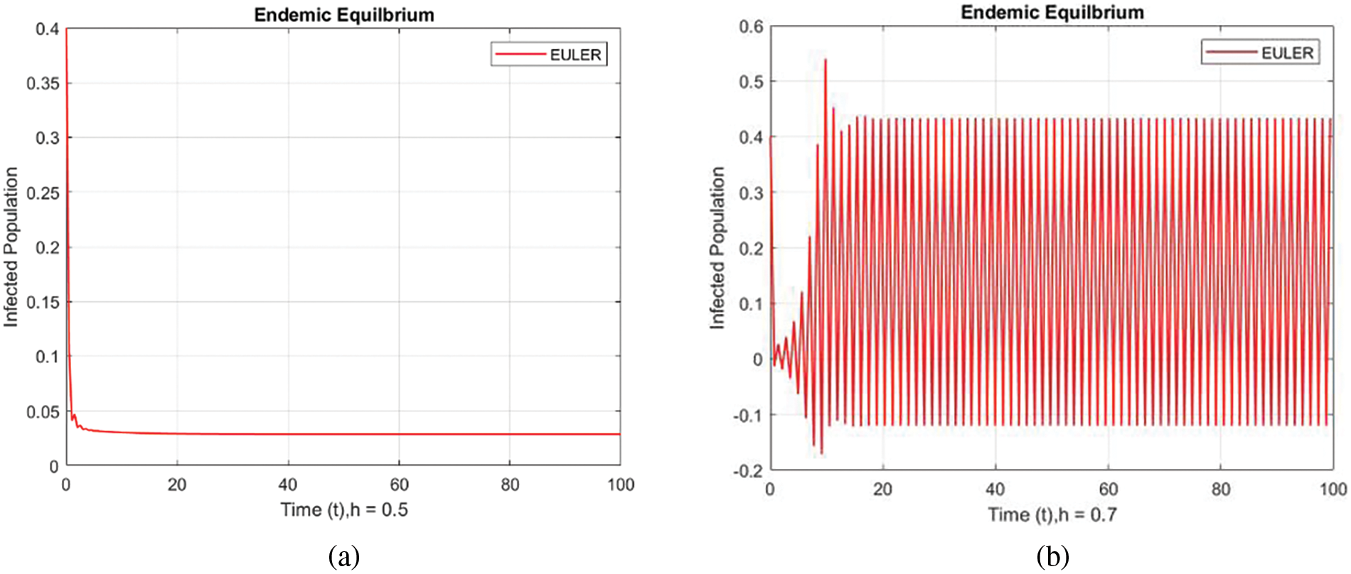
Figure 3: Infected populations at various step sizes employing the Euler approach. (a) h = 0.5, (b) h = 0.7
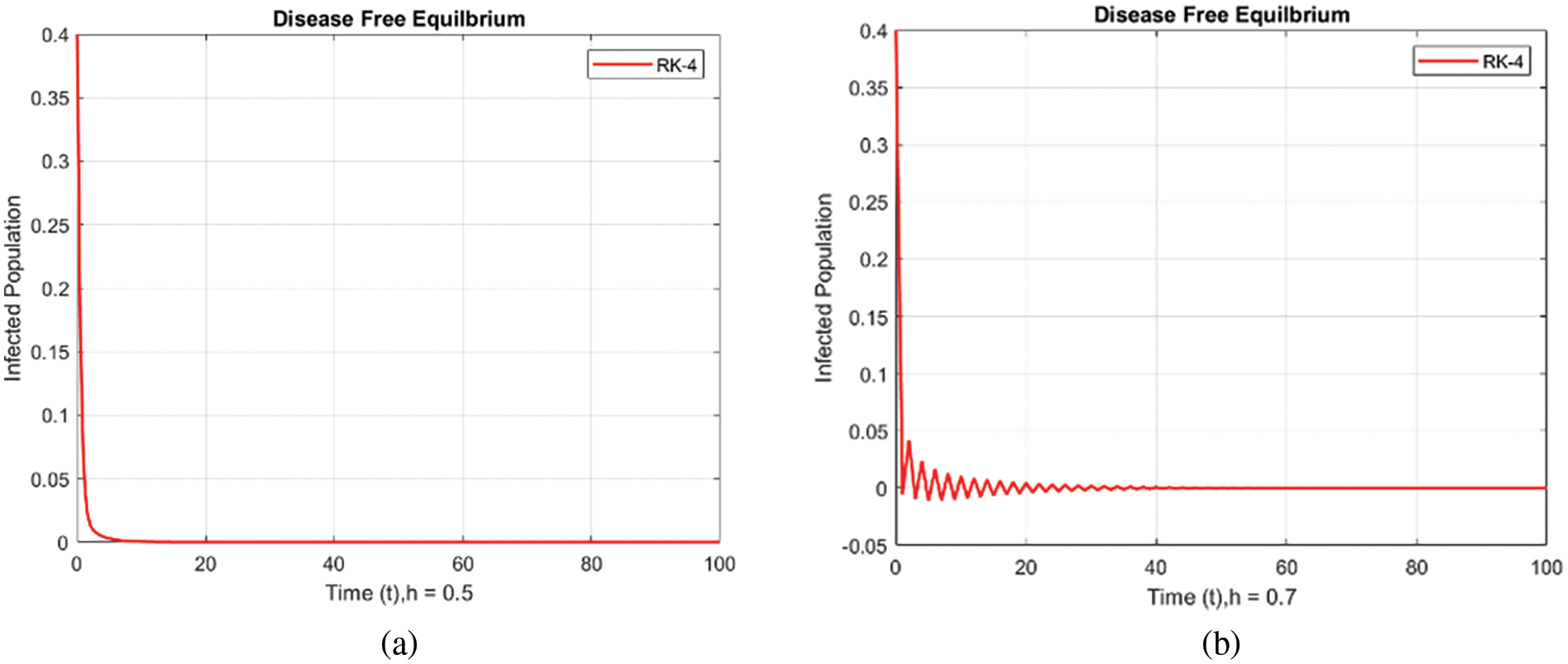
Figure 4: Infected populations at various step sizes employing the RK-4 approach. (a) h = 0.5, (b) h = 0.7
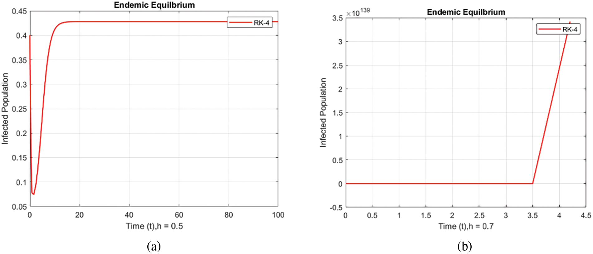
Figure 5: Infected populations at various step sizes employing the RK-4 approach. (a) h = 0.5, (b) h = 0.7
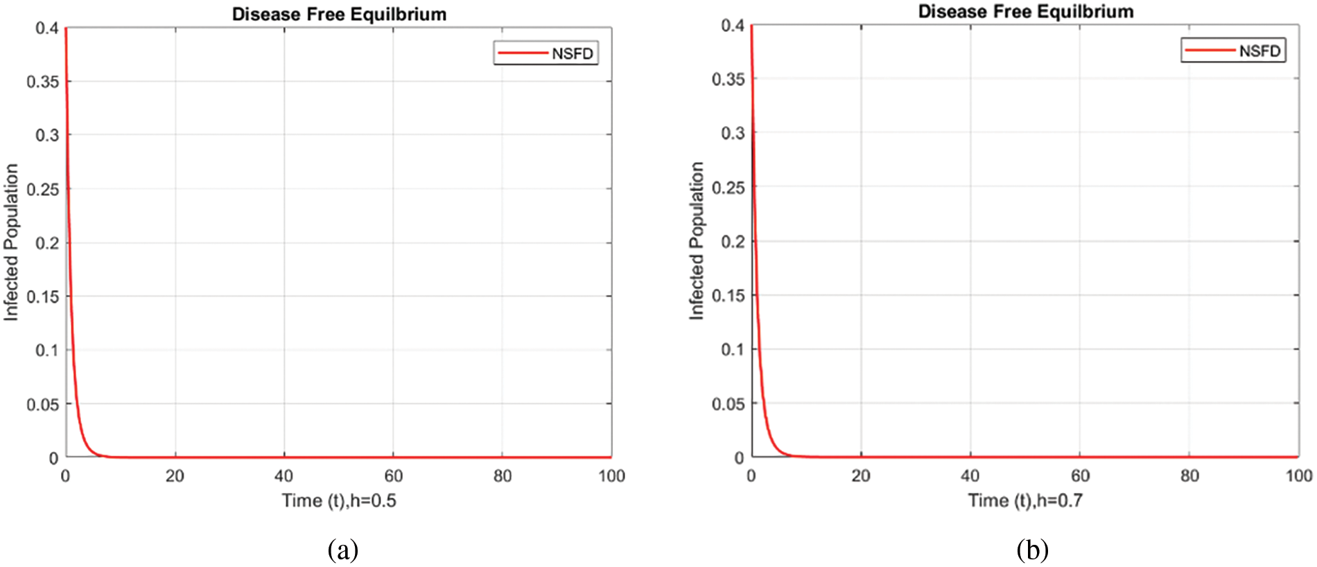
Figure 6: Infected populations at various step sizes employing the NSFD approach. (a) h = 0.5, (b) h = 0.7
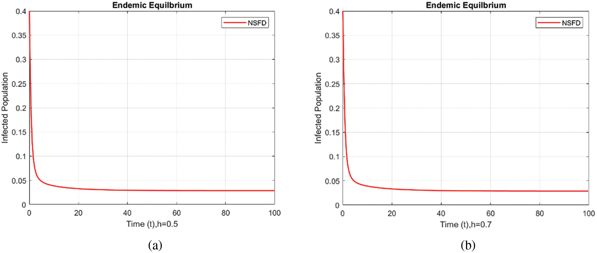
Figure 7: Infected populations at various step sizes employing the NSFD approach. (a) h = 0.5, (b) h = 0.7
Figs. 8 and 9 compare the infected population of a model with and without a time delay factor. The Euler Method demonstrates that introducing a delay can control the endemic status. On the other hand, Figs. 10 and 11 show the behavior of the infected population using the RK-4 approach, resulting in a delay in people getting infected after adding a delay factor in the exposed compartment. In addition, Figs. 12 and 13 indicate that the NSFD scheme is more convergent in a delayed model than without a delay. Fig. 14 outlines charts of infected populations for different values of
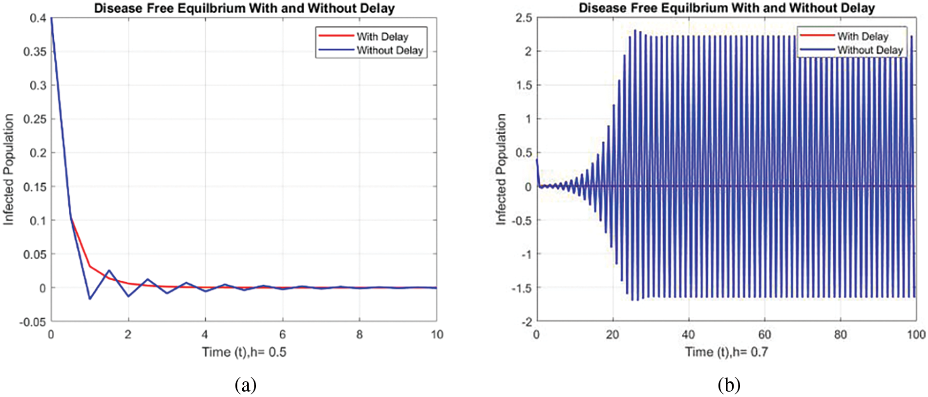
Figure 8: Comparison of the infected population at various step sizes employing the Euler approach. (a) h = 0.5, (b) h = 0.7
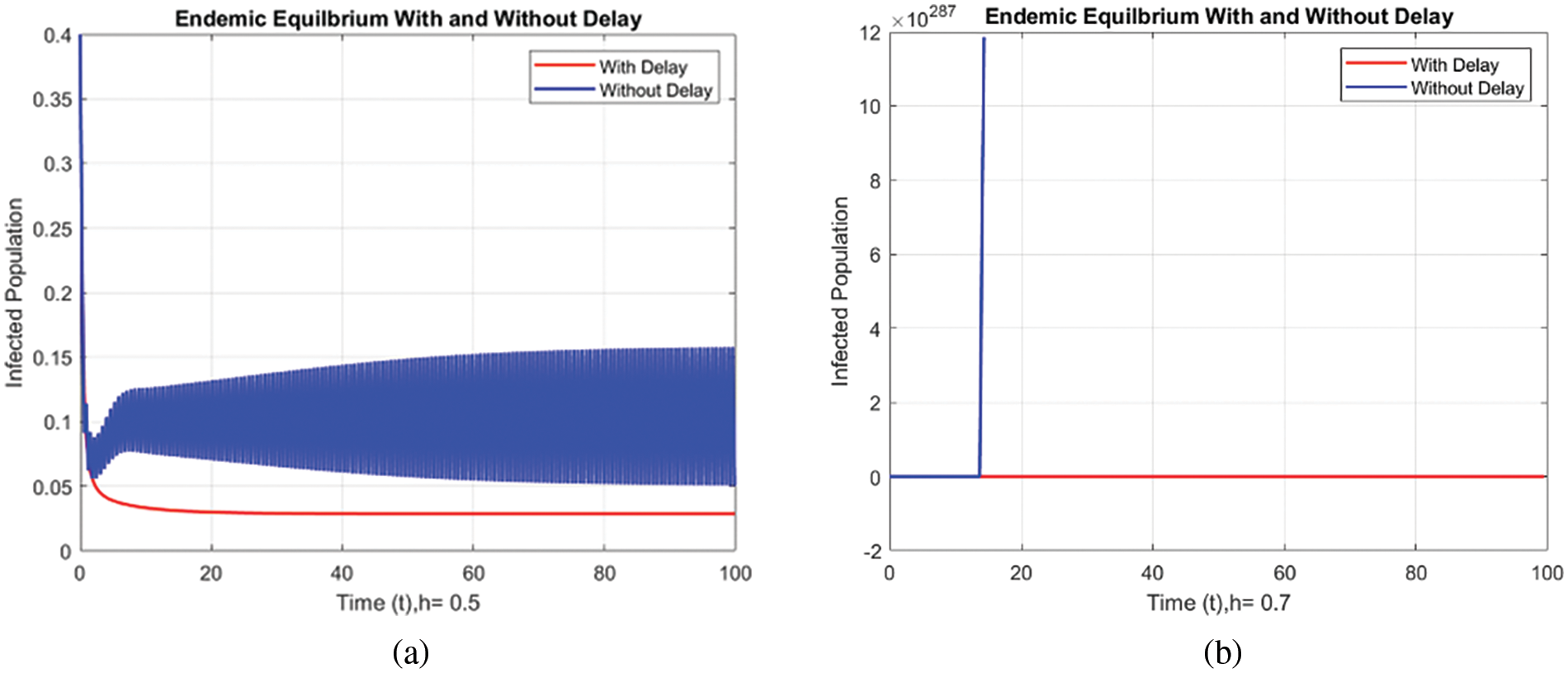
Figure 9: Comparison of the infected population at various step sizes employing the Euler approach. (a) h = 0.5, (b) h = 0.7
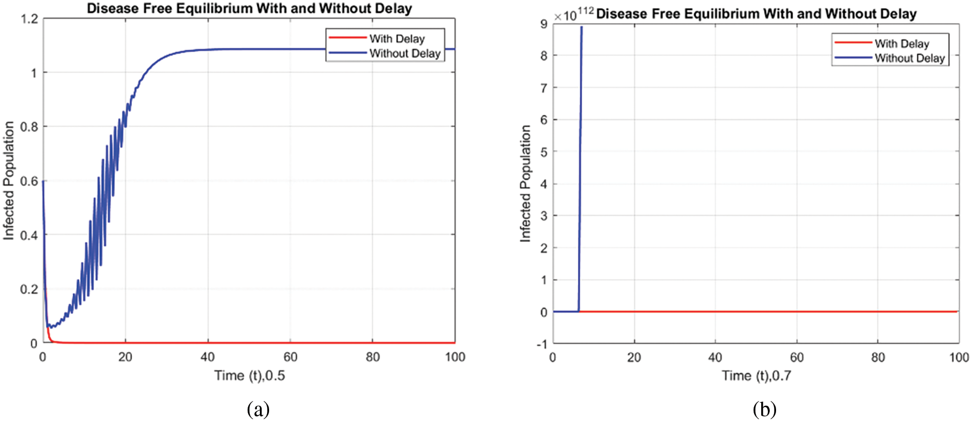
Figure 10: Comparison of the infected population at various step sizes employing the RK-4 approach. (a) h = 0.5, (b) h = 0.7
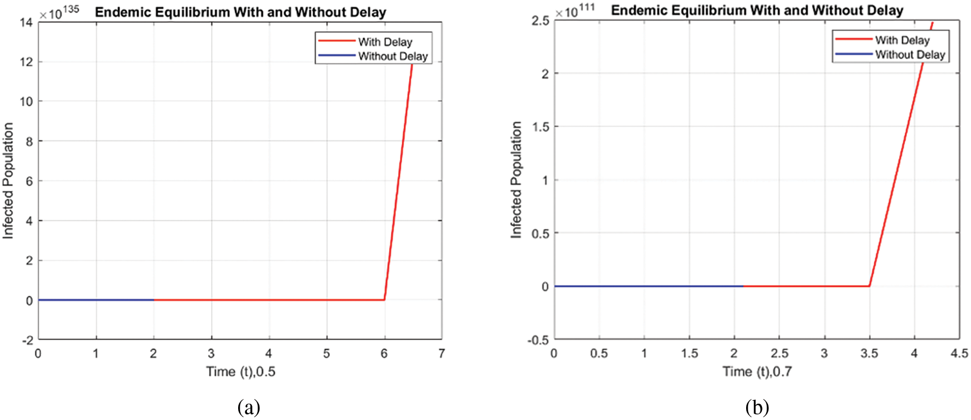
Figure 11: Comparison of the infected population at various step sizes employing the RK-4 approach. (a) h = 0.5, (b) h = 0.7
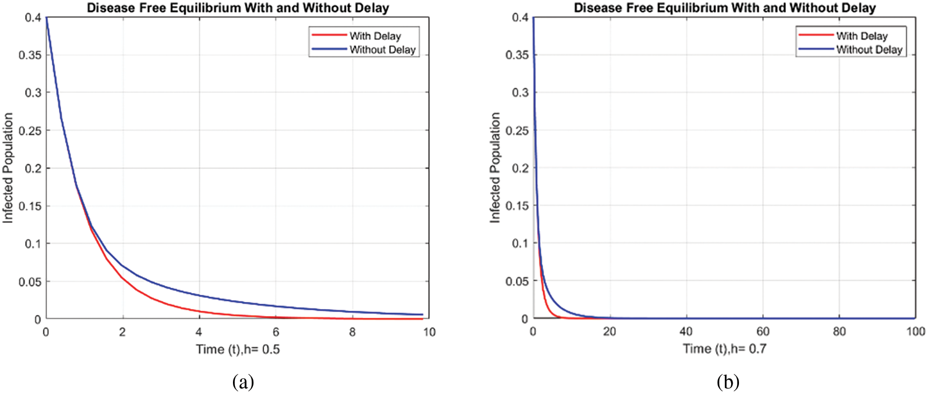
Figure 12: Comparison of Infected population at various step sizes employing NSFD approach. (a) h = 0.5, (b) h = 0.7
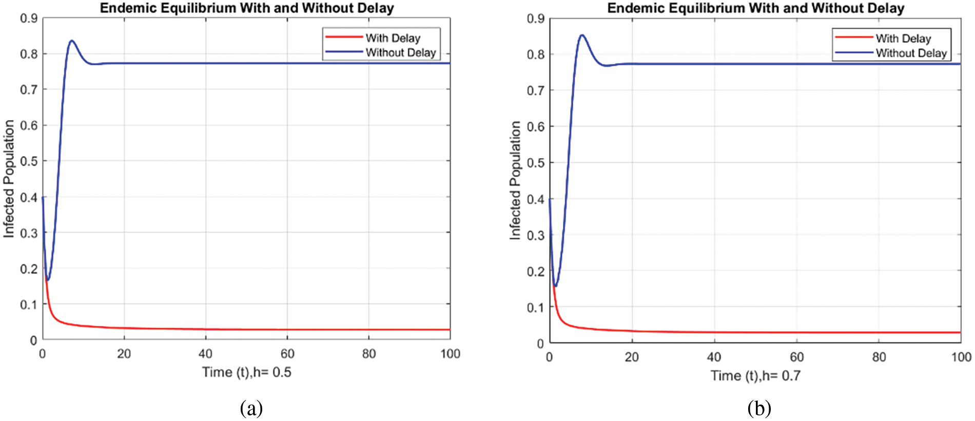
Figure 13: Comparison of the infected population at various step sizes employing NSFD approach. (a) h = 0.5, (b) h = 0.7
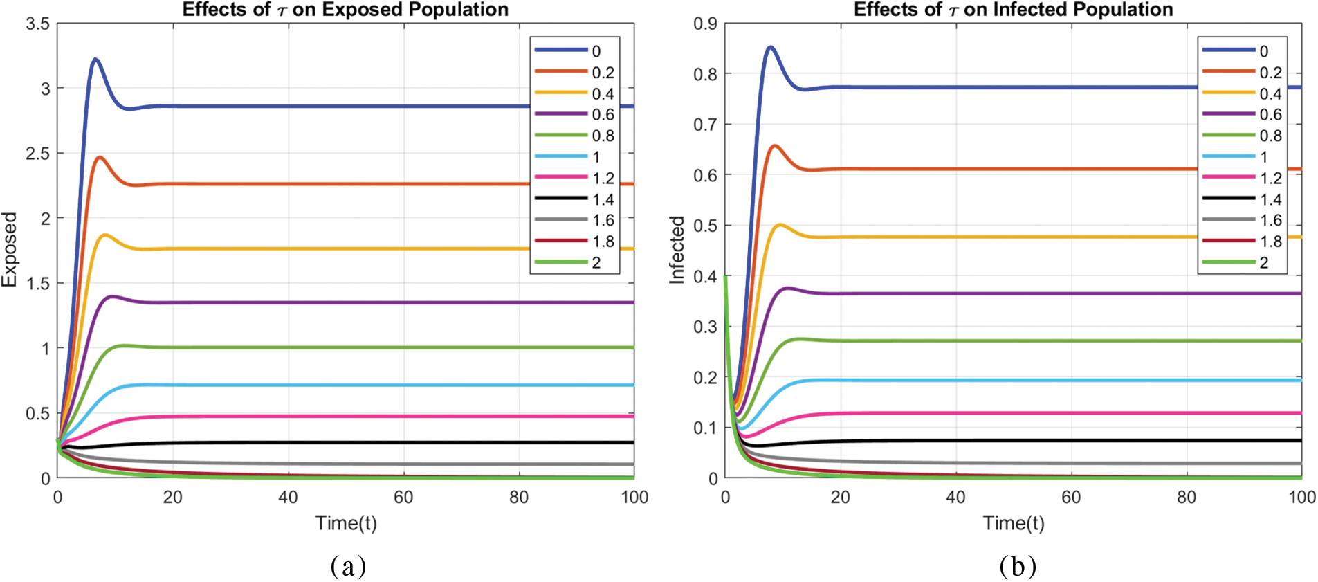
Figure 14: Effect of different values of
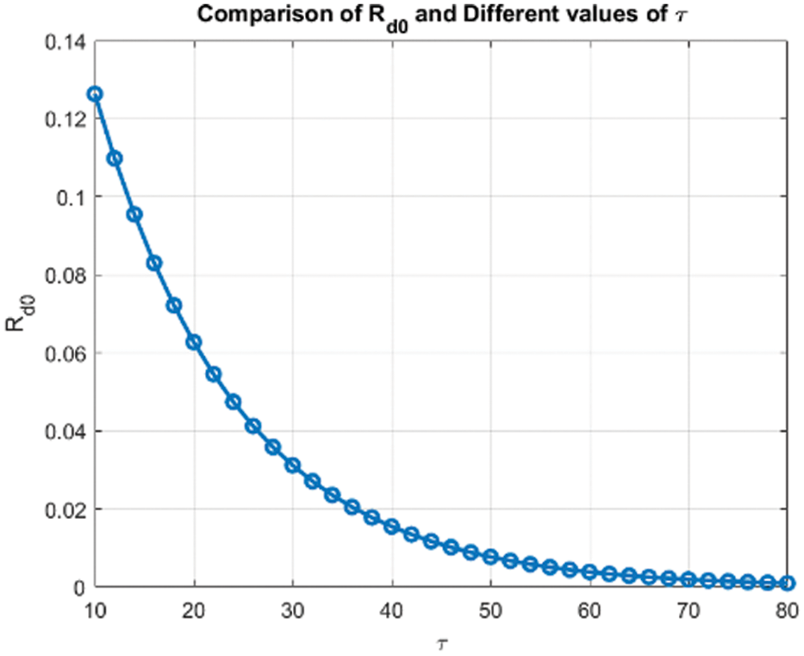
Figure 15: Comparison of
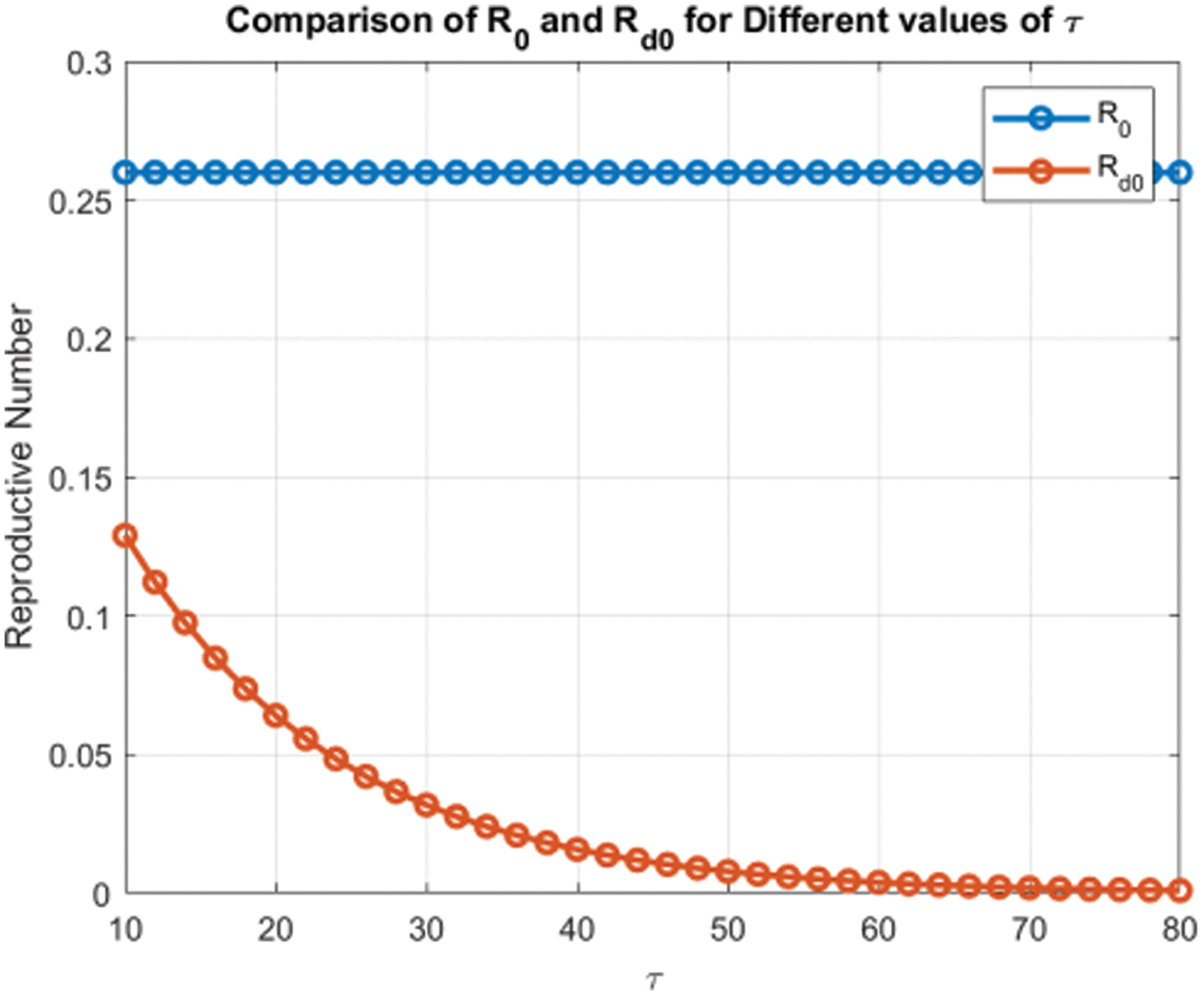
Figure 16: Comparison of
6 Parameter Estimation Analysis
A helpful way to validate the Typhoid delayed epidemic model is by fitting the model parameters to data obtained on the actual typhoid epidemics. All the data for Typhoid fever is collected and compiled from the Integrated Disease Surveillance & Response (IDSR) Report, Center of Disease Control, National Institute of Health, Islamabad. The data consists of the cases reported all over the country for 2023 [42]. It enhances the model, hence a better appreciation of the disease pattern and a better prediction of the future status of the disease. The least squares method of curve fitting is employed to estimate the model’s parameters. Now, it is possible to fit the model’s parameters using the least squares approach using actual data regarding the newly infected typhoid cases in 2023, as indicated in Table 3. Among them, this study selected two parameters, incidence rate φ, and time delay τ, and the remaining parameters provide better estimation based on the actual cases of typhoid fever in Pakistan. It was evident from the fitted model of the number of infected cases per month that the model was accurate in the sense that it predicted the number of infected cases each month. In Fig. 17, the red-filled circles represent the observed values explained in the previous section, while the continuous blue line shows the model’s nonlinear least square curve fitting. This graph appears to indicate that the model in question works quite well in terms of how it addresses the numerical progression of the epidemics of typhoid fever in reality. When it was pointed out that the least squares method was used and the data was real, this ensures that the Typhoid delayed epidemic model indeed simulates the epidemic. In addition, the model can offer information regarding what can prevent the emergence of similar diseases in society in the future.
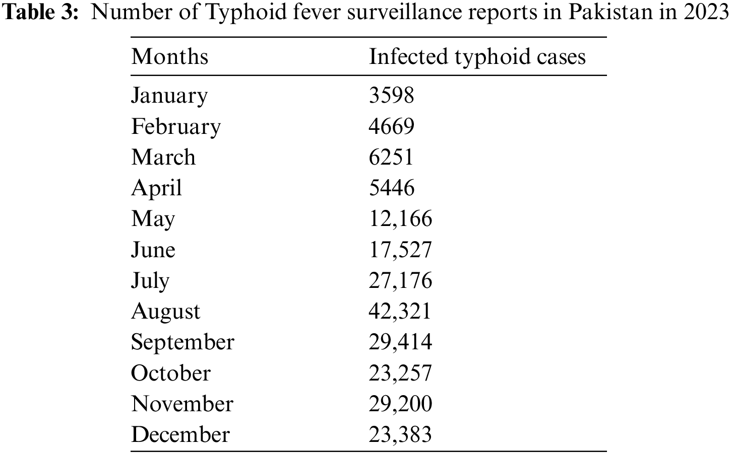
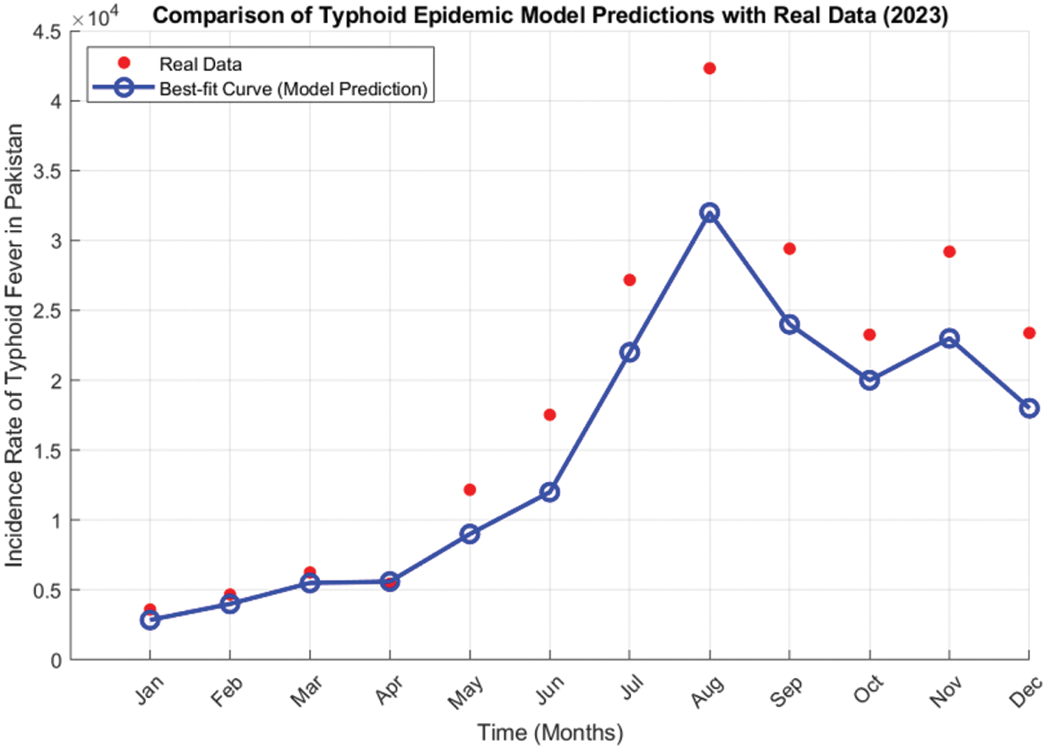
Figure 17: The monthly Typhoid fever cases time series in Pakistan for 2023 and the proposed model’s best-fitted curve
The transmission of typhoid fever caused by Salmonella typhi is examined using a mathematical model that emphasizes the importance of delay in its effectiveness. Time delays can influence the nature of patterns and slow the emergence of patterns in the density of the infected population. The analyzed model is further expanded with equilibrium analysis, reproduction number calculation, and stability analysis. Three numerical techniques, forward Euler, RK-4, and NSFD, are employed to solve the proposed model. Some essential characteristics such as convergence, positivity, boundedness, and consistency are studied, and the developed scheme preserves all these essential features. The calculated results demonstrated the usefulness of the NSFD method in accurately capturing and preserving the essential characteristics of the continuous delayed model. It demonstrated that the proposed NSFD scheme maintains the integrity of the continuous delayed model’s characteristics, positivity, boundedness, and asymptotic stability over all finite step sizes. As a result, it produces dependable approximations, whereas several traditional techniques fail to maintain the critical mathematical properties of the continuous model. As a result, these strategies create solutions that are not just unstable but also negative. Finally, numerical simulations were run to validate the results of the analytical research. This study intends to explore the development of higher-order NSFD schemes tailored for typhoid transmission models. Future directions could include stochastic, fractional, and fuzzy extensions, among other possibilities.
Limitation of study: In the present work, the previous mathematical model of the transmission of Typhoid fever is vindicated using time delay and the NSFD scheme. Some of the limitations include the following: This is a model that is built on some assumptions, and therefore, when obtaining such data in real life, it is essential to check the credibility of the mentioned benchmarks. Still, it is as accurate as the epidemiological data with which the model was supplied, which might be limited or of uneven quality. The utilization of the NSFD scheme can be complex, especially in assigning it, and perhaps more complicated for those with little quantitative proficiency or in places with few resources since the modulated method entails some calculation. NSFD is superior to makeshift solutions, yet there is a specific aspect to consider when choosing a step size. Also, the model does not incorporate geographical factors and other aspects of the environment, which may be disadvantageous in a specific scenario. In order to address these limitations in subsequent studies, it is essential to continuously improve and validate the model to further enhance its usefulness in finding the right strategy for eradicating this health complication.
Acknowledgement: The authors Thabet Abdeljawad and Aiman Mukheimer would like to thank Prince Sultan University for paying the APC and for the support through TAS research lab.
Funding Statement: This work is supported by Prince Sultan University through TAS research lab.
Author Contributions: Conceptualization, methodology, software, and draft manuscript preparation: Muhammad Tashfeen and Fazal Dayan, Formal analysis, methodology, software, validation, and supervision: Muhammad Aziz ur Rehman, Thabet Abdeljawad and Aiman Mukheimer. All authors reviewed the results and approved the final version of the manuscript.
Availability of Data and Materials: The datasets used and/or analyzed during the current study are available from the corresponding author upon reasonable request.
Ethics Approval: Not applicable.
Conflicts of Interest: The authors declare that they have no conflicts of interest to report regarding the present study.
References
1. Masasila NH, Ngeleja RC. Mathematical analysis of the role of information on the dynamics of typhoid fever; 2023. Available from: https://arxiv.org/abs/2310.09825. [Assessed 2024]. [Google Scholar]
2. Ivanoff B, Levine MM, Lambert P. Vaccination against typhoid fever: present status. Bull World Health Organ. 1994;72(6):957. [Google Scholar] [PubMed]
3. Nsutebu EF, Martins P, Adiogo D. Prevalence of typhoid fever in febrile patients with symptoms clinically compatible with typhoid fever in Cameroon. Trop Med Int Health. 2003;8(6):575–8. doi:10.1046/j.1365-3156.2003.01012.x. [Google Scholar] [PubMed] [CrossRef]
4. Shaikh AS, Nisar KS. Transmission dynamics of fractional-order typhoid fever model using Caputo-Fabrizio operator. Chaos Solit Fractals. 2019;128:355–65. doi:10.1016/j.chaos.2019.08.012. [Google Scholar] [CrossRef]
5. Mushayabasa S. Modeling the impact of optimal screening on typhoid dynamics. Int J Dyn Control. 2016;4:330–8. doi:10.1007/s40435-014-0123-4. [Google Scholar] [CrossRef]
6. Adegbola EY. Mathematical modeling of the transmission dynamics of typhoid fever and its control (Ph.D. Thesis). Federal University of Technology: Minna, Nigeria; 2023. [Google Scholar]
7. Suhuyini AK, Seidu B. A mathematical model on the transmission dynamics of typhoid fever with treatment and booster vaccination. Front Appl Math Stat. 2023;9:1151270. doi:10.3389/fams.2023.1151270. [Google Scholar] [CrossRef]
8. Mushayabasa S, Bhunu CP, Ngarakana-Gwasira ET. Mathematical analysis of a typhoid model with carriers, direct and indirect disease transmission. Int J Math Sci Eng Appl. 2013;7(1):79–90. [Google Scholar]
9. Antillón M, Warren JL, Crawford FW, Weinberger DM, Kürüm E, Pak GD, et al. The burden of typhoid fever in low-and middle-income countries: a meta-regression approach. PLoS Negl Trop Dis. 2017;11(2):e0005376. [Google Scholar]
10. Punchihewage-Don AJ, Hawkins J, Adnan AM, Hashem F, Parveen S. The outbreaks and prevalence of antimicrobial resistant Salmonella in poultry in the United States: an overview. Heliyon. 2022;8(11):e11613. [Google Scholar]
11. Mushayabasa S. A simple epidemiological model for Typhoid with saturated incidence rate and treatment effect. Int J Math Comput Sci. 2013;6(6):688–95. [Google Scholar]
12. Nyerere N, Mpeshe SC, Edward S. Modeling the impact of screening and treatment on the dynamics of typhoid fever. World J Model Simul. 2018;14(4):298–306. [Google Scholar]
13. Karunditu JW, Kimathi G, Osman S. Mathematical modeling of typhoid fever disease incorporating unprotected humans in the spread dynamics. J Adv Math Comput Sci. 2019;32(3):1–11. doi:10.9734/jamcs/2019/v32i330144. [Google Scholar] [CrossRef]
14. Mutua JM, Wang FB, Vaidya NK. Modeling malaria and typhoid fever co-infection dynamics. Math Biosci. 2015;264:128–44. doi:10.1016/j.mbs.2015.03.014. [Google Scholar] [PubMed] [CrossRef]
15. Tilahun GT, Makinde OD, Malonza D. Co-dynamics of pneumonia and typhoid fever diseases with cost-effective optimal control analysis. Appl Math Comput. 2018;316:438–59. doi:10.1016/j.amc.2017.07.063. [Google Scholar] [CrossRef]
16. Mushanyu J, Nyabadza F, Muchatibaya G, Mafuta P, Nhawu G. Assessing the potential impact of limited public health resources on the spread and control of Typhoid. J Math Biol. 2018;77:647–70. doi:10.1007/s00285-018-1219-9. [Google Scholar] [PubMed] [CrossRef]
17. Alharbi MH, Alalhareth FK, Ibrahim MA. Analyzing the dynamics of a periodic typhoid fever transmission model with imperfect vaccination. Mathematics. 2023;11(15):3298. doi:10.3390/math11153298. [Google Scholar] [CrossRef]
18. Edward S. A deterministic mathematical model for direct and indirect transmission dynamics of typhoid fever. Open Access Libr J. 2017;4(5):1–16. [Google Scholar]
19. Musa SS, Zhao S, Hussaini N, Usaini S, He D. Dynamics analysis of typhoid fever with public health education programs and final epidemic size relation. Results Appl Math. 2021;10:100153. [Google Scholar]
20. Peter OJ, Ibrahim MO, Edogbanya HO, Oguntolu FA, Oshinubi K, Ibrahim AA, et al. Direct and indirect transmission of typhoid fever model with optimal control. Results Phys. 2021;27:104463. [Google Scholar]
21. Edward S, Nyerere N. Modelling typhoid fever with education, vaccination and treatment. Eng Math. 2016;1(1):44–52. [Google Scholar]
22. Nwokoye CH, Umeh II. The SEIQR-V model: on a more accurate analytical characterization of malicious threat defense. Int J Inf Technol Comput Sci. 2017;9(12):28–37. [Google Scholar]
23. Wang C, Chai S. Hopf bifurcation of an SEIRS epidemic model with delays and vertical transmission in the network. Adv Differ Equ. 2016;2016(1):1–19. doi:10.1186/s13662-016-0793-7. [Google Scholar] [CrossRef]
24. Bailey NT. The mathematical theory of infectious diseases and its applications. London: Charles Griffin & Company Ltd.; 1975. [Google Scholar]
25. Suleman M, Riaz S. Unconditionally stable numerical scheme to study the dynamics of hepatitis B disease. Punjab Univ J Math. 2017;49(3):99–118. [Google Scholar]
26. World Health Organization. Typhoid vaccines: WHO position paper, March 2018–recommendations. Vaccine. 2019;37(2):214–6. [Google Scholar]
27. Sulaiman W. Typhoid and malaria co-infection-an interesting finding in the investigation of a tropical fever. Malays J Med Sci. 2006;13(2):64. [Google Scholar] [PubMed]
28. Saade M, Ghosh S, Banerjee M, Volpert V. Delay epidemic models determined by latency, infection, and immunity duration. Math Biosci. 2024;370:109155. doi:10.1016/j.mbs.2024.109155. [Google Scholar] [PubMed] [CrossRef]
29. Jiang J, Zhou T. The influence of time delay on epidemic spreading under limited resources. Physica A. 2018;508:414–23. doi:10.1016/j.physa.2018.05.114. [Google Scholar] [CrossRef]
30. Guglielmi N, Iacomini E, Viguerie A. Delay differential equations for the spatially resolved simulation of epidemics with specific application to COVID-19. Math Methods Appl Sci. 2022;45(8):4752–71. doi:10.1002/mma.8068. [Google Scholar] [PubMed] [CrossRef]
31. Yau MA. Analysis of spatial dynamics and time delays in epidemic models (Ph.D. Thesis). University of Sussex: Brighton, UK; 2014. [Google Scholar]
32. Das K, Chinnathambi R, Srinivas MN, Rihan FA. An analysis of time-delay epidemic model for TB, HIV, and AIDS co-infections. Results Control Optim. 2023;12:100263. doi:10.1016/j.rico.2023.100263. [Google Scholar] [CrossRef]
33. Goel K, Nilam. A mathematical and numerical study of a SIR epidemic model with time delay, nonlinear incidence and treatment rates. Theory Biosci. 2019;138(2):203–13. doi:10.1007/s12064-019-00275-5. [Google Scholar] [PubMed] [CrossRef]
34. Ghosh S, Volpert V, Banerjee M. An epidemic model with time delay determined by the disease duration. Mathematics. 2022;10(15):2561. doi:10.3390/math10152561. [Google Scholar] [CrossRef]
35. Shoaib Arif M, Raza A, Abodayeh K, Rafiq M, Bibi M, Nazeer A. A numerical efficient technique for the solution of susceptible infected recovered epidemic model. Comput Model Eng Sci. 2020;124(2):477–91. doi:10.32604/cmes.2020.011121. [Google Scholar] [CrossRef]
36. Abodayeh K, Raza A, Arif MS, Rafiq M, Bibi M, Mohsin M. Stochastic numerical analysis for impact of heavy alcohol consumption on transmission dynamics of gonorrhoea epidemic. Comput Mater Contin. 2020;62(3):1125–42. doi:10.32604/cmc.2020.08885. [Google Scholar] [CrossRef]
37. Shatanawi W, Raza A, Arif MS, Rafiq M, Abodayeh K, Bibi M. An effective numerical method for the solution of a stochastic coronavirus (2019-nCoV) pandemic model. Comput Mater Contin. 2021;66(2):1121–37. doi:10.32604/cmc.2020.012070. [Google Scholar] [CrossRef]
38. Saleem S, Rafiq M, Ahmed N, Arif MS, Raza A, Iqbal Z, et al. Fractional epidemic model of coronavirus disease with vaccination and crowding effects. Sci Rep. 2024;14(1):8157. doi:10.1038/s41598-024-58192-7. [Google Scholar] [PubMed] [CrossRef]
39. Raza A, Baleanu D, Khan ZU, Mohsin M, Ahmed N, Rafiq M, et al. Stochastic analysis for the dynamics of a poliovirus epidemic model. Comput Model Eng Sci. 2023;136(1):257–75. doi:10.32604/cmes.2023.023231. [Google Scholar] [CrossRef]
40. Cheng X, Wang Y, Huang G. Global dynamics of a network-based SIQS epidemic model with nonmonotone incidence rate. Chaos Solitons Fractals. 2021;153:111502. doi:10.1016/j.chaos.2021.111502. [Google Scholar] [PubMed] [CrossRef]
41. Khan IU, Mustafa S, Shokri A, Li S, Akgül A, Bariq A. The stability analysis of a nonlinear mathematical model for typhoid fever disease. Sci Rep. 2023;13(1):15284. doi:10.1038/s41598-023-42244-5. [Google Scholar] [PubMed] [CrossRef]
42. Integrated Disease Surveillance & Response (IDSR) Report. Center of Disease Control, National Institute of Health, Islamabad; 2024. Available from: https://nih.org.pk/idsr-weekly-bulletin. [Accessed 2024]. [Google Scholar]
Cite This Article
 Copyright © 2024 The Author(s). Published by Tech Science Press.
This work is licensed under a Creative Commons Attribution 4.0 International License , which permits unrestricted use, distribution, and reproduction in any medium, provided the original work is properly cited.
 Downloads
 Citation Tools