A Non-Intrusive Stochastic Phase-Field for Fatigue Fracture in Brittle Materials with Uncertainty in Geometry and Material Properties

Nomenclature

1  Introduction

Material fatigue is a localized and progressive structural damage phenomenon in materials when subjected to repeated cyclic loads far below the monotonic strength of the material [1]. Even though fatigue failures are traditionally associated with metallic materials, this unique failure mode is widespread and is of significant concern for designers and engineers. These failures can result in catastrophic consequences if not adequately understood and managed. Fatigue failure of materials occurs in multiple stages: initiation or formation, micro-crack growth and macro-crack growth. Earlier studies to predict fatigue life were experimental, with little or no usage of predictive and numerical methods [1]. Studies carried out by Wohler [2] to determine the relation between number of cycles to failure (Nf) and applied stress amplitude (σa) were one of the earliest systematic approaches to understand fatigue failure in metals. Fatigue failure of materials can be classified into three different types based on the number of cycles to failure: Oligocyclic (OC), Low cycle (LC) and High Cycle (HC) fatigue.

The earlier approach to fatigue life predictions used various relationships to predict the number of strain and stress cycles the material has to undergo to fail from Wöhler curves. These approaches cannot be applied to model multi-axial fatigue failures and are limited to uniaxial cases of constant amplitude cycles. Paris et al. [3] proposed a relationship between stress intensity factor and crack growth per cycle, widely known as Paris law. Improvements to the above law have resulted in NASGRO (NASA/FLAGRO) equations that reproduce real-life fatigue behaviour like nucleation, crack closure and load effects. All the above approaches require calibration of problem-specific parameters and cannot be generalized for arbitrary materials.

Works on computational modelling of damage to date can be broadly categorized into two types based on their approach—discrete and diffuse/smeared method. Discrete methods model cracks as a discrete quantity. In earlier approaches, crack growth was modelled via node splitting, and each node split created a fresh fracture plane and a new discontinuity for crack propagation. Hence, such models showed high mesh dependency and constrained crack growth along element edges. The automatic re-meshing approach developed by Ingraffea et al. [4] addressed the mesh bias problem to a large extent. Another prominent discrete modelling technique is Cohesive zone model (CZM) proposed by Dugdale [5] and Barenblatt [6]. In CZM, the fracture is a gradual process, and separation occurs between the crack tip’s virtual surfaces. Another discrete modelling approach that has gained prominence in the late 90s is the Extended Finite Element Method (XFEM) [7]. XFEM technique avoids mesh manipulation, resolves stress singularities and enables local enrichment of nodes using the partition of unity method. XFEM has also been extended to model fatigue fracture [8]. However, this approach suffers from increased computational complexity compared to traditional Finite Element Method (FEM). Another school of thought assumes crack to be a continuum. Though the discrete approach satisfies our physical intuition, the smeared approach may be better suited to simulate the cracks. Rashid et al. [9] introduced this approach while working on concrete specimens. Here, the effect of crack formation and propagation on properties like stiffness and stress are incorporated into the constitutive model. An introduction of a crack converts an isotropic specimen into an orthotropic specimen due to loss of stiffness in a direction orthogonal to the crack, also known as the Plane of Degradation (POD). Peridynamics [10] is a non-local approach and is one of the most recent and popular diffuse approaches to crack modelling. In this approach, material points interact with each other over finite distances called horizon size and use integro-differential equations, unlike classical continuum mechanics. This approach has also been extended to model fatigue fracture [11] recently and offers numerous advantages due to its ability to naturally handle discontinuities and complex crack interactions without needing predefined paths or criteria.

In this paper, low-cycle fatigue fracture in brittle materials is modelled using Phase-Field Modelling (PFM) technique in a finite element framework. Even though the PFM approach was developed to model solidification problems [12], this technique has emerged as a transformative approach to model fracture processes such as crack nucleation, growth, merging and branching. PFM is based on a variational framework [13] and recasts the critical energy theory of Griffith’s [14] to an energy minimization problem. Variational problem is regularized [15] for efficient numerical implementation, and a scalar field parameter, ϕ∈[0,1], is introduced to model crack and its growth. PFM approach is widely investigated to model various material properties such as anisotropy [16], hyper-elasticity [17], thermo-poroelasticity [18], visco-elasticity [19], ductility [20], functionally gradation [21], chemo-mechanical coupling [22,23], thermo-mechanical coupling [24], piezo-electricity [25,26]. This technique is also extended to model crack propagation in rocks [27], biological tissues [28], brittle materials [29], concrete [30], polymers [31] and composites [32]. Fracture modes such as dynamic cracking [33,34], thermal fracture [35], hydro-fracture [36] and compressive shear fracture [37] have been modelled using phase-field method.

This modelling technique has been very recently extended for simulating fatigue fracture. Boldrini et al. [38] simulated fatigue fracture by introducing another continuous field variable for fatigue in addition to the PF variable. Although this approach could reproduce fatigue under small strains, it failed to reproduce the S-N curves. The degradation potential introduced by Alessi et al. [39] used accumulated strain to degrade the fracture toughness. This approach could not only model S-N curves but also reproduce mean stress effects and multi-axial loading to a great extent. In the PF models proposed by Mesgarnejad et al. [40], fracture toughness was set as a global material property and degraded in the crack tip region. This approach could capture Paris law with high exponents. Grossman-Ponemon et al. [41] extended the above model and fracture toughness was modelled as a function of spatial coordinates and N. Lo et al. [42] introduced a viscous parameter modelled using power law into standard PFM for capturing fatigue crack growth. Caputo et al. [43] and Amendola et al. [44] used Ginzburg-Landau formalism for fatigue crack problems wherein the degradation is modelled by introducing a fatigue potential. Another approach to PFM of fatigue fracture is to degrade the fracture energy [45] as the crack progresses. Ulloa et al. [46] have extended this approach to elastoplastic materials. An additional energy term was introduced to the standard PF model by Schreiber et al. [47] to model fatigue and irreversibility. This approach could reproduce fatigue growth under varying stress ratios and stress amplitudes. Recently, Hasan et al. [48] introduced a new fatigue degradation function and a fatigue history variable. Crack initiation, propagation and final failure could be modelled using this approach, including load and stress ratio effects. Baktheer et al. [49] used the phase-field cohesive zone modelling (PF-CZM) technique to evaluate fatigue behaviours in quasi-brittle materials like concrete.

The specimen’s material properties, geometric parameters, and loading conditions are treated as deterministic in all the aforementioned studies. Studies are carried out for mean, minimum and maximum value without acknowledging the inherent variability in material properties, geometry and applied loads. For a realistic assessment of system response and to arrive at an optimal design that balances safety, efficiency, and performance for critical applications like aerospace, bio-medical and nuclear, a probabilistic approach is more realistic [50]. A probabilistic approach to design is pertinent for the realistic assessment of safety risks, addressing unforeseen life extension requirements, and responding to the dynamic evolution of design criteria over the operational lifespan of structures.

The most common and straightforward technique to determine the uncertainty in dependent response is to employ Monte Carlo simulation (MCS) approach [51]. The technique mentioned above relies on generating many random inputs, observing their impact on the system, and generating a statistical distribution of all possible outcomes. Even though the method is easy to implement, the number of input samples required to represent the dependent variable response accurately will be typically 105 or more. For complex engineering problems with millions of DOFs, the MCS approach will result in substantial overheads like increased computation time and resources. Another commonly applied probabilistic method is the perturbation technique [52], which uses Taylor series expansion to obtain local approximation of dependent variables. Applying perturbation techniques is frequently limited to first and second-order and higher orders are computationally demanding. This approach finds application for systems with low variability in independent parameters, as in aerospace engineering, where stringent quality control is followed [53]. In the Polynomial Chaos Expansion (PCE) approach [54], a polynomial basis represents the dependent variables of interest. The polynomial is decomposed such that uncertainty is associated with the polynomial part, and the coefficients of the polynomial become deterministic. In earlier days, PCE approaches were intrusive and required extensive modification of the existing deterministic parent codes. Non-intrusive PCE techniques [55] were later introduced as an added improvement. The sensitivity of random independent variables on dependent variables of interest can also be readily determined by computing Sobol’ indices from PCE coefficients [56]. PCE technique is widely applied for uncertainty quantification in various engineering fields [57,58]. In the last decade, numerous stochastic crack growth studies have been carried out [57–59] using various probabilistic approaches. Numerous probabilistic models have been proposed for fatigue over the past few decades [60,61]. Experimental fatigue tests to quantify uncertainty are extremely costly and time-consuming.

In this paper, the authors propose a non-intrusive PCE-based stochastic method to study low-cycle fatigue fracture in brittle materials utilizing the PFM framework to account for uncertainties in material properties and geometric parameters. In PCE approach, the objective is to account an equivalent model without any loss of generality to overcome prohibitively expensive simulations to conduct various iterations. This general equivalent model involves running the simulation to represent the characteristics of the numerical model. Unlike traditional methods that often demand substantial computational resources and intrusive modifications to finite element codes, the proposed framework offers a streamlined solution with little or no computational overheads. Sensitivity analysis is carried out to determine the dominant parameters when multiple random independent variables are present in the system. Leveraging Sobol’ indices for sensitivity analysis provides valuable insights into the influence of random variables on system response. Sensitivity studies can be carried out by post-processing the coefficients of PCE polynomials. This innovative framework not only facilitates precise estimation of the number of cycles to failure but also offers a practical, efficient, and non-intrusive tool for probabilistic studies in sensitive engineering applications, empowering informed decision-making and risk assessment.

The paper is organized as follows: General mathematical formulations for fatigue phase-field are provided in Section 2. Governing equations, finite element discretization and solution schemes are presented in Section 3. Section 4 touches upon the fundamentals of PCE for modelling systems dependent variable response and sensitivity analysis. Applications of the PCE technique to evaluate the low cycle fracture characteristic in a brittle fatigue crack growth problem are demonstrated in Section 5 using multiple two-dimensional numerical problems having random geometric and material variables. Concluding remarks of this manuscript are given in Section 6.

2  Phase-Field Fatigue Fracture Model

This section gives the basics of PFM developed to model rate-independent fatigue fracture under quasi-static conditions. Small strain, irreversibility of any dissipative forces and smooth loading in time are assumed to hold, while inertial effects, wave propagation and thermal effects are neglected in this model. Heat and sound release due to the generation and growth of crack surfaces are also ignored. The governing equations are derived based on energy principles. Consider an arbitrary linear elastic n dimensional body (Ω⊂Rn,n∈{2,3}) undergoing brittle fracture. The surface of the body, Γ⊂Rn−1, is decomposed to Γ=∂Γ1∪∂Γ2. Γ1 and Γ2, represents two disjoint surfaces where t(x) for x∈Γ1 and u0(x) for x∈Γ2 is the traction (Neumann boundary condition) and applied displacement (Dirichlet boundary condition), respectively. Let Γs represent the evolving crack surface. Let b(x) for x∈Ω represent the body forces. The total internal energy potential of the body (Ψint) is sum of surface energy (Ψs) and bulk energy (Ψb):

Ψint=Ψs+Ψb(1)

Fracture energy can be calculated from the critical energy release rate (Gc) and is defined as

Ψs=∫ΓsGcdΓ(2)

Computing Ψs requires explicit tracking of Γs. Tracking Γs for 2D and 3D problems with multiple crack branching and coalescence is computationally expensive and numerically difficult. The sharp crack surface is diffused using a scalar parameter [62] such that the surface integral form of Ψs can be rewritten into a domain integral form. An auxiliary variable called phase-field parameter (ϕ∈[0,1]) is introduced to track crack growth in the domain. A schematic representation of an arbitrary body with sharp and diffused cracks is given in Fig. 1. This scalar parameter is 0 for sound material and 1 for fully damaged material. The domain integral form [63] of Eq. (2) is

Ψs=∫ΓsGcdΓ≈Gc∫ΩI(ϕ,ϕ′)dΩ(3)

where Gc is not dependent on position within the material. I(ϕ,ϕ′) in the above expression is defined as

I(ϕ,ϕ′)=14cw{ℓo(∇ϕ)T⋅(∇ϕ)+w(ϕ)ℓo}(4)

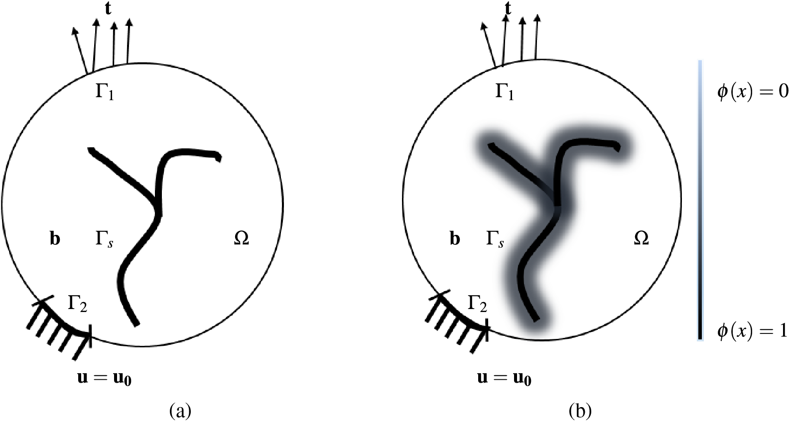
Figure 1: Schematic representation of a solid body with (a) Sharp and (b) Diffused crack

In Eq. (4), ℓo is the length scale parameter (regularization length) and determines the extent of smearing of the crack. The larger the value of ℓo, the more diffused the crack is assumed to be and vice versa. cw and w(ϕ) are the scaling constant and dissipation function, respectively. Choice of w(ϕ) cannot be arbitrary and is expected to fulfil certain conditions [64]:

w(0)=0;w(1)=1;w′(ϕ)≥0forϕ∈[0,1](5)

Based on the choice of w(ϕ) and cw, the phase-field models are widely classified as AT1 (Ambrosio-Tortorelli) [65] and AT2 models [66]. The functional forms for w(ϕ) and cw employed in the AT1 and AT2 models are given below:

AT1 model:

w(ϕ)=ϕandcw=23(6a)

AT2 model:

w(ϕ)=ϕ2andcw=12(6b)

From Eq. (6b), it can be observed that AT2 is a second-order phase-field model. Since w′(ϕ)=0 has a vanishing threshold once the crack initiates, this leads to a material model without a linear elastic branch. This model has been widely used to simulate various fracture phenomena, including crack branching, interaction between multiple cracks, and fracture in heterogeneous materials. The technique is widely validated against experimental data and benchmark problems. On the other hand, the AT1 model (Eq. (6a)) uses first-order PFM and has an initial linear elastic constitutive behaviour. Numerical simulations in this work use AT2 model. Substituting Eqs. (6b) and (4) in Eq. (3) leads to

Ψs=Gc2∫Ω(ϕ2ℓo+ℓo|∇ϕ|2)dΩ(7)

The bulk energy term in Eq. (1) can be written as

Ψb(ϕ,ϵ)=∫Ωg(ϕ)Ψe(ϵ)dΩ(8)

In the above equation, Ψe is the elastic strain energy, and g(ϕ) is the crack degradation function employed to model the reduction in material stiffness due to crack growth. The degradation function should satisfy [63]:

g(0)=1;g(1)=0;g′(ϕ)≤0forϕ∈[0,1](9)

Although degradation functions are available in various forms satisfying Eq. (9), the function chosen for this paper is given below [62]:

g(ϕ)={(1−ϕ)2+k}(10)

where k≈10−6 is the stress degradation constant that prevents numerical singularities during computation. Elastic strain energy for a material at any point is defined as:

Ψe=12ϵ:C:ϵ(11)

In Eq. (11), C and ϵ=∇s(u) are the fourth-order elasticity and small strain tensor, respectively and u is the unknown displacement field variables and ∇s is the symmetric gradient operator. Ψint is redefined by substituting the expressions given in Eqs. (8) and (7) in Eq. (1):

Ψint=∫Ω{g(ϕ)Ψe(ϵ)+Gc2(ϕ2ℓo+ℓo|∇ϕ|2)}dΩ(12)

External work increment δWext is defined as

δWext=δΨext=∫Ωb⋅δu dΩ +∫Γ1t⋅δu dΓ (13)

Internal work increment δWint is defined as

δWint=δΨint=∂Ψint∂ϵδϵ+∂Ψint∂ϕδϕ=∫Ωs⋅δϵ dΩ+∫Ω−2(1−ϕ)δϕΨe(ϵ) dΩ+∫ΩGc(ℓo∇ϕ⋅∇δϕ+1ℓoϕδϕ) dΩ (14)

In the above expression, s is the degraded cauchy stress tensor and is given by

s=g(ϕ)∂Ψe(ϵ)∂ϵ(15)

δWint−δWext=0 should hold true for any random values of δu and δϕ. Applying the divergence theorem to Eq. (14) gives the following governing equations:

∇⋅s+b=0 in Ω(16a)

−Gcℓo∇2ϕ+{Gcℓo+2Ψe(ϵ)}ϕ=2Ψe(ϵ) in Ω(16b)

s⋅n^=t  on  Γ1(16c)

u=u0  on  Γ2(16d)

∇ϕ⋅n^=0 in Γ(16e)

Eqs. (16a) and (16b) are coupled stress and phase-field equilibrium equations, respectively. Eqs. (16c) and (16d) gives the natural and essential boundary condition for Eqs. (16a) and (16e) is the natural boundary condition associated with Eq. (16b).

2.1 Strain Energy Decomposition

To model tension/compression asymmetry during the material loading cycle, hybrid scheme proposed by Ambati et al. [67] is employed. Ψb is additively decomposed into tensile (Ψe+) and compressive part (Ψe−). Degradation function affects only the tensile part. Expression for the decomposed Ψb(ϕ,ϵ) is given below:

Ψb(ϕ,ϵ)=g(ϕ)Ψe+(ϵ)+Ψe−(ϵ)(17)

This ensures crack growth does not occur during the compressive loading cycle. In this work, the relationship between Ψe± and ϵ is defined as

Ψe±(ϵ)=λl⟨tr(ϵ)⟩±2/2+μltr(ϵ±)2(18)

In the above expression, λl and μl are Lame’s first and second parameters, respectively. ϵ± is defined as ϵ±=Σb=13⟨ϵb⟩±nb⊗nb, where ϵb and nb are eigen values and vectors of strain tensor.

2.2 Karush-Kuhn-Tucker (KKT) Conditions

To ensure irreversibility of damage, i.e., ϕ˙≥0, a energy history variable, H is introduced [62,68]. H must satisfy KKT conditions given below

H˙≥0,Ψe+(ϵ)−H≤0,H˙{Ψe+(ϵ)−H}=0(19)

Thus phase-field evolution equation given in Eq. (16b) can be rewritten as

−Gcℓo∇2ϕ+(Gcℓo+2H)ϕ=2H in Ω(20)

2.3 Fatigue Damage

To model the damage caused by fatigue loading, a fatigue degradation function f(α¯) is introduced. Evolution of the degradation function depends on cumulative fatigue history variable (α¯(t)) and fatigue threshold (αT). Alessi et al. [39] in their work proposed two unique models for f(α¯): asymptotic and logarithmic. In this paper, we adopt the asymptotic model:

f(α¯)={1if  α¯(t)≤αT{2αTα¯(t)+αT}2if α¯(t)≥αT(21)

α¯(t) is assumed to be independent of mean load [45] and is defined as

α¯(t)=∫0tH(αα˙)|α˙|dt(22)

where, H is the Heaviside function. This ensures that α¯(t) only increases in value during the loading cycle. α(t) represents the damage driving force and is defined as

α(t)=g(ϕ)Ψe+(ϵ)(23)

The fatigue threshold is defined as αT=Gc12ℓo unless otherwise specified [45]. Thus the variational form of internal energy defined in Eq. (14) is redefined as

δWint=∫Ωs⋅δϵ dΩ+∫Ω−2(1−ϕ)δϕH dΩ+∫Ωf(α¯)Gc(ℓo∇ϕ⋅∇δϕ+1ℓoϕδϕ) dΩ (24)

3  Numerical Implementation

3.1 Finite Element Discretization

The weak form of Eq. (16) can be written taking into account Sections 2.1 to 2.3

∫Ω(s:δϵ+b⋅δu)dΩ+∫Γ1t.δudΓ=0(25a)

∫Ω{−2(1−ϕ)δϕH+f(α¯)Gc(1ℓoϕδϕ+ℓo∇ϕ⋅∇δϕ)}dΩ=0(25b)

The domain Ω is discretized using finite elements. Using Voigt notation for a plane strain solid, primary kinematic variables are expressed in terms of nodal values of phase-field (ϕi) and displacement field (ui) at node i as

u=∑i=1mNiuuiϕ=∑i=1mNiϕϕi(26)

where m is the number of nodes per element. Niu and Niϕ are the displacement and phase-field shape interpolation matrices respectively. Strain field (ϵ) and gradient of the phase-field (∇ϕ) over an element is defined as

ϵ=∑i=1mBiuui∇ϕ=∑i=1mBiϕϕi(27)

where Biu and Biϕ are the displacement derivative and phase-field derivative functions respectively. Energy history variable H described in Section 2.2 is written as

H=maxt∈[0,tt]Ψe+{ϵ(t)}(28)

where t and tt represents current time and total pseudo time respectively. α¯(t) defined in Section 2.3 also needs to be time discretized and updated during numerical integration. α¯(t) is formulated as

α¯n+1=α¯n+∫tntn+1α¯˙dτ=α¯n+Δα¯(29)

where tn+1 and tn refers to n+1 and n pseudo time instant respectively. Δα¯ defined in Eq. (29) for a mean load independent fatigue problem is approximated as

Δα¯≈∣αn+1−αn∣H(αn+1−αnΔt)whereΔt=tn+1−tn(30)

Eq. (25) must hold true for arbitrary values of δu and δϕ. The displacement residual is given as

ru=∫Ωg(ϕ)(Bu)Ts0 dΩ−∫Ω(Nu)T⋅ b dΩ−∫Γ1(Nu)T⋅ t dΓ(31)

In the above expression, s0 is the undamaged stress tensor. Likewise, the residual corresponding to the evolution of the phase-field variable (rϕ) is given by

rϕ=∫ΩGcf(α¯)ℓo(Bϕ)T∇ϕ dΩ+∫Ω{Gcf(α¯)ℓo+2H}(Nϕ)Tϕ dΩ−∫Ω2(Nϕ)TH dΩ(32)

3.2 Solution Schemes

A quasi-newton method determines the primary kinematic variables for which the residuals in Eqs. (31) and (32) are zero. The tangent stiffness matrices are determined from the residuals and are given below:

Kuu=∫Ωg(ϕ)(Bu)T{C}(Bu)dΩ(33a)

Kϕϕ=∫Ω[Gcf(α¯)ℓo(Bϕ)TBϕ+{Gcf(α¯)ℓo+2H}(Nϕ)TNϕ]dΩ(33b)

The global equation is given below:

[uϕ]tn+1 = [uϕ]tn−[Kuu00Kϕϕ]tn−1[rurϕ]tn(34)

In the above equation, the stiffness matrix is symmetric and positive definite. The global equation can be solved via a monolithic or staggered approach. In staggered approach, u and ϕ are solved sequentially. Although this scheme is robust and can overcome snapback instabilities, improper selection of time increments can result in solutions deviating from the equilibrium solution. The monolithic approach enables the use of large time increments, and u and ϕ are solved simultaneously. The approach is computationally intensive and sometimes results in a lack of converged solutions. In this paper, Broyden-Fletcher-Goldfarb-Shanno (BFGS) scheme [69,70] is employed. BFGS scheme is a quasi-Newton monolithic solution scheme in which the stiffness matrix is only updated after a fixed number of iterations. For BFGS scheme, Eq. (34) can be redefined as

K~Δz=Δrwherez=[uϕ](35)

where Δz=ztn+1−ztn and Δr=rtn+1−rtn. The approximated stiffness matrix is defined [71] as follows:

K~=(I−ΔzΔrTΔzTΔr)K~t−1(I−ΔzΔrTΔzTΔr)−1+ΔzΔzTΔzΔr(36)

BFGS algorithm is implemented using commercial finite element package: ABAQUS® [72]

3.3 Abaqus Implementation

The commercial finite element package ABAQUS® defines and discretises the geometry and applies Neumann and Dirichlet boundary conditions. The discretized geometry is processed using MATLAB® [73] and made into a UEL (User Element) subroutine readable format. A UEL subroutine is written based on standard formulations to calculate shape functions, derivatives of shape functions, stiffness matrix and force matrix. ABAQUS is used to assemble the global matrices defined in Eq. (34) and solve the system. ABAQUS uses BFGS with a line search algorithm. Implementation details and the associated computational overheads are given in [70,74].

4  Probabilistic Analysis: Polynomial Chaos Expansion

This section details the fundamentals of the non-intrusive solver used for stochastic analysis. Unlike intrusive approaches, the non-intrusive nature of the PCE technique does not demand any modification of the phase-field relations and the developed finite element code. The finite element code for the fatigue phase-field is used as a solver to obtain the responses of the dependent variables. This can be repeated for a set of independent random variables. Direct pre/post-processing can be carried out on phase-field model to get the stochastic responses of the dependent variable. Let

U=f(ξ)(37)

represent any generalized computational model of interest. In the above equation, U and ξ∈Rd represent the dependent variable and a set of d number of random independent variables, respectively. The independent variables can be a material property, geometric feature, external load, or combination. This paper assumes that all ξ have identical distributions described by a predefined probability density function (PDF). The mean and standard deviation are considered to be bounded in all cases. The non-intrusive PCE approach allows for representation of the system’s response as follows:

U(ξ)=∑i=1∞ui Bi(ξ)(38)

In the above equation, Bi(ξ) represents an orthogonal multivariate polynomial basis and ui ε R its Fourier coefficients. The choice of basis function depends upon the nature of the probability distribution of independent random variables (RVs). Various orthogonal polynomial types can be chosen corresponding to the distribution types of RVs under the Askey-Wiener Scheme [75]. The chosen polynomial has weighing functions identical to the PDF of RVs. The tensor products of these uni-variate polynomials will result in multivariate orthogonal polynomials, which represent the dependent variable’s response. The second moment of dependent variable U(ξ) is assumed to be bounded. In this manuscript, the RVs are assumed to have uniform distribution, and the orthogonal basis function chosen is Legendre polynomial. The orthogonality of the Legendre polynomial can be mathematically represented as follows:

⟨Bi,Bj⟩=Bi⋅Bj δij(39)

where δij is the Kronecker Delta function. In the above equation, ⟨⋅⟩ stands for the inner dot product operator. For computational easiness, the terms in Eq. (38) are restricted to N terms, and the modified equation is given as

U(ξ)≈∑i=1Nui Bi(ξ)(40)

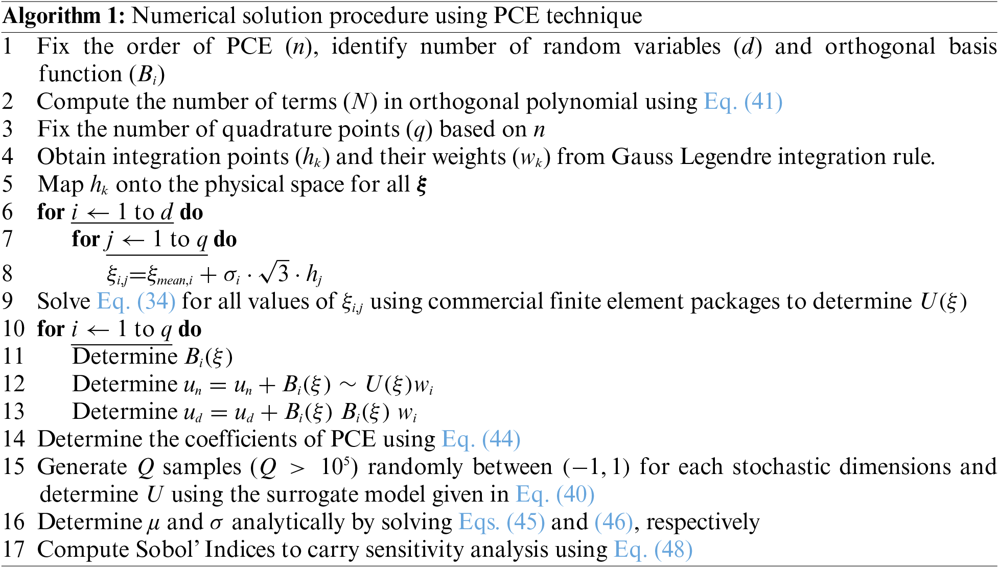
The number of terms in Eq. (40) (including the zeroth order term) can be computed using the equation given below:

N=(n+d)!n!d!(41)

where n is the order of PCE. Higher PCE orders will increase terms in Eq. (40) and improve the solution accuracy. The penalty is the increased computational cost. Eq. (40) can be rewritten as

⟨U(ξ),Bi(ξ)⟩=⟨∑i=1Nuj Bj(ξ),Bi(ξ)⟩(42)

Applying the orthogonality of the polynomial function (Eq. (39)):

⟨U(ξ),Bi(ξ)⟩=ui⟨Bi(ξ)⟩2(43)

The coefficients of the polynomial are given by the expression:

ui=⟨U(ξ),Bi(ξ)⟩⟨Bi(ξ)⟩2(44)

The above equation can be solved using standard integration approaches such as the Gaussian quadrature rule. The number of integration points (q) used for integration depends upon the order of polynomials. The mean (μ) of the dependent variable is

μ=u0(45)

The standard deviation (σ) of the dependent variable is

σ=∑i=1Nui2⟨Bi(ξ),Bi(ξ)⟩(46)

Variance (V) is defined as σ2. Variance of the dependent variable can be expressed as

V=∑i=1Nui2⟨Bi(ξ)Bi(ξ)⟩(47)

Global sensitivity analysis can be carried out by determining the Sobol’s Indices, SiT. Sobol’s indices are computed from the Fourier coefficients and give the sensitivity of each RV on the system’s dependent variable of interest. Thus, the sensitivity computation is done by post-processing the Fourier coefficients without additional computational cost. The higher the numerical value of Sobol’s Indices, the more sensitivity. The analytically expression for computing Sobol Indices is

SiT=∑j∈IiTuj2V(48)

where IiT is defined as

IiT={J∈N:ji>0}(49)

Fig. 2 gives a schematic representation of PCE implementation for modelling fatigue phase-field having multiple independent RVs. The technique can be classified into three phases: Phase 1: Pre-processing, Phase 2: Processing phase, and Phase 3: Post-Processing. In the pre-processing step, simulation points (quadrature points) are determined. The number of simulation points (black dots) depends on the PCE order and d. In the processing phase, fatigue phase-field simulations are run for each simulation point specified in the pre-processing to obtain the dependent variable response. In the post-processing phase, the results are used to determine the Fourier coefficients, SiT, μ, σ and PDF of the dependent variable. Detailed implementation algorithm is given in Algortihm 1.

Figure 2: Schematic representation of stochastic analysis of fatigue phase-field using non-intrusive polynomial chaos technique

5  Results and Discussion

In this section, it is proposed to apply and compare PCE technique using certain numerical experiments. Results obtained are compared against MCS and deterministic responses wherever possible. CPU hours required for simulating a SNS under symmetric cyclic axial load is 14.5 CPU hrs (approx.) [70]. Therefore, MCS runs for real-life problems are compute-intensive due to the large DOF required to model complex geometry. For such problems, MCS runs can extend for months or even years, given the considerable number of sample runs required, which can reach 105 or more.

A single element under monotonic loading is chosen to validate the results of the PCE technique with MCS runs in Section 5.1. Peak failure load is treated as the dependent variable of interest for this numerical problem. In subsequent sections (Sections 5.2 to 5.5), fatigue fracture responses of brittle specimens are studied to demonstrate the application of the proposed stochastic approach. Nf is the dependent variable of interest for all subsequent studies. The μ, σ, minimum and maximum responses are determined for the randomness in geometry and material properties. All simulations in subsequent sections are carried out in plane strain conditions and displacement control loading unless otherwise specified. Four node iso-parametric quadrilateral elements are employed for idealizing the geometry. All RVs are assumed to follow uniform distribution unless otherwise stated. Mesh convergence studies were carried out for all the simulations. However, for the brevity of the paper, convergence results are not discussed in detail.

The numerical simulations were carried out using ABAQUS® on a 32 GB RAM machine with Intel® Xeon® Gold 5118 CPU @ 2.30 GHz (2 Processors). The solutions from ABAQUS® are post-processed using MATLAB® to determine the system responses.

5.1 Homogeneous Plane Strain Plate under Uniaxial Tension

To compare the results of the PCE technique with MCS runs, a benchmark problem of 2D plane strain plate under uniaxial tension is considered [58,59,76]. Material properties of the specimen and ℓo chosen for the simulation are listed in Table 1 [76]. Geometry (w = 1 mm) and boundary condition of the specimen is given in Fig. 3 [76]. The specimen is modelled as a single four-node iso-parametric quadrilateral element. A single-element problem is chosen to validate the results of the PCE technique with MCS runs. The uniaxial tension is applied as a displacement load of u = 0.1×w at the CD edge. Load is applied in increments of δu = 10−4×w. The load-carrying capacity of the specimen decreases as displacement load is incrementally applied on the specimen and ϕ grows from an intact state (ϕ=0) to a fully damaged state (ϕ=1).

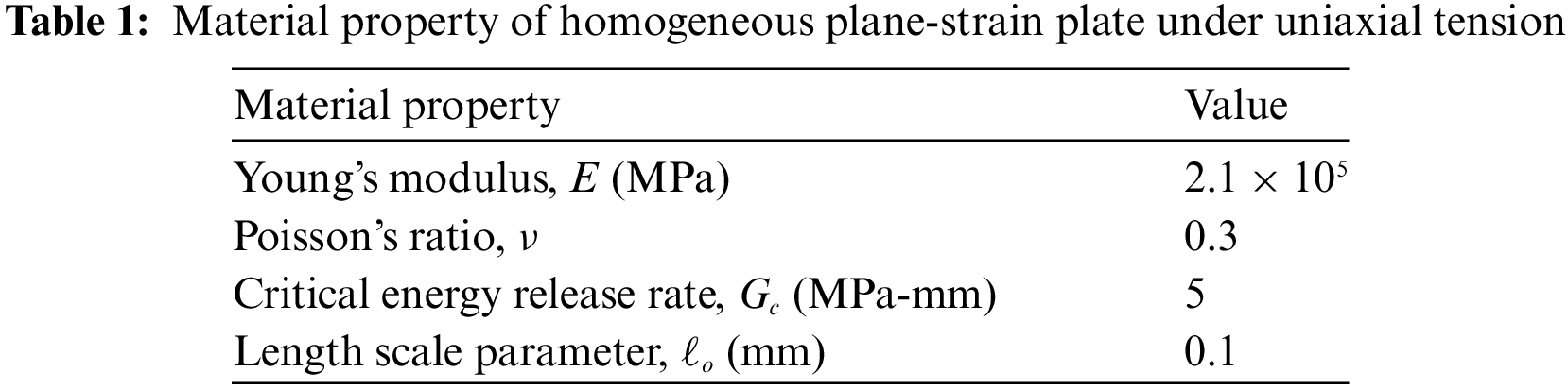
Figure 3: Geometry and boundary condition of homogeneous plane-strain plate under uniaxial tension

Three material properties are considered to be independent RVs for this study: (E, Gc and ν). Table 2 gives the coefficient of variation (CoV) for these independent random variables for the three case studies considered in this section. For Case 1 material distribution, Young’s Modulus (E) alone is treated as the random independent variable and is assumed to have CoV of 0.2. For Case 2 material distribution, CoV of E and Gc are 0.2 and 0.15, respectively. For Case 3 material distribution, in addition to the RVs in Case 2, Poisson’s ratio (ν) is assumed to have a CoV of 0.1. Peak reaction load is treated as the dependent variable of interest. For detailed insights into analytical solutions and implementation of PFM for this specific problem, readers are requested to refer to [59,76]. A total of 2×105 simulation runs are carried out for each distribution case to obtain a converged MCS solution. The μ and σ for MCS and PCE runs are listed in Table 2. PCE functions of orders 1, 2 and 3 are used for simulations. μ and σ of peak reaction load determined using PCE runs are compared with that of MCS runs. From the results, it can be observed that the PCE results are comparable to MCS results. Second and third PCE orders can approximate the results better. The PDF for the peak reaction load determined using MCS and PCE runs are compared in Fig. 4 for all three material distribution cases. From Fig. 4 and Table 2, it can be observed that the second and third PCE orders are in good agreement with MCS runs. For Case 3 material gradation with PCE order 3, 64 simulation runs were carried out. Thus, PCE simulations can obtain probabilistic measures of the dependent variables of interest with good estimates using a significantly lower number of simulation runs. Total sensitivity analysis is carried out for the RVs considered for all three gradation cases using PCE coefficients. Sobol’ indices for the sensitivity analysis are given in Fig. 5. A good agreement is observed between the obtained results in Fig. 5a and [58]. Analyzing Fig. 5b, E influences the peak load carrying capacity of the specimen the most in comparison to Gc and ν. Mean, maximum and minimum plots of reaction load vs. applied displacement using PCE technique and MCS runs are plotted in Fig. 6. Results of the third-order PCE technique are used to obtain the bounds of response. The mean, maximum, and minimum responses obtained using the PCE technique match with MCS.

Figure 4: Probability density function of peak reaction load (N) for a homogeneous plane-strain plate under uniaxial tension from PCE and MCS results: (a) Case 1 material distribution (b) Case 2 material distribution (c) Case 3 material distribution

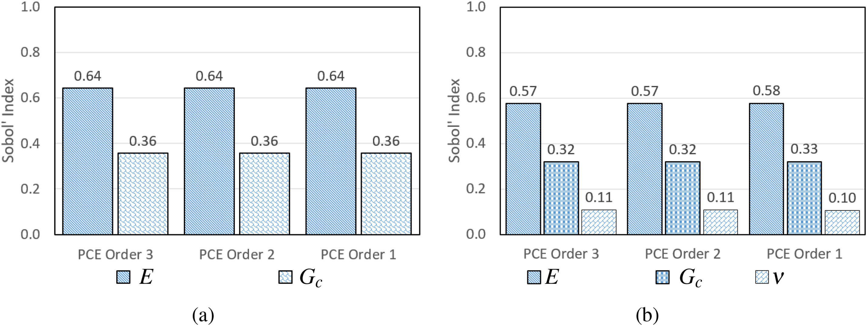
Figure 5: Total sensitivity analysis using Sobol’ Indices for a homogeneous plane-strain plate under uniaxial tension using PCE of orders 1, 2 and 3: (a) Case 2 material distribution (b) Case 3 material distribution

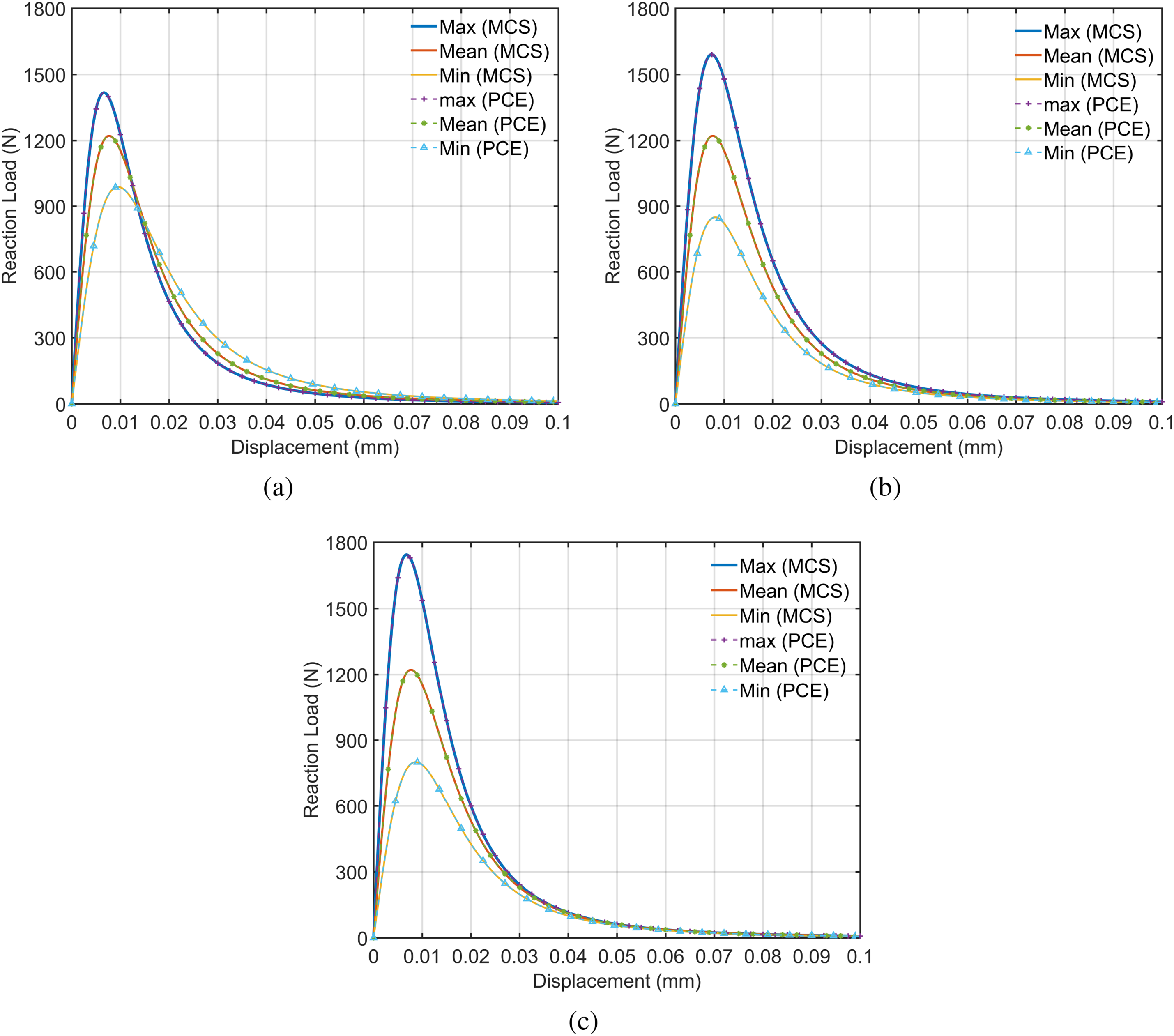
Figure 6: Load vs. displacement plots for a homogeneous plane-strain plate under uniaxial tension from PCE and MCS results: (a) Case 1 material distribution (b) Case 2 material distribution (c) Case 3 material distribution

5.2 Uniaxial Tension-Compression Study in a SNS

This section studies fracture response for a SNS [62,67,77] subjected to symmetric cyclic load. This common benchmark problem can be considered as simulating the conditions experienced by a test coupon subjected to uniform straining in an axial direction. Material properties for the simulations are tabulated in Table 3 [45]. The geometry and boundary conditions are given in Fig. 7 (w = 1 mm) [45]. The nodes corresponding to edge AB are constrained in Y directions and the node at corner A are constrained in both X and Y direction. The specimen is subjected to a quasi-static cyclic displacement load along edge CD with load ratio, R = −1 as shown in Fig. 8 and Δu=4×10−3 mm. The amplitude of the applied displacement load in this section and subsequent sections are considered to simulate Low cycle (LC) fatigue applications. The specimen undergoes Model I fracture. The minimum characteristic element size (h) in the crack growth zone is maintained at least 16 times ℓo to ensure sufficient mesh refinement [78]. The model contains approximately 2.2×105 DOF. Fig. 9a gives the relationship between crack length a and the number of cycles N. The result is consistent with [45,70]. Simulated crack evolution is given in Fig. 9b. For this study, two different material distribution cases are explored. E and Gc are treated as RVs of interest. For Case 1 material distribution, E alone is treated as the RV with CoV of 0.1. For Case 2, both E and Gc are assumed to have a CoV of 0.1 and 0.05, respectively. The CoVs for all cases are tabulated in Table 4. Lower and upper bounds of responses obtained by carrying out deterministic runs are given in Table 4. PDF for Nf for the first three PCE orders is given in Fig. 10 for Case 1 and Case 2. From the figure, it can be observed that PDFs of PCE of orders 2 and 3 coincide showing converged results. The μ, σ, minimum and maximum responses for Case 1 and Case 2 material distributions are tabulated in Table 4. Mean, minimum and maximum responses are compared with deterministic responses. Second and third PCE orders can better approximate the results and display a converged solution. αT is dependent on the value of Gc [45] and hence not chosen as an independent random material property variable for this study and subsequent studies. Total sensitivity analysis is carried out using third-order PCE coefficients and is given in Fig. 11. E and Gc are found to influence the Nf; however E is still the governing parameter. The minimum, mean and maximum response for crack length vs. the number of cycles for Case 1 and Case 2 material randomness is given in Fig. 12.

Figure 7: Boundary and geometry of SNS

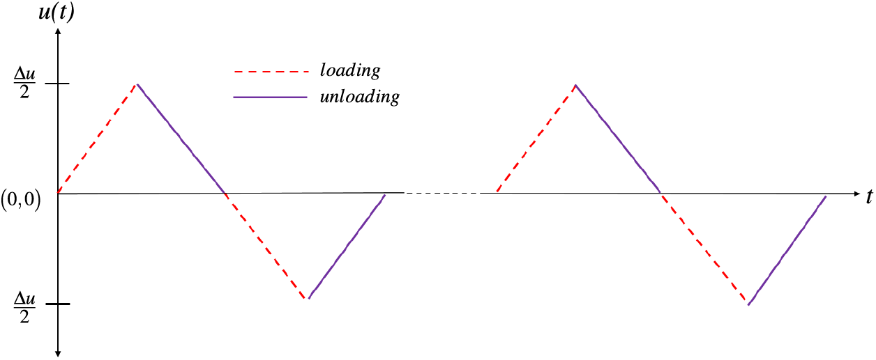
Figure 8: Piece-wise linear loading cycle

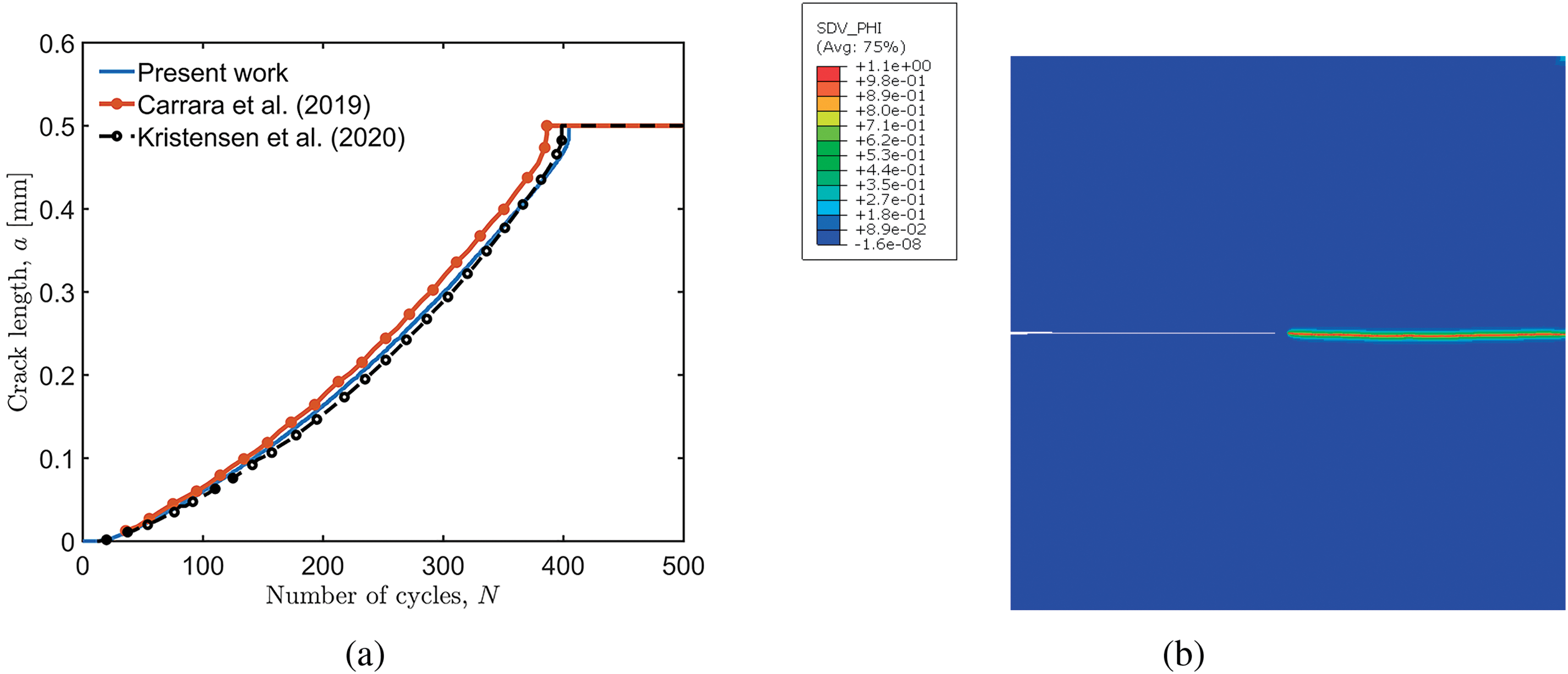
Figure 9: SNS under symmetric cyclic axial load (a) Crack length a vs. number of cycles N (b) Phase-field plot [22,45]

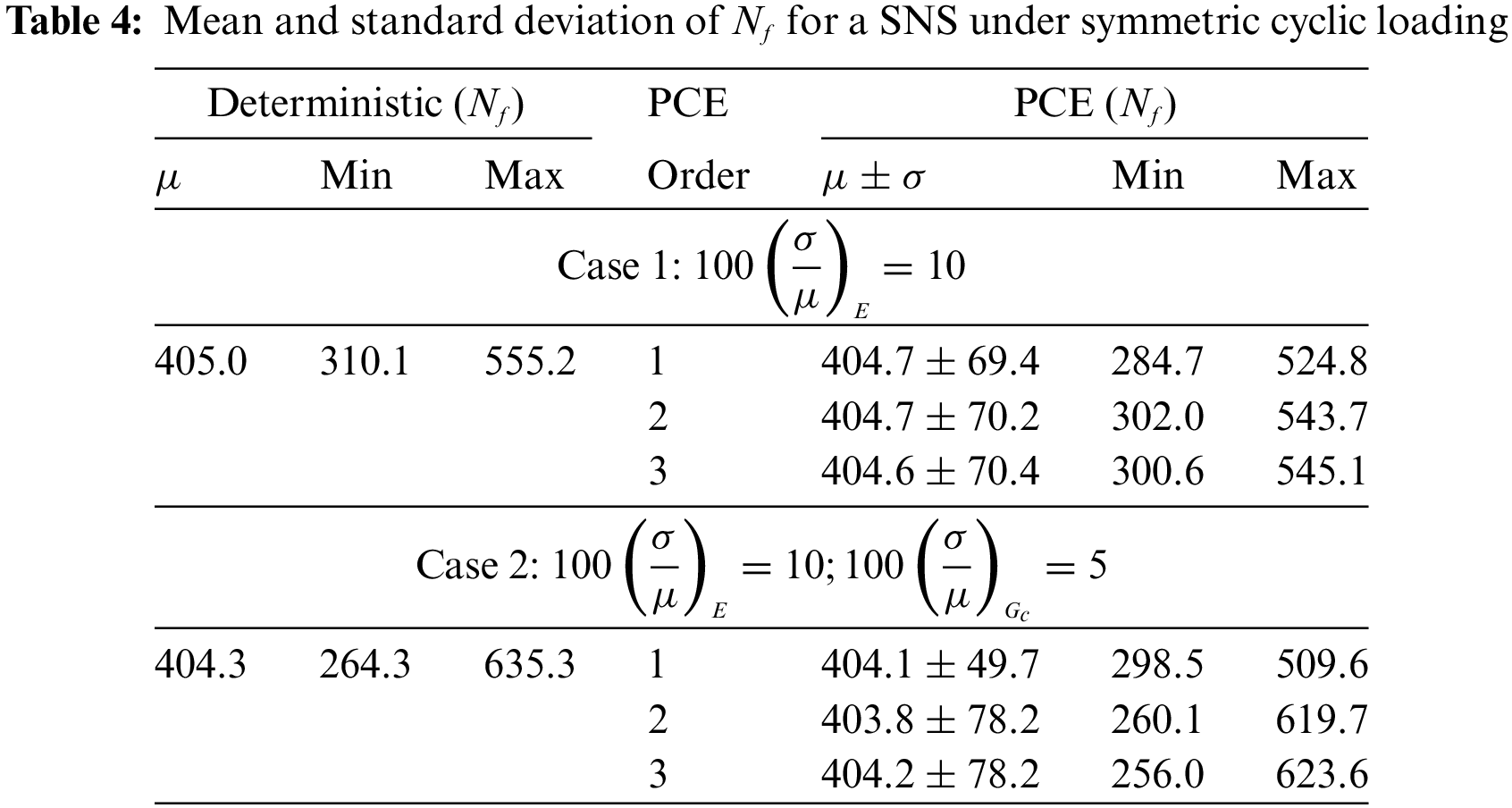
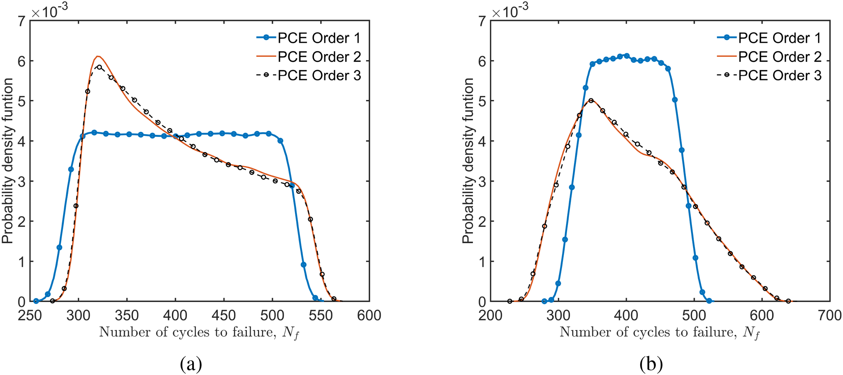
Figure 10: Probability density function of Nf for a SNS under symmetric cyclic loading using PCE of orders of 1, 2 and 3 (a) Case 1 material distribution (b) Case 2 material distribution

Figure 11: Total sensitivity analysis using Sobol’ Indices for SNS under symmetric cyclic axial loading using PCE of order 3 for Case 2 material distribution

Figure 12: Crack length vs. the number of cycles for a SNS under symmetric cyclic loading (a) Case 1 material distribution (b) Case 2 material distribution

5.3 Notched Beam under Asymmetric Three-Point Bending

Fatigue crack propagation is studied for a notched beam subjected to an asymmetric three-point bending load. Material properties are identical to Section 5.2. The geometry of the specimen (w = 2 mm) along with boundary conditions is given in Fig. 13. ℓo and αT for the specimen are 0.04 mm and 5.625 MPa, respectively. The model is discretized with approximately 55,000 DOF. A non-inverting cyclic displacement load is applied with amplitude Δu = 0.0125 mm (Fig. 14). The specimen undergoes Mode I fracture when the displacement load is applied directly above the notch. In this section, load is applied at an offset from the notch axis to simulate mixed-mode fracture ie Mode I + Mode II fracture. Mode II component can be increased by moving the load away from the notch. For numerical discussion, we treat E and Gc as two random independent material properties having CoV of 8% each. In this study, the dependent variable of interest is the number of cycles (Nf) required for the crack to grow from the notch tip to 0.6w in the Y direction. Phase-field plot for the nominal case is given in Fig. 15. PDF of Nf using PCE of first, second and third orders are given in Fig. 16a. Analysing the figure, second- and third-order PDFs match closely, indicating convergence. The μ and σ of the dependent variable for PCE simulations are listed in Table 5. The sensitivity analysis is carried out for all the PCE orders and computed Sobol’ Indices are given in Fig. 16b. From the figure, it can be concluded that E and Gc are equally sensitive and influence the system’s response. Mean, upper and lower bounds of a vs. N due to material randomness are given in Fig. 17.

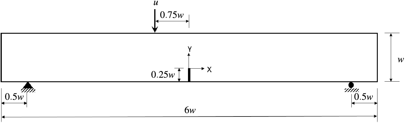
Figure 13: Geometry and boundary condition of notched beam under asymmetric three-point bending

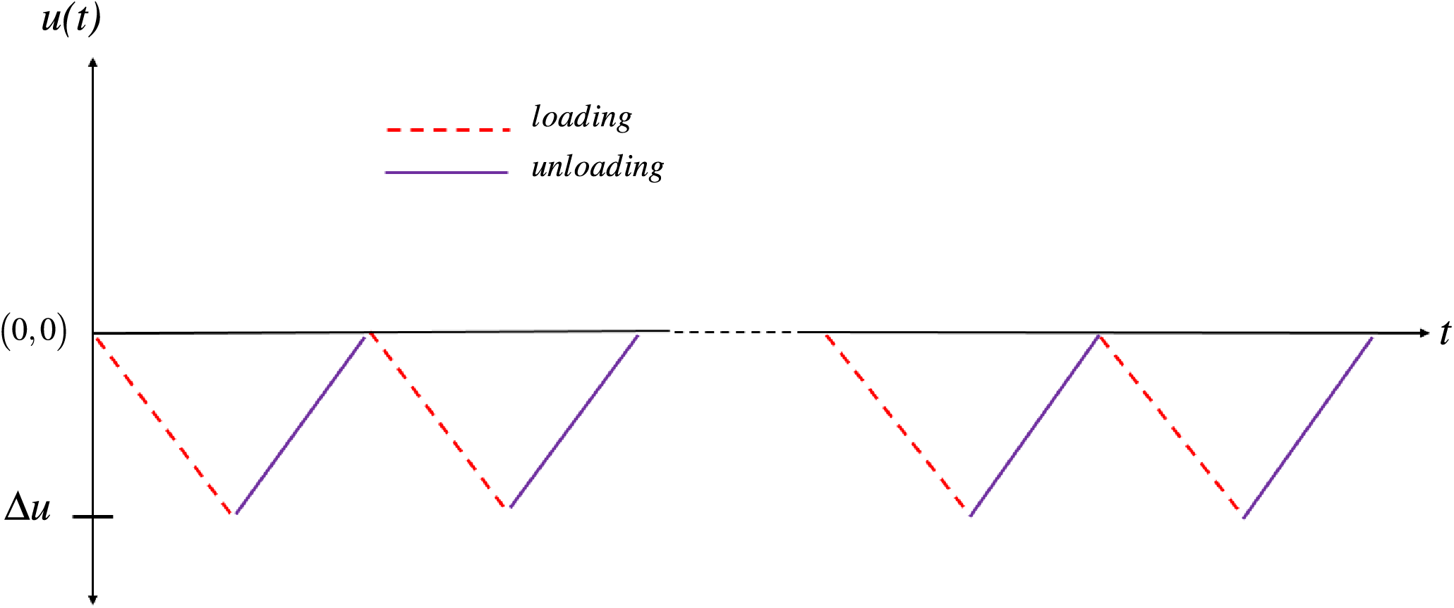
Figure 14: Non inverting cyclic displacement load

Figure 15: Phase-field plot for a notched beam under asymmetric three-point bending under non-inverting cyclic loading

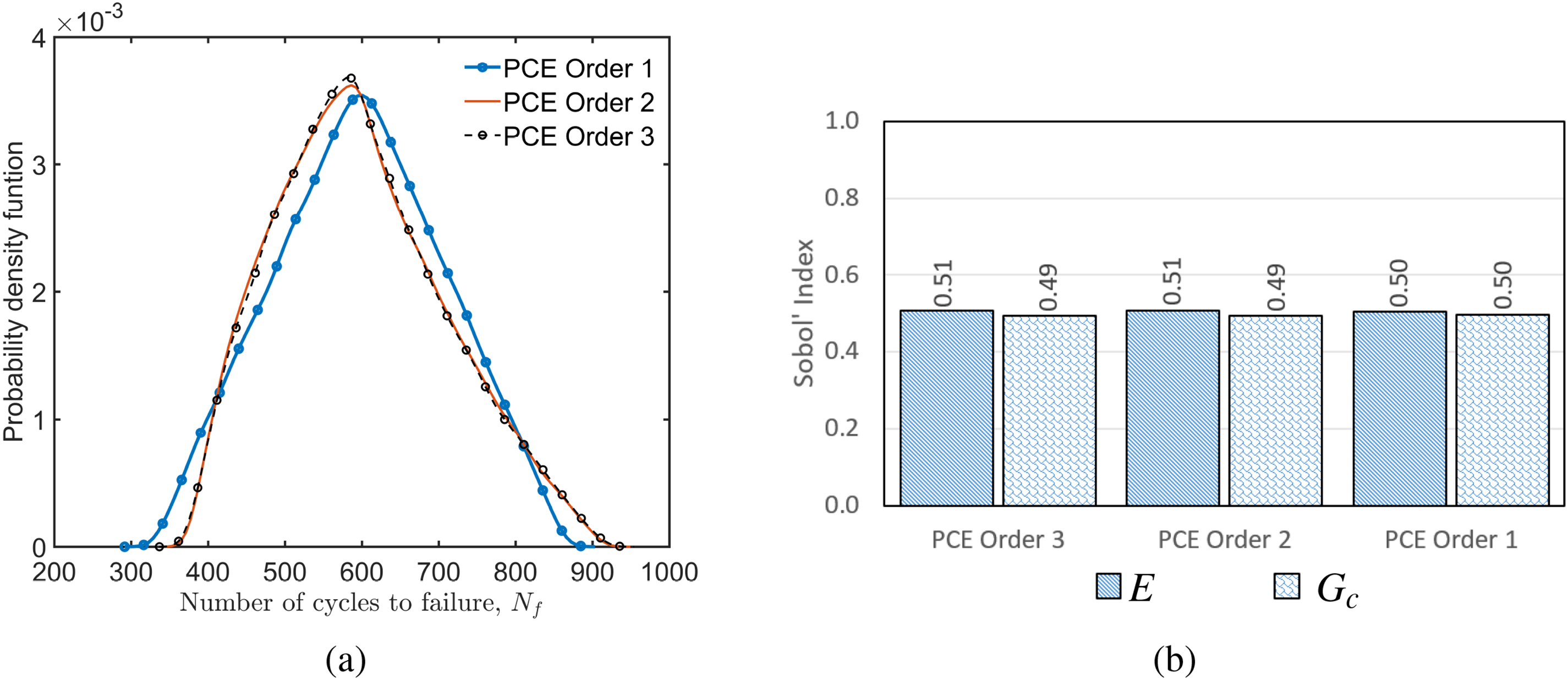
Figure 16: Fatigue crack growth in a notched beam under asymmetric three-point bending under non-inverting cyclic loading (a) Probability density function of Nf (b) Total sensitivity analysis using Sobol’ Indices

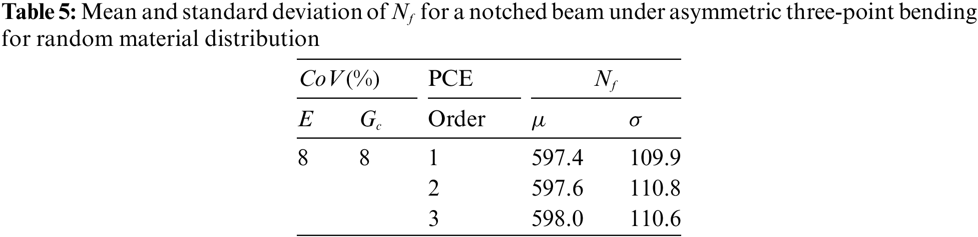
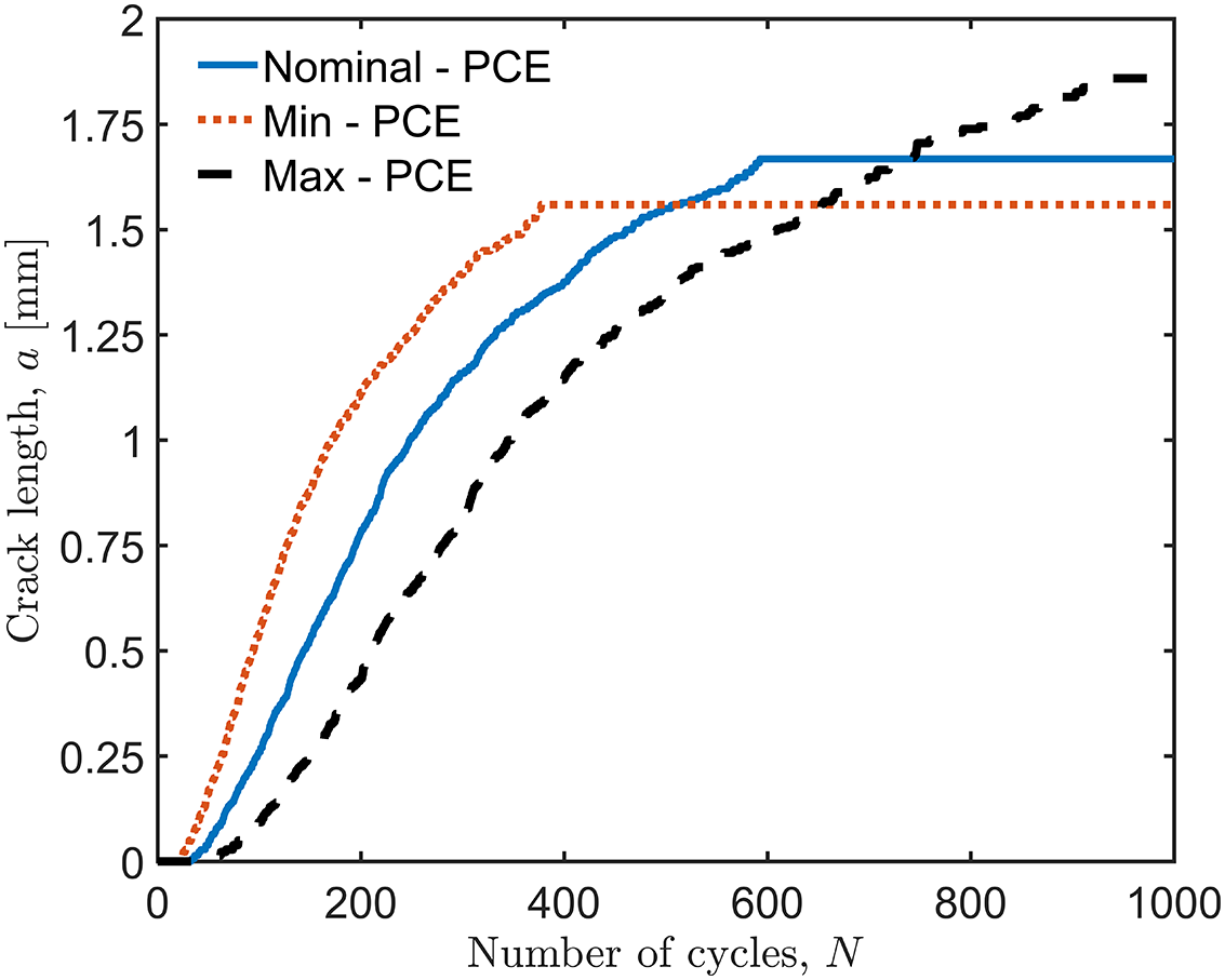
Figure 17: Crack length vs. the number of cycles for a notched beam under asymmetric three-point bending under non-inverting cyclic loading

5.4 Fatigue Growth in a Compact-Tension (CT) Test Specimen

This section considers fatigue crack growth in a CT test specimen. The geometry and boundary conditions of the specimen are given in Fig. 18a. Material properties of the specimen are tabulated in Table 6 [74]. The specimen is subjected to symmetric cyclic displacement load as shown in Fig. 8 with Δu = 0.13 mm. The finite element discretization and statistics are given in Fig. 18b. The element density is increased with h = 15×ℓo in the crack growth zone. For this discussion, we consider two material properties (E and Gc) and one geometric parameter (Cl) as the random independent variables. The CoV for E, Gc, Cl are assumed to be 0.08, 0.04 and 0.05, respectively. Studies are carried out using PCE functions of order one, two and three. Table 7 lists the μ and σ of Nf using PCE of order up to three. Phase-field plot for the simulation with nominal value is given in Fig. 19. PDF of Nf is given in Fig. 20. PCE of order two and above are required to capture the response for the RV distribution studied in this section. Hence, it is recommended to analyze using higher-order PCE until convergence is obtained. Global sensitivity analysis is performed to determine the sensitive parameter influencing Nf using Sobol’ indices. E is found to be the most sensitive parameter while the sensitivity of response due to randomness of Cl is negligibly small. Sobol’ indices for the distribution cases are given in Fig. 21. The mean and extreme responses for the crack growth vs. the number of cycles is given in Fig. 22. The minimum response of the system is obtained for the upper bounds of E and Cl and the lower bound of Gc, and vice versa for the maximum response.

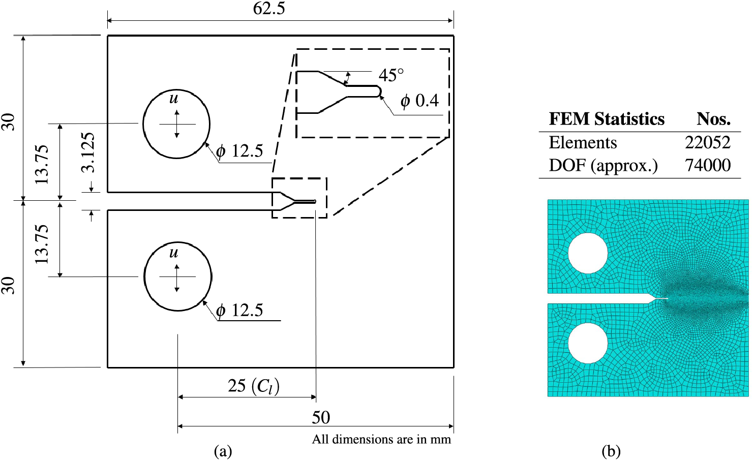
Figure 18: Fatigue crack growth in a CT test specimen (a) Geometry and boundary (b) Finite element discretization and statistics

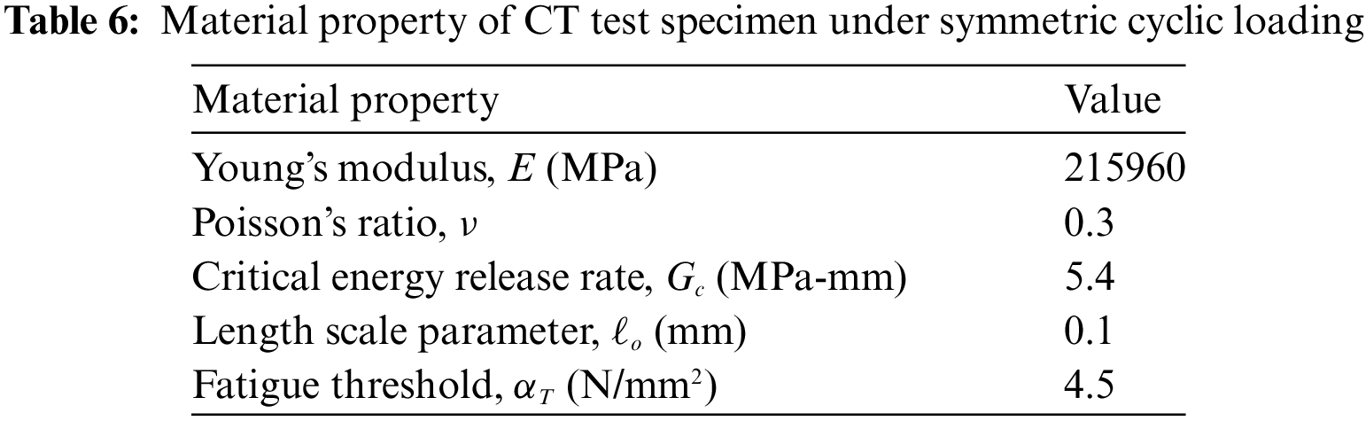
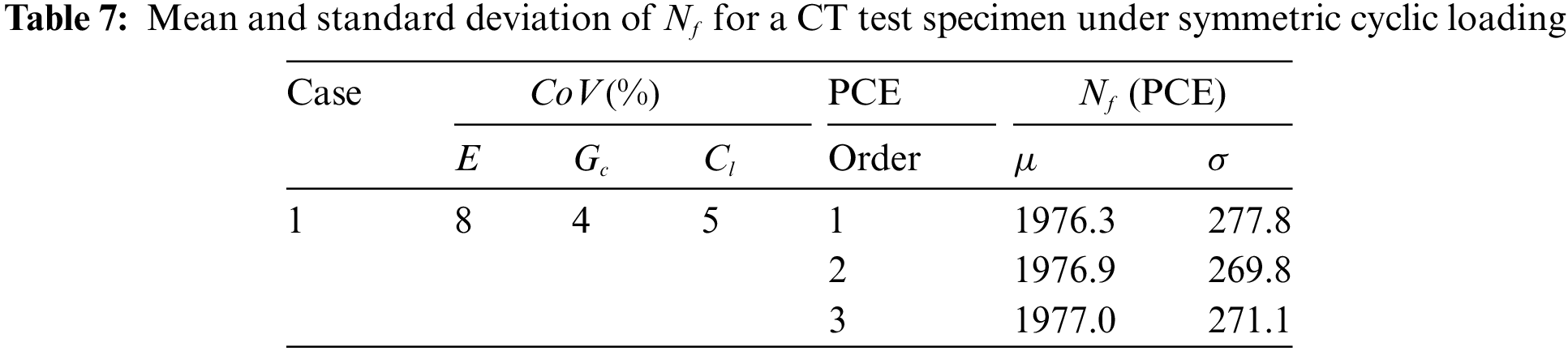
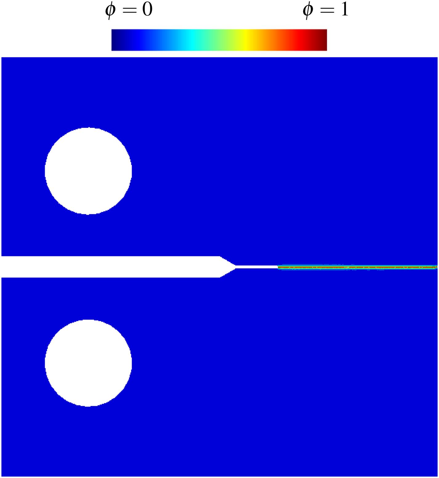
Figure 19: Phase-field plot for a CT test specimen under symmetric cyclic loading

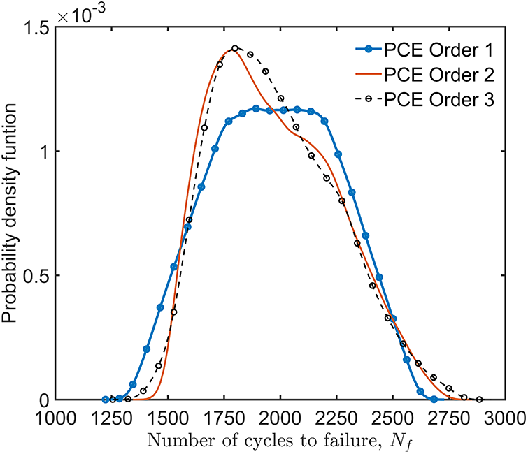
Figure 20: Probability density function of Nf for a CT specimen under symmetric cyclic loading determined using PCE technique

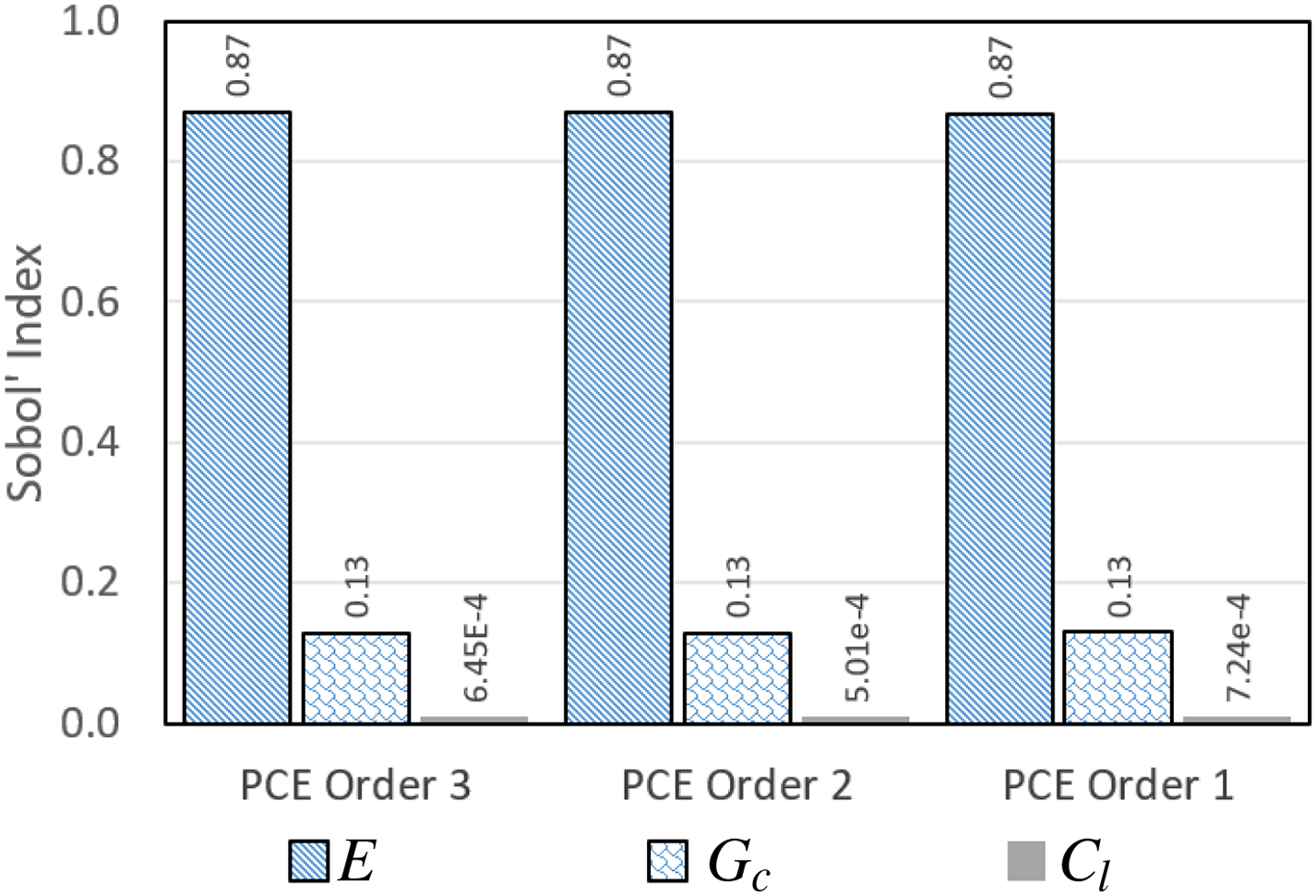
Figure 21: Total sensitivity analysis for a CT specimen under symmetric cyclic loading

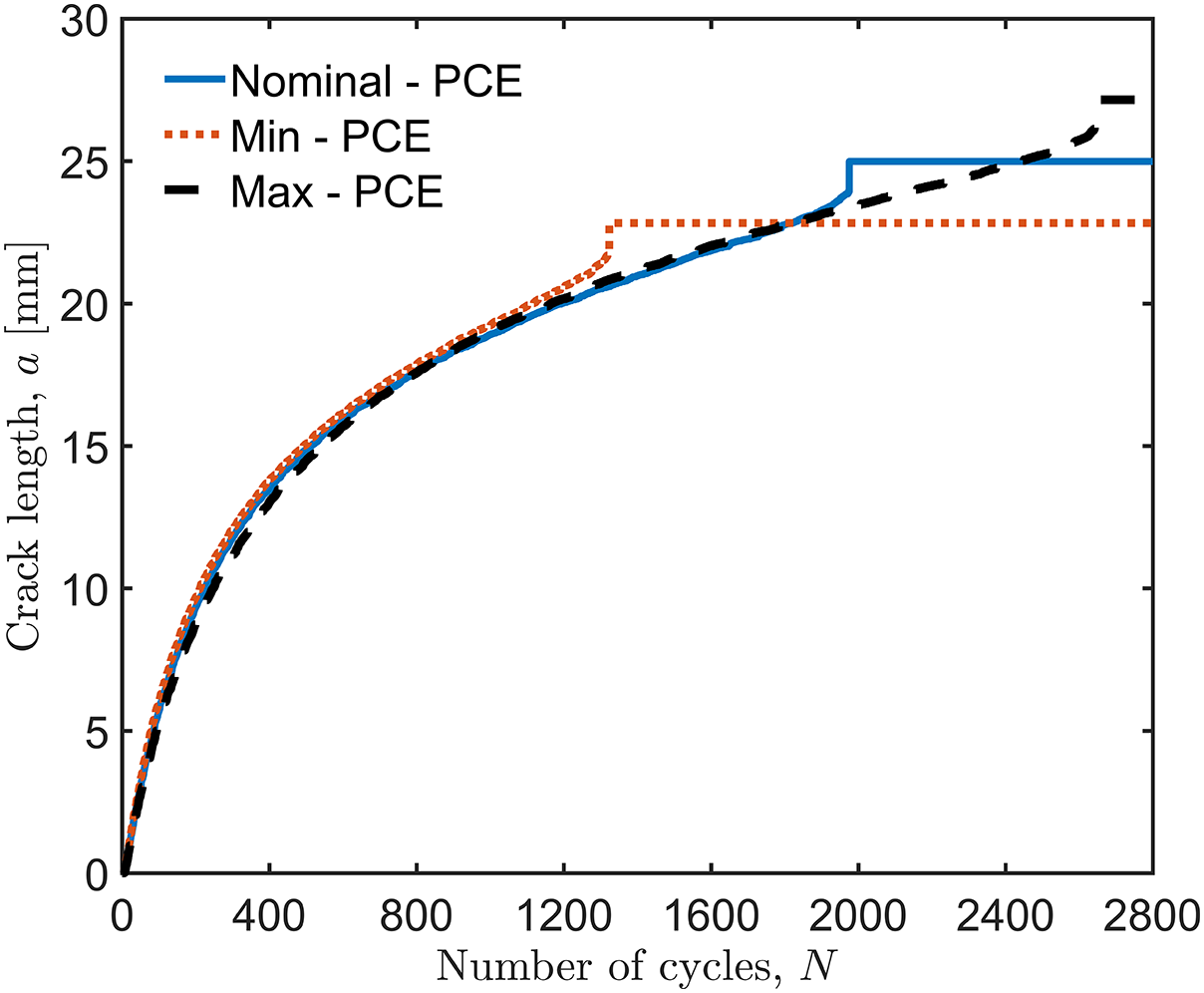
Figure 22: Crack length vs. the number of cycles for a CT test specimen under symmetric cyclic loading

5.5 Fatigue Growth in a Compact-Tension Test Specimen with a Hole

This last section studies fatigue growth for a CT test specimen with a hole adjacent to the crack growth trajectory. The geometry and boundary conditions are given in Fig. 23a. The material properties and applied loads are identical to the specimen studied in Section 5.4. The finite element discretization and statistics are given in Fig. 23b. For this example problem, hole position (hp) and Gc are treated as independent RVs. CoV of these two random independent parameters are tabulated in Table 8. Nf is treated as the dependent variable of interest. Phase-field plot for the nominal run is given in Fig. 24. The predicted PDF of Nf for PCE orders 1, 2 and 3 are given in Fig. 25a. The μ and σ of Nf are computed using the PCE technique for all three orders and are tabulated in Table 8. Studying Fig. 25a and Table 8, it is observed that a PCE order of 1 is sufficient to capture the randomness of Nf. The total sensitivity analysis results are shown in Fig. 25b. It is observed that both Gc and hp are found to influence the distribution of Nf. From the figure, it can be concluded that Gc is found to have a greater influence among the two RVs. Convergence of the total Sobol indices for all PCE orders are given in Fig. 25b. Fig. 26 highlights the minimum, maximum and nominal response for crack length vs. the number of cycles. Fig. 27 gives the crack growth trajectory for the response bounds.

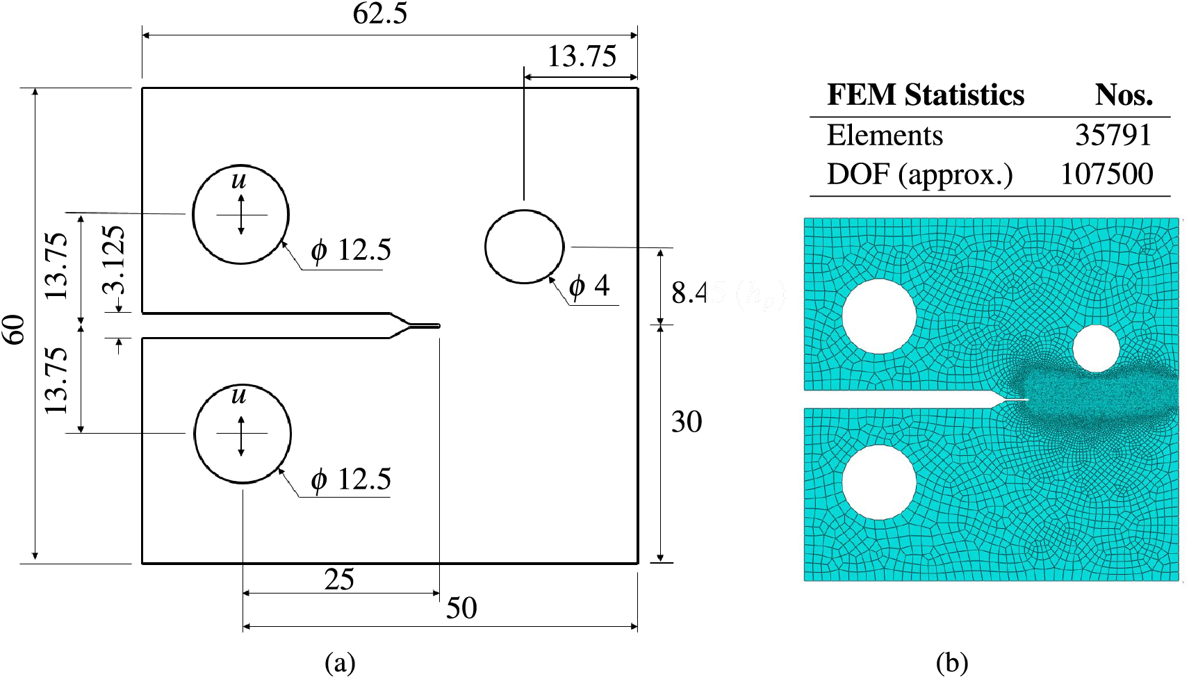
Figure 23: Fatigue crack growth in a CT test specimen with a hole (a) Geometry and boundary (b) Finite element discretization and statistics

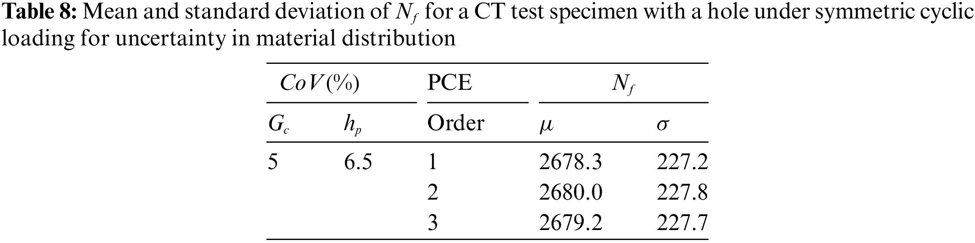
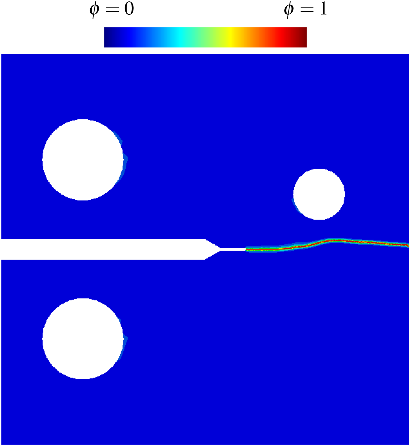
Figure 24: Phase-field plot for a CT test specimen with a hole under symmetric cyclic loading

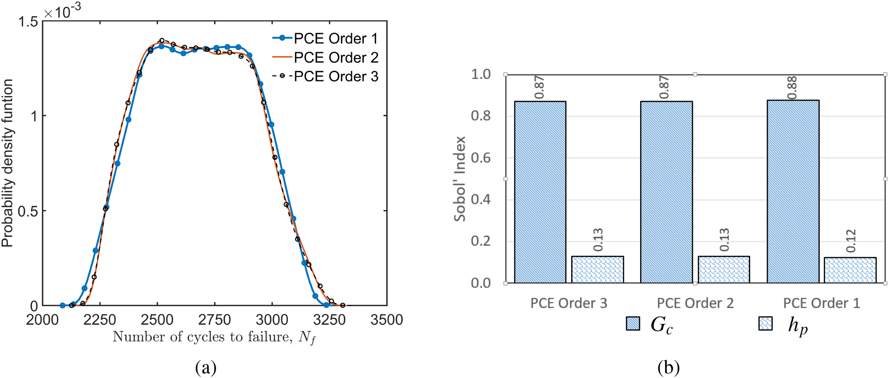
Figure 25: Fatigue crack growth in a CT test specimen with a hole under symmetric cyclic loading (a) Probability density function of Nf (b) Total sensitivity analysis using Sobol’ Indices

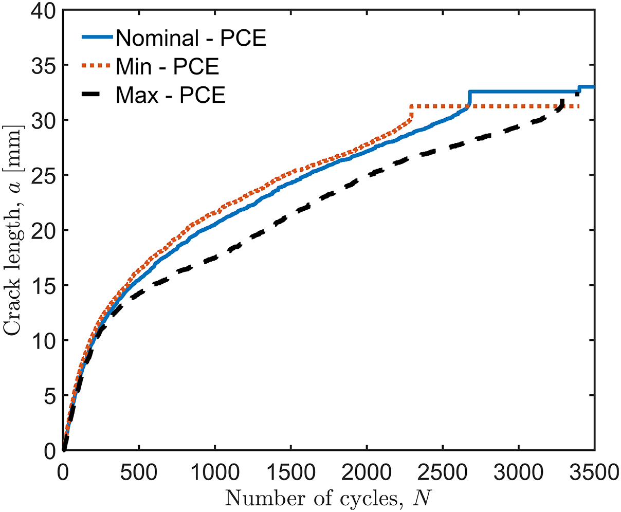
Figure 26: Crack length vs. the number of cycles for a CT test specimen with a hole under symmetric cyclic loading

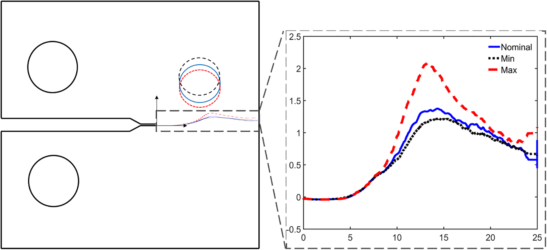
Figure 27: Crack growth path for a CT test specimen with a hole under symmetric cyclic loading

6  Conclusion

In this work, non-intrusive stochastic fatigue fracture studies are carried out on brittle materials when geometric parameters and material properties are random independent variables. Number of cycles to failure is treated as the dependent variable of interest. PCE technique is employed with PFM for fatigue fracture problems and is solved using finite element method. First and second-order stochastic moments of dependent variables and their bounds are determined using PCE of up to three orders. The results obtained are compared with those of MCS and deterministic approaches wherever possible and are in close agreement. PCE approach can achieve the results in significantly fewer simulations than MCS runs where the simulations are computationally expensive. Five different numerical problems are solved to demonstrate the application of the proposed probabilistic technique. This probabilistic approach to fracture problems does not require modification of the existing finite element code and can perform stochastic analysis by direct pre/post-processing. Sensitivity analysis is also carried out using Sobol’ indices to determine the influence of various independent random variables on the system’s responses. Sensitivity studies are carried out by simply post-processing the coefficients of PCE polynomials. PCE faces challenges in accurately representing highly nonlinear systems and discontinuous functions. Despite these limitations, PCE is a valuable uncertainty quantification and sensitivity analysis tool in sensitive applications like aerospace, nuclear and biomedical to assess safety factors without computational overheads.

Acknowledgement: We are thankful for the insightful comments from anonymous reviewers, which have greatly improved this manuscript.

Funding Statement: The authors received no specific funding for this study.

Author Contributions: The authors confirm their contribution to the paper as follows: Original draft: Rajan Aravind;Visualization: Rajan Aravind, Sundararajan Natarajan, Ratna Kumar Annabattula, Krishnankutty Jayakumar; Validation: Rajan Aravind; Methodology: Rajan Aravind, Sundararajan Natarajan, Ratna Kumar Annabattula; Investigation: Rajan Aravind; Formal analysis: Rajan Aravind, Sundararajan Natarajan, Ratna Kumar Annabattula, Krishnankutty Jayakumar; Data curation: Rajan Aravind, Sundararajan Natarajan, Ratna Kumar Annabattula; Conceptualization: Rajan Aravind, Sundararajan Natarajan, Ratna Kumar Annabattula; review & editing: Sundararajan Natarajan, Ratna Kumar Annabattula, Krishnankutty Jayakumar; Supervision: Ratna Kumar Annabattula, Krishnankutty Jayakumar; Project administration: Ratna Kumar Annabattula. All authors reviewed the results and approved the final version of the manuscript.

Availability of Data and Materials: Data will be made available on request.

Ethics Approval: Not applicable.

Conflicts of Interest: The authors declare that they have no conflicts of interest to report regarding the present study.

References

1. Suresh S. Fatigue of materials. 2nd ed. Cambridge: Cambridge University Press; 1998. [Google Scholar]

2. Wohler A. Versuche uber die Festigkeit der Eisenbahnwagenachsen. Zeitschrift fur Bauwesen. 1860;10:160–1. [Google Scholar]

3. Paris PC, Gomez MP, Anderson WEP. A rational analytic theory of fatigue. Trend Eng. 1961;13:9–14. [Google Scholar]

4. Ingraffea AR, Saouma V. Numerical modeling of discrete crack propagation in reinforced and plain concrete. Fract Mech Concr, Struct Appl Numer Calc. 1985;4:171–225. [Google Scholar]

5. Dugdale DS. Yielding of steel sheets containing slits. J Mech Phys Solids. 1960;8(2):100–4. doi:10.1016/0022-5096(60)90013-2. [Google Scholar] [CrossRef]

6. Barenblatt GI. The mathematical theory of equilibrium cracks in brittle fracture. Adv Appl Mech. 1962;7(C):55–129. [Google Scholar]

7. Gravouil A, Moës N, Belytschko T. Non-planar 3D crack growth by the extended finite element and level sets-Part II: level set update. Int J Numer Methods Eng. 2002;53:2569–86. doi:10.1002/nme.v53:11. [Google Scholar] [CrossRef]

8. Rashnooie R, Zeinoddini M, Ahmadpour F, Beheshti Aval SB, Chen T. A coupled XFEM fatigue modelling of crack growth, delamination and bridging in FRP strengthened metallic plates. Eng Fract Mech. 2023;279(2):109017. doi:10.1016/j.engfracmech.2022.109017. [Google Scholar] [CrossRef]

9. Rashid YR. Ultimate strength analysis of prestressed concrete pressure vessels. Nucl Eng Des. 1968;7(4):334–44. doi:10.1016/0029-5493(68)90066-6. [Google Scholar] [CrossRef]

10. Silling SA, Lehoucq RB. Peridynamic theory of solid mechanics. Adv Appl Mech. 2010;44:73–168. doi:10.1016/S0065-2156(10)44002-8. [Google Scholar] [CrossRef]

11. Zhang G, Le Q, Loghin A, Subramaniyan A, Bobaru F. Validation of a peridynamic model for fatigue cracking. Eng Fract Mech. 2016;162(1–2):76–94. doi:10.1016/j.engfracmech.2016.05.008. [Google Scholar] [CrossRef]

12. Collins JB, Levine H. Diffuse interface model of diffusion-limited crystal growth. Phys Rev B. 1985;31(9):6119–22. doi:10.1103/PhysRevB.31.6119. [Google Scholar] [PubMed] [CrossRef]

13. Francfort GA, Marigo JJ. Revisiting brittle fracture as an energy minimization problem. J Mech Phys Solids. 1998;46(8):1319–42. doi:10.1016/S0022-5096(98)00034-9. [Google Scholar] [CrossRef]

14. Griffith AA. The phenomena of rupture and flow in solids. Philos Trans R Soc Lond Ser A. 1921;221:163–98. doi:10.1098/rsta.1921.0006. [Google Scholar] [CrossRef]

15. Bourdin B, Francfort GA, Marigo JJ. The variational approach to fracture. J Elast. 2008;91(1–3):5–148. doi:10.1007/s10659-007-9107-3. [Google Scholar] [CrossRef]

16. Nguyen TT, Réthoré J, Baietto MC. Phase field modelling of anisotropic crack propagation. Eur J Mech—A/Solids. 2017;65(8):279–88. doi:10.1016/j.euromechsol.2017.05.002. [Google Scholar] [CrossRef]

17. Peng F, Huang W, Zhang ZQ, Fu Guo T, Ma YE. Phase field simulation for fracture behavior of hyperelastic material at large deformation based on edge-based smoothed finite element method. Eng Fract Mech. 2020;238(8):107233. doi:10.1016/j.engfracmech.2020.107233. [Google Scholar] [CrossRef]

18. Li P, Li D, Wang Q, Zhou K. Phase-field modeling of hydro-thermally induced fracture in thermo-poroelastic media. Eng Fract Mech. 2021;254(3):107887. doi:10.1016/j.engfracmech.2021.107887. [Google Scholar] [CrossRef]

19. Shen R, Waisman H, Guo L. Fracture of viscoelastic solids modeled with a modified phase field method. Comput Methods Appl Mech Eng. 2019;346:862–90. doi:10.1016/j.cma.2018.09.018. [Google Scholar] [CrossRef]

20. Miehe C, Aldakheel F, Raina A. Phase field modeling of ductile fracture at finite strains: a variational gradient-extended plasticity-damage theory. Int J Plast. 2016;84:1–32. doi:10.1016/j.ijplas.2016.04.011. [Google Scholar] [CrossRef]

21. Hirshikesh, Natarajan S, Annabattula RK, Martínez-Pañeda E. Phase field modelling of crack propagation in functionally graded materials. Compos Part B Eng. 2019;169:239–48. [Google Scholar]

22. Kristensen PK, Niordson CF, Martínez-Pańeda E. A phase field model for elastic-gradient-plastic solids undergoing hydrogen embrittlement. J Mech Phys Solids. 2020;143:104093. doi:10.1016/j.jmps.2020.104093. [Google Scholar] [CrossRef]

23. Cui C, Ma R, Martínez-Pańeda E. A phase field formulation for dissolution-driven stress corrosion cracking. J Mech Phys Solids. 2021;147:104254. doi:10.1016/j.jmps.2020.104254. [Google Scholar] [CrossRef]

24. Li D, Li P, Li W, Li W, Zhou K. Three-dimensional phase-field modeling of temperature-dependent thermal shock-induced fracture in ceramic materials. Eng Fract Mech. 2022;268:108444. doi:10.1016/j.engfracmech.2022.108444. [Google Scholar] [CrossRef]

25. Mohanty S, Kumbhar PY, Swaminathan N, Annabattula R. A phase-field model for crack growth in electro-mechanically coupled functionally graded piezo ceramics. Smart Mater Struct. 2020;29:045005. doi:10.1088/1361-665X/ab7145. [Google Scholar] [CrossRef]

26. Tan Y, He Y, Li X, Kang G. A phase field model for fatigue fracture in piezoelectric solids: a residual controlled staggered scheme. Comput Methods Appl Mech Eng. 2022;399:115459. doi:10.1016/j.cma.2022.115459. [Google Scholar] [CrossRef]

27. Spetz A, Denzer R, Tudisco E, Dahlblom O. Phase-field fracture modelling of crack nucleation and propagation in porous rock. Int J Fract. 2020;224(1):31–46. doi:10.1007/s10704-020-00444-4. [Google Scholar] [CrossRef]

28. Raina A, Miehe C. A phase-field model for fracture in biological tissues. Biomech Model Mechanobiol. 2016;15(3):479–96. doi:10.1007/s10237-015-0702-0. [Google Scholar] [PubMed] [CrossRef]

29. Wu JY, Nguyen VP, Nguyen CT, Sutula D, Sinaie S, Bordas SPA. Phase-field modeling of fracture. Adv Appl Mech. 2020;53(2):1–183. doi:10.1016/bs.aams.2019.08.001. [Google Scholar] [CrossRef]

30. Yang ZJ, Li BB, Wu JY. X-ray computed tomography images based phase-field modeling of mesoscopic failure in concrete. Eng Fract Mech. 2019;208(4):151–70. doi:10.1016/j.engfracmech.2019.01.005. [Google Scholar] [CrossRef]

31. Konica S, Sain T. A reaction-driven evolving network theory coupled with phase-field fracture to model polymer oxidative aging. J Mech Phys Solids. 2021;150(2):104347. doi:10.1016/j.jmps.2021.104347. [Google Scholar] [CrossRef]

32. Bui TQ, Hu X. A review of phase-field models, fundamentals and their applications to composite laminates. Eng Fract Mech. 2021;248(8):107705. doi:10.1016/j.engfracmech.2021.107705. [Google Scholar] [CrossRef]

33. Ren HL, Zhuang XY, Anitescu C, Rabczuk T. An explicit phase field method for brittle dynamic fracture. Comput Struct. 2019;217:45–56. doi:10.1016/j.compstruc.2019.03.005. [Google Scholar] [CrossRef]

34. Nguyen VP, Wu JY. Modeling dynamic fracture of solids with a phase-field regularized cohesive zone model. Comput Methods Appl Mech Eng. 2018;340:1000–22. doi:10.1016/j.cma.2018.06.015. [Google Scholar] [CrossRef]

35. Schlüter A, Kuhn C, Müller R, Tomut M, Trautmann C, Weick H, et al. Phase field modelling of dynamic thermal fracture in the context of irradiation damage. Contin Mech Thermodyn. 2017;29(4):977–88. doi:10.1007/s00161-015-0456-z. [Google Scholar] [CrossRef]

36. Chukwudozie C, Bourdin B, Yoshioka K. A variational phase-field model for hydraulic fracturing in porous media. Comput Methods Appl Mech Eng. 2019;347:957–82. doi:10.1016/j.cma.2018.12.037. [Google Scholar] [CrossRef]

37. Zhou S, Zhuang X, Rabczuk T. Phase field modeling of brittle compressive-shear fractures in rock-like materials: a new driving force and a hybrid formulation. Comput Methods Appl Mech Eng. 2019;355: 729–52. doi:10.1016/j.cma.2019.06.021. [Google Scholar] [CrossRef]

38. Boldrini JL, Barros de Moraes EA, Chiarelli LR, Fumes FG, Bittencourt ML. A non-isothermal thermodynamically consistent phase field framework for structural damage and fatigue. Comput Methods Appl Mech Eng. 2016;312:395–427. doi:10.1016/j.cma.2016.08.030. [Google Scholar] [CrossRef]

39. Alessi R, Vidoli S, De Lorenzis L. A phenomenological approach to fatigue with a variational phase-field model: the one-dimensional case. Eng Fract Mech. 2018;190:53–73. [Google Scholar]

40. Mesgarnejad A, Imanian A, Karma A. Phase-field models for fatigue crack growth. Theor Appl Fract Mech. 2019;103:102282. doi:10.1016/j.tafmec.2019.102282. [Google Scholar] [CrossRef]

41. Grossman-Ponemon BE, Mesgarnejad A, Karma A. Phase-field modeling of continuous fatigue via toughness degradation. Eng Fract Mech. 2022;264:108255. doi:10.1016/j.engfracmech.2022.108255. [Google Scholar] [CrossRef]

42. Lo YS, Borden M, Ravi-Chandar K, Landis C. A phase-field model for fatigue crack growth. J Mech Phys Solids. 2019;132:103684. doi:10.1016/j.jmps.2019.103684. [Google Scholar] [CrossRef]

43. Caputo M, Fabrizio M. Damage and fatigue described by a fractional derivative model. J Comput Phys. 2015;293:400–8. doi:10.1016/j.jcp.2014.11.012. [Google Scholar] [CrossRef]

44. Amendola G, Fabrizio M, Golden JM. Thermomechanics of damage and fatigue by a phase field model. J Therm Stress. 2016;39(5):487–99. doi:10.1080/01495739.2016.1152140. [Google Scholar] [CrossRef]

45. Carrara P, Ambati M, Alessi R, De Lorenzis L. A framework to model the fatigue behavior of brittle materials based on a variational phase-field approach. Comput Methods Appl Mech Eng. 2020;361:112731. doi:10.1016/j.cma.2019.112731. [Google Scholar] [CrossRef]

46. Ulloa J, Wambacq J, Alessi R, Degrande G, François S. Phase-field modeling of fatigue coupled to cyclic plasticity in an energetic formulation. Comput Methods Appl Mech Eng. 2021;373(2):113473. doi:10.1016/j.cma.2020.113473. [Google Scholar] [CrossRef]

47. Schreiber C, Kuhn C, Muller R, Zohdi T. A phase field modeling approach of cyclic fatigue crack growth. Int J Fract. 2020;225(1):89–100. doi:10.1007/s10704-020-00468-w. [Google Scholar] [CrossRef]

48. Hasan MM, Baxevanis T. A phase-field model for low-cycle fatigue of brittle materials. Int J Fatigue. 2021;150:106297. doi:10.1016/j.ijfatigue.2021.106297. [Google Scholar] [CrossRef]

49. Baktheer A, Martínez-Pañeda E, Aldakheel F. Phase field cohesive zone modeling for fatigue crack propagation in quasi-brittle materials. Comput Methods Appl Mech Eng. 2024;422(4):116834. doi:10.1016/j.cma.2024.116834. [Google Scholar] [CrossRef]

50. Raynaud P, Kirk M, Benson M, Homiack M. Important aspects of probabilistic fracture mechanics analyses. Rockville, MD: United States Nuclear Regulatory Commission; 2018. Available from: https://www.nrc.gov/docs/ML1817/ML18178A431.pdf. [Accessed 2024]. [Google Scholar]

51. Rice JA. Mathematical statistics and data analysis. 3rd ed. Belmont, CA: Thomson/Brooks/Cole; 2007. [Google Scholar]

52. Kaminski M. The stochastic perturbation method for computational mechanics. West Sussex, UK: John Wiley & Sons; 2013. [Google Scholar]

53. Smith RC. Uncertainty quantification: theory, implementation, and applications. Philadelphia: SIAM; 2013. vol. 12. [Google Scholar]

54. Norbert W. The homogeneous chaos. Am J Math. 1938;60(4):897–936. doi:10.2307/2371268. [Google Scholar] [CrossRef]

55. Dinescu C, Smirnov S, Hirsch C, Lacor C. Assessment of intrusive and non-intrusive non-deterministic CFD methodologies based on polynomial chaos expansions. Int J Eng Syst Model Simul. 2010;2(1–2):87–98. doi:10.1504/IJESMS.2010.031874. [Google Scholar] [CrossRef]

56. Xiu D, Karniadakis GE. Modeling uncertainty in flow simulations via generalized polynomial chaos. J Comput Phys. 2003;187(1):137–67. doi:10.1016/S0021-9991(03)00092-5. [Google Scholar] [CrossRef]

57. Dsouza SM, Varghese TM, Budarapu PR, Natarajan S. A non-intrusive stochastic isogeometric analysis of functionally graded plates with material uncertainty. Axioms. 2020;9(3):1–19. doi:10.3390/axioms9030092. [Google Scholar] [CrossRef]

58. Dsouza SM, Hirshikesh, Mathew TV, Singh IV, Natarajan S. A non-intrusive stochastic phase field method for crack propagation in functionally graded materials. Acta Mech. 2021;232(7):2555–74. doi:10.1007/s00707-021-02956-z. [Google Scholar] [CrossRef]

59. Aravind R, Jayakumar K, Annabattula RK. Probabilistic investigation into brittle fracture of functionally graded materials using phase-field method. Eng Fract Mech. 2023;288:109344. doi:10.1016/j.engfracmech.2023.109344. [Google Scholar] [CrossRef]

60. Ortiz K, Kiremidjian AS. A stochastic model for fatigue crack growth rate data. J Manuf Sci Eng Trans ASME. 1987;109(1):13–8. [Google Scholar]

61. Ben Abdessalem A, Azaïs R, Touzet-Cortina M, Gégout-Petit A, Puiggali M. Stochastic modelling and prediction of fatigue crack propagation using piecewise-deterministic Markov processes. Proc Inst Mech Eng Part O J Risk Reliab. 2016;230(4):405–16. [Google Scholar]

62. Miehe C, Welschinger F, Hofacker M. Thermodynamically consistent phase-field models of fracture: variational principles and multi-field FE implementations. Int J Numer Methods Eng. 2010;83(10): 1273–311. doi:10.1002/nme.v83:10. [Google Scholar] [CrossRef]

63. Msekh MA, Sargado JM, Jamshidian M, Areias PM, Rabczuk T. Abaqus implementation of phase-field model for brittle fracture. Comput Mater Sci. 2015;96(PB):472–84. doi:10.1016/j.commatsci.2014.05.071. [Google Scholar] [CrossRef]

64. Negri M. A non-local approximation of free discontinuity problems in SBV and SBD. Calc Var Partial Differ Equ. 2006;25(1):33–62. doi:10.1007/s00526-005-0356-3. [Google Scholar] [CrossRef]

65. Pham K, Amor H, Marigo JJ, Maurini C. Gradient damage models and their use to approximate brittle fracture. Int J Damage Mech. 2011;20(4):618–52. doi:10.1177/1056789510386852. [Google Scholar] [CrossRef]

66. Bourdin B, Francfort GA, Marigo JJ. Numerical experiments in revisited brittle fracture. J Mech Phys Solids. 2000;48(4):797–826. doi:10.1016/S0022-5096(99)00028-9. [Google Scholar] [CrossRef]

67. Ambati M, Gerasimov T, De Lorenzis L. A review on phase-field models of brittle fracture and a new fast hybrid formulation. Comput Mech. 2015;55(2):383–405. doi:10.1007/s00466-014-1109-y. [Google Scholar] [CrossRef]

68. Miehe C, Hofacker M, Welschinger F. A phase field model for rate-independent crack propagation: robust algorithmic implementation based on operator splits. Comput Methods Appl Mech Eng. 2010;199(45–48):2765–78. [Google Scholar]

69. Wu JY, Huang Y, Nguyen VP. On the BFGS monolithic algorithm for the unified phase field damage theory. Comput Methods Appl Mech Eng. 2020;360:112704. doi:10.1016/j.cma.2019.112704. [Google Scholar] [CrossRef]

70. Kristensen PK, Martínez-Pañeda E. Phase field fracture modelling using quasi-Newton methods and a new adaptive step scheme. Theor Appl Fract Mech. 2020;107:102446. doi:10.1016/j.tafmec.2019.102446. [Google Scholar] [CrossRef]

71. Matthies H, Strang G. The solution of nonlinear finite element equations. Int J Numer Methods Eng. 1979;14(11):1613–26. doi:10.1002/nme.v14:11. [Google Scholar] [CrossRef]

72. Dassault. Systèmes Abaqus version 2013. Providence, Rhode Island: Dassault Systèmes Simulia Corp.; 2013. Available from: https://www.3ds.com/products/simulia. [Accessed 2024]. [Google Scholar]

73. The MathWorks Inc. MATLAB version: 7.10.0 (R2010a). Natick, Massachusetts, USA: The MathWorks Inc.; 2010. Available from: https://www.mathworks.com. [Accessed 2024]. [Google Scholar]

74. Khalil Z, Elghazouli AY, Martínez-Pañeda E. A generalised phase field model for fatigue crack growth in elastic-plastic solids with an efficient monolithic solver. Comput Methods Appl Mech Eng. 2022;388:114286. doi:10.1016/j.cma.2021.114286. [Google Scholar] [CrossRef]

75. Xiu D, Karniadakis GE. The wiener-askey polynomial chaos for stochastic differential equations. SIAM J Sci Comput. 2002;24(2):619–44. doi:10.1137/S1064827501387826. [Google Scholar] [CrossRef]

76. Molnár G, Gravouil A. 2D and 3D Abaqus implementation of a robust staggered phase-field solution for modeling brittle fracture. Finite Elem Anal Des. 2017;130:27–38. doi:10.1016/j.finel.2017.03.002. [Google Scholar] [CrossRef]

77. Steinke C, Kaliske M. A phase-field crack model based on directional stress decomposition. Comput Mech. 2019;63(5):1019–46. doi:10.1007/s00466-018-1635-0. [Google Scholar] [CrossRef]

78. Moës N, Belytschko T. Extended finite element method for cohesive crack growth. Eng Fract Mech. 2002;69(7):813–33. doi:10.1016/S0013-7944(01)00128-X. [Google Scholar] [CrossRef]