PDE Standardization Analysis and Solution of Typical Mechanics Problems

1  Introduction

Physical problems can usually be attributed to solving PDEs with boundary conditions in a domain [1–3]. Nevertheless, due to the diversity of equations and the complexity of geometries, specific problems can only be solved analytically, where the numerical approach becomes the effective means [4], leading to significant advances in numerical solutions to PDEs.

The finite element method (FEM) has proved to be an effective approach to solving PDEs and has been widely used in various fields for scientific research and practical applications due to its advantages in handling complex geometries and boundary conditions. For example, by using the FEM, Van Vinh et al. [5] solved bending and buckling problems of functionally graded plates, and Oukaira et al. [6] solved thermal camera problems. Commercial packages have been developed for various PDEs with dedicated modules to facilitate engineering applications within the framework of FEM. Zhang et al. [7] examined the harmonic response of particle-reinforced structures using the harmonic analysis module in ANSYS. Nguyen et al. [8] proposed a polytopal composite finite element and validated the inf-sup stability for nearly incompressible materials through patch tests. Iynen et al. [9] performed a 3D turning analysis using the dynamics module in ABAQUS/Explicit. Yadav et al. [10] investigated the strains in masonry-filled frames utilizing the MSC NASTRAN package. Sarkar et al. [11] conducted a crack propagation analysis using the module of solid mechanics in COMSOL. Although these dedicated modules are convenient for users, they are confined to the packaged equations.

Another vital approach to solving PDEs is utilizing deep learning [12], which has succeeded in fields such as image recognition and engineering parameter prediction [13–15], prompting researchers to use it in scientific computing. Liu et al. [16] proposed a general solver for PDEs using a fully connected neural network based on labeled data. Sirignano et al. [17] introduced the deep Galerkin method (DGM) for solving PDEs regarding physical constraints. Raissi et al. [18] proposed a physics-informed neural network (PINN) for solving PDEs with boundary conditions. These deep learning approaches are presently applied to the Poisson equation in regular domains [19,20], Burgers and Naiver-Stokes equations [18,21], as well as intricate PDEs and complex geometries [22,23]. These applications showcase the good performance of the PINN in simulation acceleration and efficiency improvement [24,25]. However, training a PINN means solving a non-convex optimization problem; hence, convergence or a unique solution cannot be guaranteed because of its local minimum [26].

The PDE module offered by COMSOL exhibits significant flexibility in tackling practical problems governed by PDEs. For example, Yang et al. [27] analyzed the ammonia-hydrogen reaction problem, whereas Badawi et al. [28] simulated the tilting pad journal bearing. Wijayanti et al. [29] investigated the thermal decomposition process with thermoelectric effects, and Wang et al. [30] studied the neutron transport. Yilmaz et al. [31] conducted an optimal analysis based on the Burgers’ equation. Although various problems have been solved, the dedicated procedure still lacks the PDE module in COMSOL.

This study investigates the PDE module of COMSOL when used for a broader range of differential equations. It summarizes a procedure with four steps: In Step-1 the PDEs governing the problem are transferred to the standard form, and in Step-2 the constraints are transferred. In Step-3, the settings of the global parameters, the governing equations, and the constraints are formatted for the module, and in Step-4, the problem is solved by selecting the computational parameters, such as mesh and shape functions. Two typical mechanics problems are illustrated to show the procedure when the PDE module is adopted. There are two distinct characteristics for the two problems: One is the deflection problem of a thin plate that can be solved by directly using the dedicated finite element module in COMSOL, and the other is the stress problem of a pure bending beam that is not associated with a dedicated module. The results are compared to the literature to indicate how the PDE module can solve these two problems.

2  Standard Forms in the PDE Module

2.1 Standard Forms of Governing Equations

The PDE module in COMSOL provides three standard forms of governing equations [32]. The first one is called coefficient form, which has the standard form as follows:

ea∂2u∂t2+da∂u∂t−∇⋅(c∇Tu+αu−γ)+β⋅∇Tu+au=f(1)

where ea, da, c, α, γ, β, a, and f are independent of the argument u, but their dimensions are case-dependent; ∇ is the row gradient vector.

The second one is called general form, which has the standard form as follows:

ea∂2u∂t2+da∂u∂t+∇⋅Γ=F(2)

where Γ is the generalization of the third term in Eq. (1), which can be a column vector or matrix, dependent on the components of u. The source term F in Eq. (2) can depend on u this time, different from the source term f in (1), and ea and da can be physically interpreted as mass coefficient and damping coefficient. Because of these changes, Eq. (2) applies to more complicated governing equations than Eq. (1).

Since Eqs. (1) and (2) are both in the form of PDEs, the two forms fall into the strong one.

The third one is called weak form, which has the standard form as follows:

∫ΩweaksdV+∫∂ΩweakbdS=0(3)

where weaks and weakb are the weak form in domain Ω and that on boundary ∂Ω, respectively.

In general, PDEs no higher than the second order can be transferred to one of the three forms. The orders should be reduced for higher-order PDEs by introducing some transitional arguments. As for the derivation of weak form Eq. (3) for PDEs, the subject termed the variational principle must be involved [33].

2.2 Standard Forms of Constraints

For the Dirichlet boundary condition and the Robin boundary condition on ∂Ω [34], the standard forms of constraints is

Ri(u)|∂Ω=0(4)

where Ri(u) is the expression for i-th constraint and may depend on u and/or its gradients. One constraint, such as Eq. (4), can only be prescribed at a point on the boundary ∂Ω.

For the case with dependent governing equations, supplementary constraints are often pointwise prescribed in the domain Ω or on the boundary ∂Ω. For this case, the standard forms of constraint is as follows:

Pi(u)|Ω/∂Ω=0(5)

With Eq. (5), multiple constraints can be defined at a point in the domain or on the boundary, therefore enriching the customary boundary conditions in Eq. (4).

3  Implementation Procedure of Practical Problems

3.1 Deflection Analysis of thin Plate Bending

This section studies the deflection of the thin plate bending. Fig. 1 indicates that the dimension of the square thin plate is 1×1×0.01 m. The material of the plate is homogeneous and isotropic with Young’s modulus E = 2 × 1011 Pa, and Poisson’s ratio ν=0.3, and the four sides are simply supported.

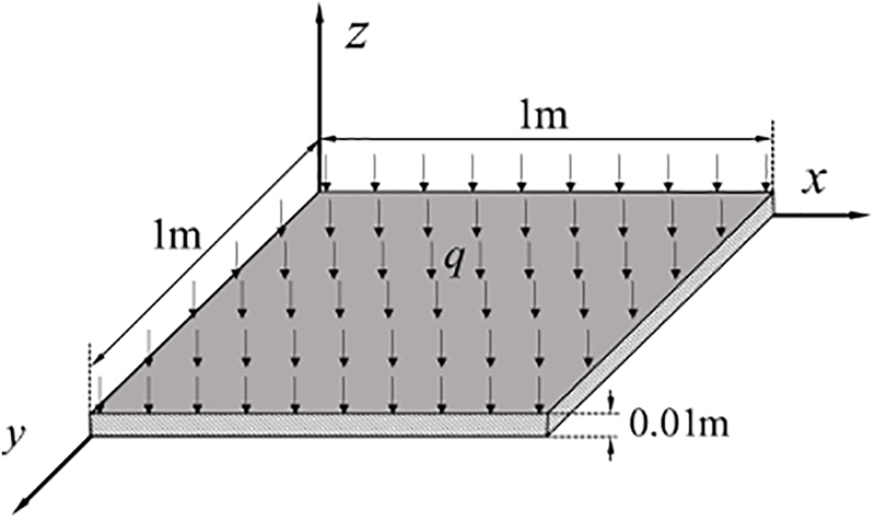
Figure 1: Bending problem of a square thin plate

3.1.1 Standardization of Governing Equations and Boundary Conditions

Under the Kirchhoff hypothesis, the PDE governing the deflection w (x, y) of thin plate bending is [35]

∇2∇2w (x, y)=q/D(6)

where ∇2=∂2/∂x2+∂2/∂y2 is the Laplacian operator; D=Eh3/12(1−ν2) is the flexural rigidity; q=−7×103 Pa is the downward distributed load on the plate. As described in Section 2.1, transitional arguments w1 and w2 are introduced to reduce the fourth-order Eq. (6) as follows:

{∇2(w1+w2)=q/D∂2∂x2w(x, y)=w1∂2∂y2w(x, y)=w2(7)

Hence, the argument u=(w, w1, w2) is composed of three components for this problem.

Thus, the second-order Eq. (7) can be re-arranged as follows:

∇⋅[c1∇Tg1c2∇Tg2c3∇Tg3]uT=ua+f(8)

where c1, c2, c3 and a are matrices; g1, g2, g3 and f are row vectors.

It follows from Eq. (7) that:

{c1=[1001]c2=[1000]c3=[0001]g1=(011)g2=(100)g3=(100)a=[000010001]f=(q/D00)(9)

Correspondingly, the terms Γ and F in the standard form Eq. (2) are

Γ=[c1∇Tg1c2∇Tg2c3∇Tg3]uT=(∂w1∂x+∂w2∂x∂w∂x0∂w1∂y+∂w2∂y0∂w∂y)(10)

and

F=ua+f=(qDw1w2)(11)

Eq. (10) indicates that both Γ and F can be articulated in terms of each component of u. In addition, for this static problem, the mass coefficient ea and the damping coefficient da will vanish in Eq. (2).

The simply supported boundary conditions on the four sides yield

{w(0, y)=0, w1(0, y)=0;w(1, y)=0, w1(1, y)=0w(x, 0)=0, w2(x, 0)=0;w(x, 1)=0, w2(x, 1)=0(12)

Thus, the terms Ri in Eq. (4) are

{R1=(ww10) onx=0R2=(ww10) onx=1R3=(ww20) ony=0R4=(ww20) ony=1(13)

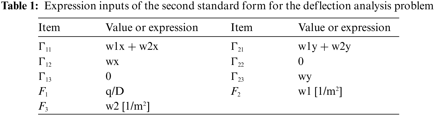
3.1.2 Establishing the Expression Input

After Eqs. (8) and (10) are obtained, it is imperative to establish the corresponding expressions for setting the PDE module.

First, the global parameters are set. Then, the International System of Units (SI) is chosen, and Young’s modulus “E” is 2E11Pa, the Poisson’s ratio “nu” is 0.3, the thickness of plate “h1” is 0.01 m, “q” is −7E3Pa, and the flexural rigidity “D” in Eq. (6) is accordingly calculated.

Next, the equation parameters are set. Based on Eqs. (8) and (2), the number of components of argument u is set to 3, signifying “w” (w), “w1” (w1), and “w2” (w2) in meter. The expression inputs in COMSOL are related to Eqs. (10) and (11) are listed in Table 1. In this table, “wx”, “w1x”, “w2x”, “wy”, “w1y”, and “w2y” represent the partial derivatives for x and y according to the grammar rules in COMSOL, and “[1/m2]” is the dimensional adjustment to guarantee the actual unit 1/m of the components “w1” and “w2” in the row vector u.

3.1.3 Meshing the Plate and Choosing the Shape Functions

This study uses the quadtree refinement technique to mesh the square plate to examine the impact of mesh size on the solution accuracy. For the discretization setting in COMSOL, the free quadrilateral mesh option is first added to generate quadrilateral meshes, and the maximum and minimum sizes are then set to the same h in the mesh size option to obtain a uniform mesh. Fig. 2 shows the generated meshes with h decreases consecutively from 0.1 (a) to 0.05 (b), 0.025 (c), and 0.0125 (d).

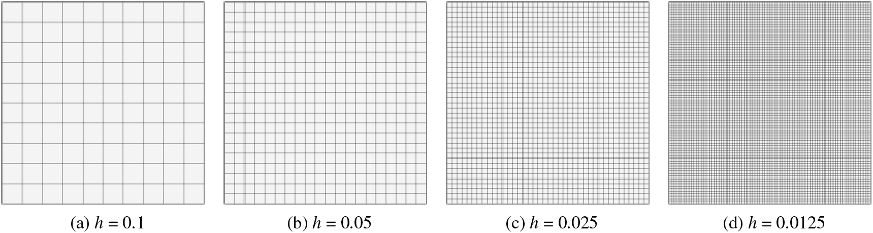
Figure 2: The meshes for the bending problem of square thin plate

In addition, to determine the impact of shape functions on the resolution of the PDE module, the linear shape functions (LSF) and the quadratic shape functions (QSF) are adopted for the four different meshes when setting the chosen physics.

3.2 Stress Analysis of Pure Bending Beam

3.2.1 Standardization of Governing Equations and Boundary Conditions

This section investigates the stress of a pure bending beam. Fig. 3 indicates that the beam is three-dimensional, with a length of 0.1 m and a square cross-section of 0.01 × 0.01 m. The two ends are subjected to a linearly distributed load px varying with the thickness coordinate z, equivalent to the pure bending moment at the two ends. The material is the same as the plate in Fig. 1.

Figure 3: Model of the stress problem of pure bending beam

The equilibrium equations for this problem are [36]

σij,j+fi=0(14)

where σij and fi are the stress tensor and the body force vector, respectively; the indices in Latin letters like i and j range from 1 to 3 with the summation convention for the repeated ones.

For an isotropic material, the constitutive relation is

εij=(1+ν)Eσij−νΘEδij(15)

where Θ=σkk is the trace of stress tensor; εij is the strain tensor.

In addition, the strain tensor accommodates the following compatibility equations:

εij,kl+εkl,ij−εik,jl−εjl,ik=0(16)

Eqs. (14)–(16) are the PDEs for the stress analysis of a pure bending beam. Upon substituting Eq. (15), in terms of stresses, Eq. (16) is reformulated as follows:

(σij,kl+σkl,ij−σik,jl−σjl,ik)=ν(1+ν)(δijΘ,kl+δklΘ,ij−δikΘ,jl−δjlΘ,ik)(17)

By setting l=k, it follows from Eq. (17) that

σij,kk+1(1+ν)Θ,ij−σik,jk−σjk,ik=ν(1+ν)δijΘ,kk(18)

On the other hand, Eq. (14) yields

σik,jk=(σik,k),j=−fi,j(19)

Upon substituting Eqs. (19) and (18) is further expressed as follows:

∇⋅∇Tσij+1(1+v)θ,ij=−v(1−v)δijfk,k−(fi,j+fj,i)(20)

If the case of free body force (fi=0) is considered, Eq. (20) becomes

∇⋅∇Tσij+kΘ,ij=0(21)

where k=1/(1+v).

If σij is denoted by u=(σ11, σ22, σ33, σ12,σ23, σ31), Eq. (21) becomes

∇⋅∇Tu+∇⋅[c1∇Tc2∇Tc3∇Tc4∇Tc5∇Tc6∇T]⋅(c0uT)=0(22)

where the matrices ci(i=1∼6) are

{c1=[100000000]c2=[000010000]c3=[000000001]c4=[010000000]c5=[000001000]c6=[000000100](23)

and the row vector c0 is

c0=(kkk000)(24)

Eq. (22) is not consistent with the first standard form Eq. (1). In contrast, the terms in the second standard form Eq. (2) are

Γ=∇Tu+[c1∇Tc2∇Tc3∇Tc4∇Tc5∇Tc6∇T](c0uT)=(∂σ11∂x+k∂Θ∂x∂σ22∂x∂σ33∂x∂σ12∂x+k∂Θ∂y∂σ23∂x∂σ31∂x∂σ11∂y∂σ22∂y+k∂Θ∂y∂σ33∂y∂σ12∂y∂σ23∂y+k∂Θ∂z∂σ31∂y∂σ11∂z∂σ22∂z∂σ33∂z+k∂Θ∂z∂σ12∂z∂σ23∂z∂σ31∂z+k∂Θ∂x)(25)

and

F=(000000)(26)

On the other hand, this study introduces the following notions:

{∇1}={∂/∂x, ∂/∂y,  ∂/∂z, ∂/∂x, ∂/∂y, ∂/∂z}T{∇2}={∂/∂x, ∂/∂y, ∂/∂z,∂/∂y, ∂/∂z, ∂/∂x}T(27)

and σ=(σ11, σ22, σ33, σ12, σ23, σ31).

Eq. (22) is thus re-expressed as follows:

∇2σ+k{∇1}⊙{∇2}Θ=0(28)

where ⊙ is the Hadamard product operator.

From the calculus of variation, it follows from Eq. (28) that

∫Ωσ∼T(∇2σ+k{∇1}⊙{∇2}Θ)dV=0(29)

where σ∼ is the row form of trial functions corresponding to σ.

Integration by parts, Eq. (29) yields.

∫Ω[−σ∼,iTσ,i−k({∇1}T⊙σ∼T{∇2}Θ)]dV+∫∂Ω[(σ∼Tσ,i)ni+k(σ∼T⊙{∇1}TΘ){n1}]dS=0(30)

where ni=nx, ny or nz and {n1}={nx, ny, nz, nx, ny, nz}T.

The terms in the third standard form Eq. (3) are

weaks=−σ∼,iTσ,i−k[{∇k}T⊙σ∼T{∇l}Θ]=∑j=16weakj(31)

and

weakb=(σ∼Tσ,i)ni+k(σ∼T⊙{∇l}TΘ){nk}(32)

where

{weak1=−(σ∼11,1σ11,1+σ∼11,2σ11,2+σ∼11,3σ11,3)−k[σ∼11,1(σ11,1+σ22,1+σ33,1)]weak2=−(σ∼22,1σ22,1+σ∼22,2σ22,2+σ~22,3σ22,3)−k[σ∼22,2(σ11,2+σ22,2+σ33,2)]weak3=−(σ∼33,1σ33,1+σ∼33,2σ33,2+σ∼33,3σ33,3)−k[σ∼33,3(σ11,3+σ22,3+σ33,3)]weak4=−(σ∼12,1σ12,1+σ∼12,2σ12,2+σ∼12,3σ12,3)−k[σ∼12,1(σ11,2+σ22,2+σ33,2)]weak5=−(σ∼23,1σ23,1+σ∼23,2σ23,2+σ∼23,3σ23,3)−k[σ∼23,2(σ11,3+σ22,3+σ33,3)]weak6=−(σ∼31,1σ31,1+σ∼31,2σ31,2+σ∼31,3σ31,3)−k[σ∼31,3(σ11,1+σ22,1+σ33,1)](33)

Next, the prescription of boundary conditions is discussed.

This study emphasizes that the weak form weakb in Eq. (32) vanishes on the boundary ∂Ω in the proposed case because the boundary conditions will be directly prescribed for the relevant boundaries.

The following boundary conditions are described on the six faces of this beam structure:

{σ11(x, y, z)=pxon x=0or0.1σij(x, y, z)=0 elsewhere(34)

where px=p0(z−h1/2) with h1=0.01 m and p0=105 Pa.

Eq. (21) is indeterminate because the six equations are not independent. Hence, as the supplementary constraints, Eq. (14) must be adopted. However, if the constraints are applied pointwise in the domain Ω, the cost must significantly increase to reduce the solution efficiency. In virtue of this, considering the harmonic nature of σij,j+fi (see Eq. (19)), the pointwise constraints (14) in the domain Ω are replaced by the pointwise constraints (5) on boundary ∂Ω [36] as

Pi=σij,j+fi(35)

3.2.2 Establishing the Expression Input

Following the same steps in Section 3.1.2, this study sets the global parameters such as “E”, “nu” and “p0” = 1E5 Pa.

Based on Eq. (22), the argument u has six components, (s11, s22, s33, s12, s23, and s31), representing six components (σ11, σ22, σ33, σ12,σ23, σ31) of the stress tensor, respectively.

For the second standard form, the conservation flux Γ is a 3 × 6 matrix as Eq. (25), and the source term F is a 1 × 6 row vector as Eq. (26). The expression inputs to COMSOL are listed in Table 2. Each expression follows the grammar rules in COMSOL. In addition, to simplify Γ, Θ is denoted by the symbol “h” and “d(h, x)”, for example, signifies the partial derivative of “h” with respect to coordinate x.

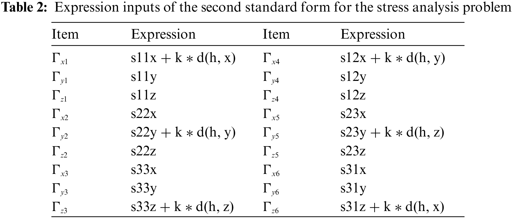
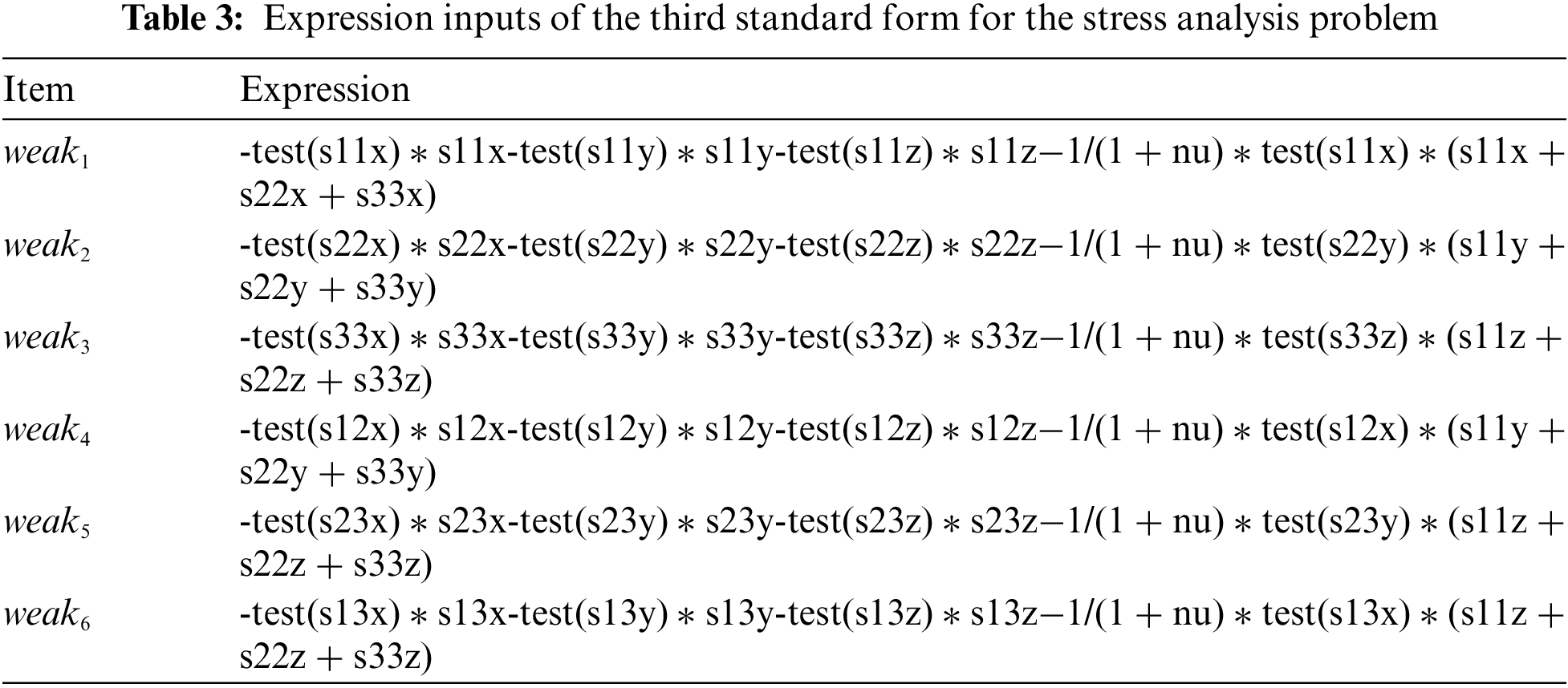
Similarly, it can obtain the expression inputs based on Eqs. (31) and (33) for the third standard form, which is summarized in Table 3 with test (s11x), for example, signifying the derivative of s11 test function with respect to x based on the grammar rules in COMSOL.

Based on Eq. (4), boundary conditions (34) are prescribed through the following settings:

1) Select the two faces of x=0 and x=0.1, and set the boundary constraints as

   R1=(s11−p0*(z−h1/2)s12s31000)(36)

2) Select the two faces of y=0 and y=0.1, and set the boundary constraints as

   R2=(s12s22s23000)(37)

3) Select the two faces of z=0 and z=0.01, and set the boundary constraints as

   R3=(s31s23s33000)(38)

Based on Eq. (5), pointwise constraints (35) are prescribed on the six faces of beam through the settings as

{P1=s11x+s12y+s31zP2=s12x+s22y+s23zP3=s31x+s23y+s33z(39)

3.2.3 Meshing the Beam and Choosing the Shape Functions

For this three-dimensional problem, four meshes with consecutively decreasing size are examined. In COMSOL, a three-dimensional mesh is accomplished through a sweeping technique. Hence, the free quadrilateral mesh option is first added on x=0 as the boundary selection for the option over which a uniform mesh is generated by setting the mesh size h. The swept option is then added on x=0 as the source face and on x=0.1 as the destination face by setting the same h. Fig. 4 depicts the generated meshes. When h decreases consecutively from 0.01 (a) to 0.005 (b), 0.0025 (c), and 0.00125 (d).

Figure 4: The meshes for the pure bending beam problem

The setting of shape functions is the same as in Section 3.1.3.

4  Results and Discussion

4.1 Results for the Deflection of thin Plate Bending

For this thin plate bending problem, this study can get the Levy series solution [36] as the reference.

Section 3.1 completed the PDE module settings for the solution to the deflection of thin plate bending. The argument u can be obtained for this problem using the default settings of the stationary solver. The results are shown in Fig. 5. The QSF and the LSF can give satisfactory deflection for the four meshes.

Figure 5: Results comparison of the deflection of thin plate bending

In order to show the mesh-dependent convergence, this study examines the L2-error norm (RE) in deflection as

RE=∑i=1N(wPDEi−wRefi)2/∑i=1N(wRefi)2(40)

where N is the total number of nodes in the mesh; wPDEi and wRefi are the results from the PDE module and the reference solution.

The RE is depicted in Fig. 6, where L is the length of the square thin plate. The error norms decrease monotonically for both the QSF and the LSF as the mesh size h reduces.

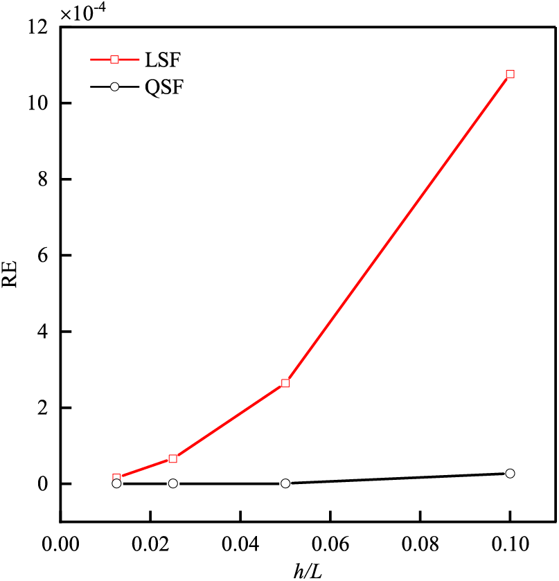
Figure 6: Variation of RE with the mesh size for the deflection of thin plate bending

4.2 Results for the Stress of the Pure Bending Beam

For a pure bending problem, from the fundamental mechanics of materials, the reference solution for the normal stress σ11 in the cross-section is linear along the thickness as

σ11=z/h1 ∗ 500(MPa)(41)

Section 3.2 completed the PDE settings for this problem for the second standard form as Eqs. (25) and (26), and the third standard form as Eq. (30).

Fig. 7 illustrates the results obtained using the default stationary solver. It indicates that the distribution and the magnitude are correct only for the LSF. Variation of the RE in stress σ11 is depicted in Fig. 8 as compared to the reference, where L is the length of the beam. The results converge with the reference for the LSF but not the QSF.

Figure 7: Results comparison of the pure bending problem

Figure 8: Variation of RE with the mesh size for the stress of pure bending beam

If the results from the PDE module are used under the finest mesh in Fig. 4d at h = 0.00125 as the new reference and re-evaluate the RE in stress σ11 for the QSF, the blue plot (marked by QSF-R) is obtained as shown in Fig. 8. This indicates that the results converge per se as the mesh size decreases when using the QSF, which differs from the solution of a pure bending beam. This is due to the inappropriate prescription of the pointwise constraints Eq. (39) when the arguments (stresses in the proposed case) within each element are interpolated with the QSF.

5  Conclusion

This study investigates the three standard forms of PDE module in COMSOL and their application to two mechanics problems. The results agree very well with the literature. The current research indicated that the PDE module can be employed to address problems to which the FEM is not applicable as long as the problem is transferred to one of the three standard forms.

In the stress analysis of a pure bending beam, the second-order compatibility equations are the governing equations, while the first-order equilibrium equations are the supplementary constraints. In addition, the current practice indicates that care must be considered for the shape functions when supplementary constraints are enforced on the boundary.

The limitation of this paper lies in that, while extending the applicable scope, the threshold is elevated for the user of the PDE module, and expertise in various aspects is hence required, such as formulation skills, knowledge of calculus of variations, and assessment of results in convergence and accuracy.

Acknowledgement: The authors express gratitude to the editors and reviewers for their valuable suggestions on this paper.

Funding Statement: This work was partly supported by the National Natural Science Foundations of China (Grant Nos. 12372073 and U20B2013) and the Natural Science Basic Research Program of Shaanxi (Program No. 2023-JC-QN-0030).

Author Contributions: The authors confirm their contribution to the paper as follows: study conception and design: Ningjie Wang, Luxian Li; data collection: Ningjie Wang, Yihao Wang, Yongle Pei; analysis and interpretation of results: Ningjie Wang, Yihao Wang, Luxian Li; draft manuscript preparation: Ningjie Wang, Luxian Li. All authors reviewed the results and approved the final version of the manuscript.

Availability of Data and Materials: The data will be made available by the corresponding author upon reasonable request.

Ethics Approval: Not applicable.

Conflicts of Interest: The authors declare that they have no conflicts of interest to report regarding the present study.

References

1. Lu P, He LH, Lee HP, Lu C. Thin plate theory including surface effects. Int J Solids Struct. 2006;43:4631–47. doi:10.1016/j.ijsolstr.2005.07.036. [Google Scholar] [CrossRef]

2. Ahmed AM, Rifai AM. Euler-bernoulli and timoshenko beam theories analytical and numerical comprehensive revision. Eur J Eng Tech Res. 2021;6:20–32. doi:10.24018/ejeng.2021.6.7.2626. [Google Scholar] [CrossRef]

3. Vajjala KS, Sengupta TK, Mathur JS. Effects of numerical anti-diffusion in closed unsteady flows governed by two-dimensional Navier-Stokes equation. Comput Fluids. 2020;201:104479. doi:10.1016/j.compfluid.2020.104479. [Google Scholar] [CrossRef]

4. Fu Z, Xu W, Liu S. Physics-informed kernel function neural networks for solving partial differential equations. Neural Netw. 2024;172:106098. doi:10.1016/j.neunet.2024.106098. [Google Scholar] [PubMed] [CrossRef]

5. Van Vinh P, Van Chinh N, Tounsi A. Static bending and buckling analysis of bi-directional functionally graded porous plates using an improved first-order shear deformation theory and FEM. Eur J Mech A-Solid. 2022;96:104743. doi:10.1016/j.euromechsol.2022.104743. [Google Scholar] [CrossRef]

6. Oukaira A, Said D, Mellal I, Ettahri O, Zbitou J, Lakhssassi A. Thermal camera for system-in-package (SiP) technology: transient thermal analysis based on FPGA and finite element method (FEM). AEU-Int J Electron C. 2023;172:154980. doi:10.1016/j.aeue.2023.154980. [Google Scholar] [CrossRef]

7. Zhang RL, Wu CJ, Zhang YT. A novel technique to predict harmonic response of particle-damping structure based on ANSYS® secondary development technology. Int J Mech Sci. 2018;144:877–86. doi:10.1016/j.ijmecsci.2017.10.035. [Google Scholar] [CrossRef]

8. Nguyen-Xuan H, Chau KN, Chau KN. Polytopal composite finite elements. Comput Methods Appl Mech Eng. 2019;355:405–37. doi:10.1016/j.cma.2019.06. [Google Scholar] [CrossRef]

9. İynen O, Ekşi AK, Akyıldız HK, Özdemir M. Real 3D turning simulation of materials with cylindrical shapes using ABAQUS/Explicit. J Braz Soc Mech Sci Eng. 2021;43:374. doi:10.1007/s40430-021-03075-5. [Google Scholar] [CrossRef]

10. Swamy Yadav G, Anuradha P. Strain investigation of infill frames using FEA package MSC NASTRAN. Adv Eng Softw. 2021;154:102975. doi:10.1016/j.advengsoft.2021.102975. [Google Scholar] [CrossRef]

11. Sarkar S, Singh IV, Mishra BK. A simple and efficient implementation of localizing gradient damage method in COMSOL for fracture simulation. Eng Fract Mech. 2022;269:108552. doi:10.1016/j.engfracmech.2022.108552. [Google Scholar] [CrossRef]

12. Goodfellow I, Bengio Y, Courville A. Deep learning. Cambridge, MA, USA: MIT Press; 2016. [Google Scholar]

13. He K, Zhang X, Ren S, Sun J. Deep residual learning for image recognition. In: Proceedings of the IEEE Conference on Computer Vision and Pattern Recognition, 2016; Las Vegas, NV, USA. p. 770–8. [Google Scholar]

14. Cuomo S, Di Cola VS, Giampaolo F, Rozza G, Raissi M, Piccialli F. Scientific machine learning through physics-informed neural networks: where we are and what’s next. J Sci Comput. 2022;92:1–62. doi:10.1007/s10915-022-01939-z. [Google Scholar] [CrossRef]

15. Nghia-Nguyen T, Kikumoto M, Nguyen-Xuan H, Khatir S, Abdel Wahab M, Cuong-Le T. Optimization of artificial neutral networks architecture for predicting compression parameters using piezocone penetration test. Expert Syst Appl. 2023;223:119832. doi:10.1016/j.eswa.2023.119832. [Google Scholar] [CrossRef]

16. Liu Z, Yang Y, Cai Q. Neural network as a function approximator and its application in solving differential equations. Appl Math Mech. 2019;40:237–48. doi:10.1007/s10483-019-2429-8. [Google Scholar] [CrossRef]

17. Sirignano J, Spiliopoulos K. DGM: a deep learning algorithm for solving partial differential equations. J Comput Phys. 2018;375:1339–64. doi:10.48550/arXiv.2010.08895. [Google Scholar] [CrossRef]

18. Raissi M, Perdikaris P, Karniadakis GE. Physics-informed neural networks: a deep learning framework for solving forward and inverse problems involving nonlinear partial differential equations. J Comput Phys. 2019;378:686–707. doi:10.48550/arXiv.230608827. [Google Scholar] [CrossRef]

19. Zha W, Li D, Shen L, Zhang W, Liu X. Review of neural network-based methods for solving partial differential equations. Chi J Thero App Mech. 2022;54:543–56. doi:10.6052/0459-1879-21-617. [Google Scholar] [CrossRef]

20. Gao P, Zhao Z, Yang Y. Study on numerical solutions to hyperbolic partial differential equations based on the convolutional neural network model. Appl Math Mech. 2021;42:932–47. doi:10.21656/1000-0887.420050. [Google Scholar] [CrossRef]

21. Li Z, Kovachki N, Azizzadenesheli K, Liu B, Bhattacharya K, Stuart A, et al. Fourier neural operator for parametric partial differential equations; 2020. doi:10.48550/arXiv.2010.08895. [Google Scholar] [CrossRef]

22. Hao Z, Yao J, Su C, Su H, Wang Z, Lu F, et al. Pinnacle: a comprehensive benchmark of physics-informed neural networks for solving pdes; 2023. doi:10.48550/arXiv.230608827. [Google Scholar] [CrossRef]

23. Haghighat E, Raissi M, Moure A, Gomez H, Juanes R. A physics-informed deep learning framework for inversion and surrogate modeling in solid mechanics. Comput Methods Appl Mech Eng. 2021;379:113741. doi:10.1016/j.cma.2021.113741. [Google Scholar] [CrossRef]

24. Kochkov D, Smith JA, Alieva A, Wang Q, Brenner MP, Hoyer S. Machine learning-accelerated computational fluid dynamics. Proc Natl Acad Sci. 2021;118:e2101784118. doi:10.1073/pnas.2101784118. [Google Scholar] [PubMed] [CrossRef]

25. Azizzadenesheli K, Kovachki N, Li Z, Liu-Schiaffini M, Kossaifi J, Anandkumar A. Neural operators for accelerating scientific simulations and design. Nat Rev Phys. 2024;6:320–8. doi:10.1038/s42254-024-00712-5. [Google Scholar] [CrossRef]

26. Lorenzen F, Zargaran A, Janoske U. Potential of physics-informed neural networks for solving fluid flow problems with parametric boundary conditions. Phys Fluids. 2024;36:037143. doi:10.1063/5.0193952. [Google Scholar] [CrossRef]

27. Yang F, Liang QC, Qiao RP, He JN. Modeling and simulation of ammonia hydrogen reactor based on COMSOL. J Phys Conf Ser. 2021;1948:012197. doi:10.1088/1742-6596/1948/1/012197. [Google Scholar] [CrossRef]

28. Badawi MB, Crosby WA, El Fahham IM, Alkomy MH. Performance analysis of tilting pad journal bearing using COMSOL Multiphysics and Neural Networks. Alexandria Eng J. 2020;59:865–81. doi:10.1016/j.aej.2020.03.015. [Google Scholar] [CrossRef]

29. Wijayanti W, Sasongko MN, Kusumastuti R. Modelling analysis of pyrolysis process with thermal effects by using comsol multiphysics. Case Stud Therm Eng. 2021;28:101625. doi:10.1016/j.csite.2021.101625. [Google Scholar] [CrossRef]

30. Wang Y, Chen J, Li D, Shi L, Chi H, Ma Y. Simulation of SN transport equation for hexagonal-z reactor using the COMSOL Multiphysics software. Nucl Eng Des. 2024;416:112746. doi:10.1016/j.nucengdes.2023.112746. [Google Scholar] [CrossRef]

31. Yılmaz F, Karasözen B. Solving optimal control problems for the unsteady burgers equation in COMSOL multiphysics. J Comput Appl Math. 2011;235:4839–50. doi:10.1016/j.cam.2011.01.002. [Google Scholar] [CrossRef]

32. Zhou J, Wei C, Li W, Chen H. Analysis of solid elastoplastic mechanics based on mathematical module of COMSOL Multiphysics. Eng J Wuhan Univ. 2015;48:195–201. doi:10.14188/i.1671-8844.2015-02-011. [Google Scholar] [CrossRef]

33. Wu D. Variational method. Beijing, China: Higher Education Press; 1987 (In Chinese). [Google Scholar]

34. Roul P, Goura VP, Agarwal R. A compact finite difference method for a general class of nonlinear singular boundary value problems with Neumann and Robin boundary conditions. Appl Math Comput. 2019;350:283–304. doi:10.1016/j.amc.2019.01.001. [Google Scholar] [CrossRef]

35. Stempin P, Pawlak TP, Sumelka W. Formulation of non-local space-fractional plate model and validation for composite micro-plates. Int J Eng Sci. 2023;192:103932. doi:10.1016/j.ijengsci.2023.103932. [Google Scholar] [CrossRef]

36. Lu M, Luo X. Foundations of elasticity. Beijing, China: Tsinghua University Press; 1990 (In Chinese). [Google Scholar]