Analysis of Progressively Type-II Inverted Generalized Gamma Censored Data and Its Engineering Application

1  Introduction

Recently, we have come across several studies on inverse (or reciprocal) distributions of one or two parameters in the literature. Louzada et al. [1] recently emphasized that inverse distributions provide greater flexibility for fitting data and, in many cases, have been found to be better than many other standard distributions. The three parameter inverted generalized gamma (IGG) distribution was introduced by Hoq et al. [2] in the context of life testing experiments. As specific examples, the IGG distribution includes a number of lifespan distributions, including inverted gamma, inverted half-normal, inverted Weibull, inverted exponential, inverted Rayleigh, inverted Maxwell-Boltzmann, and inverted chi-square. The IGG distribution has been found to be a good alternative to other skewed distributions, including inverse gamma, inverse Weibull, and generalized inverse exponential distributions, and can be used to illustrate skewed data.

A random variable x is said to have IGG (Υ) distribution, where Υ=(δ,μ,σ)⊤, if its cumulative distribution function (CDF) and probability density function (PDF) are given, respectively, by

F(x;Υ)=1−1Γ(μ)γ(μ,σδx−δ), x>0,(1)

and

f(x;Υ)=δΓ(μ)σδμx−δμ−1e−σδx−δ,(2)

where (δ,μ)>0 (denote the shape parameters) and σ>0 (denotes the scale parameter). The reliability function (say, R(t)) and hazard rate function (say, h(t)) are, respectively, given by

R(t;Υ)=1Γ(μ)γ(μ,σδt−δ), t>0,(3)

and

h(t;Υ)=δσδμγ(μ,σδt−δ)t−δμ−1e−σδt−δ, t>0,(4)

where γ(a,b)=∫0bua−1e−udu and Γ(ξ)=∫0∞tξ−1e−tdt.

The hazard rate function (4) has an unimodal shape, while the density function (2) is unimodal and right-skewed with heavy tails. These tails become thicker when the shape parameters are equal, and longer when the shape parameter δ increases.

Besides Type-I, Type-II, and progressive Type-II censoring (PT2C) plans, several censoring mechanisms are available in the literature. An important advantage of PT2C is that it allows the experimenter to withdraw some live units before the experiment stops. The PT2C can be described as follows: Suppose we have n identical and independent units. The effective size (say, m) and the progressive censoring (say, R=(R1,R2,⋯,Rm)) must be determined in advance. When the first failure occurs (say, X1:m:n), R1 (from n−1) of live units are randomly selected and excluded from the test. Likewise, in case of the second failure X2:m:n, we randomly remove R2 from n−R1−2 live units. Once the mth failure is recorded, all remaining surviving items Rm=n−m−∑i=1m−1Ri are eliminated. For more details; see Balakrishnan et al. [3].

The maximum product spacing (MPS) was initially presented by Cheng et al. [4] and was utilized by Ranneby [5] as an alternative to the maximum likelihood (ML) estimation approach. In recent times, the MPS method has been employed in different contexts; see Zhu [6], Jeon et al. [7], Nassar et al. [8], Nassar et al. [9], and many others. According to Anatolyev et al. [10], the MPS approach adheres to the invariance property and outperforms likelihood estimators in small-sample scenarios for heavy and skewed distributions.

The limitations and challenges of this work are particularly related to the complexity of parameter estimation, computational intensity, small sample sizes, model power, hypothesis testing, and inference difficulties. Addressing these issues often requires advanced statistical techniques and careful consideration of the specific characteristics of the data and the censoring scheme.

Researchers pay little attention to analyzing new extended gamma lifetime models because of their complex results and expensive numerical evaluations. Aside from the work of Ramos et al. [11], as they studied Bayesian inferences based on non-informative priors using a complete sample, and no attempt has been made, to our knowledge, to estimate IGG parameters based on PT2C since the IGG distribution was introduced in the literature.

Given the usefulness and practicality of the IGG distribution, and with samples collected from the PT2C strategy, we state our main objectives in this paper as follows:

•   Obtain the frequentist point estimators of the parameters (including Υ, R(t), and h(t)) through the ML and MPS methods of estimation.

•   Obtain the approximate confidence intervals (ACIs) for all parameters using the acquired ML estimators (MLEs) and MPS estimators (MPSEs).

•   As an alternative to the ML function in the Bayesian paradigm, the MPS function is also taken into consideration. Next, both ML and MPS functions are explored in a Bayesian framework for all unknown parameters under squared error loss (SEL) with independent gamma priors.

•   Implement Markov chain Monte Carlo (MCMC) methodology with Metropolis–Hastings (M–H) sampler to calculate the offered Bayes point estimates as well as Bayes confidence intervals (BCIs).

•   Various optimality metrics are assessed to provide the optimal PT2C plan.

•   Extensive Monte Carlo simulations are performed to evaluate the performance of the proposed techniques.

•   An engineering data set representing diesel engine failure times is analyzed to show the applicability of the proposed methodologies in a real-life scenario.

The rest of the article is organized as follows: In Sections 2 and 3, we discuss ML- and MPS-based estimation. In Section 4, we discuss Bayesian inferences. Simulation investigations are highlighted in Section 5. In Section 6, the optimal PT2C is discussed. One real data set is analyzed in Section 7. Finally, various observations are made in Section 8.

2  Likelihood Estimation

This section considers the ML estimation to provide the MLEs along with their ACIs of the IGG parameters δ, μ, σ, R(t), and h(t) using the PT2C sample.

2.1 The MLEs

Suppose x=(xi,Ri), i=1,2,…,m, where xi is used in place of xi:m:n, is an observed PT2C sample obtained from the IGG (Υ) distribution. From (2) and (1), the likelihood function (LF) becomes

L(δ,μ,σ|x) =A∏i=1mf(xi;δ,μ,σ)[1−F(xi;δ,μ,σ)]Ri, =A(δΓ(μ))mσmδμ∏i=1mxi−δμ−1e−σδxi−δ[1Γ(μ)γ(μ,σδxi−δ)]Ri,(5)

where A=n(n−R1−1)⋯(n−(m−1)−∑i=1m−1Ri).

Using (5), without constant terms, the log-likelihood function ℓ∝L(⋅) can be written as

ℓ∝mln⁡(δ)−nln⁡(Γ(μ))+mδμln⁡(σ)−(δμ+1)∑i=1mln⁡(xi)−∑i=1m(σxi−1)δ+∑i=1mRiln⁡(ψi),(6)

where ψi=γ(μ,(σ/xi )δ).

The MLEs δ^, μ^, and σ^ of δ, μ, and σ, can be offered by differentiating (6) with respect to δ, μ, and σ, respectively, as

∂ℓ∂δ=mδ+μ(mln⁡(σ)−∑i=1mln⁡(xi))−∑i=1m(σxi−1)δln⁡(σxi−1)+∑i=1mRiψi(δ′),(7)

∂ℓ∂μ=−nη(μ)+δ(mln⁡(σ)−∑i=1mln⁡(xi))+∑i=1mRiψi(μ′),(8)

and

∂ℓ∂σ=δσ[mμ−∑i=1m(σxi−1)δ]+∑i=1mRiψi(σ′),(9)

where η(μ)=dln⁡(Γ(μ))/dμ is the digamma function and ψi(ξ′) is the first-partial derivative with respect to ξ as

ψi(δ′)=∂∂δln⁡(γ(μ,(σxi−1 )δ))=ψi−1(σxi−1)δμln⁡(σxi−1)exp⁡(−(σxi−1)δ)

ψi(μ′)=∂∂μln⁡(γ(μ,(σxi−1 )δ))=ψi−1∫0(σxi−1)δwμ−1ln⁡(w)e−wdw,

and

ψi(σ′)=∂∂σln⁡(γ(μ,(σxi−1)δ))=ψi−1δσ(σxi−1)δμexp⁡(−(σxi−1)δ).

To prove the convergence of the MLEs δ^, μ^, and σ^ of δ, μ, and σ, respectively, the offered form in (6) makes it difficult to verify these features theoretically. To solve this problem, we simulate a PT2C sample from IGG (1,1.5,0.5) when (n,m)=(50,25) and Ri=1, i=1,…,m. As a result, we find that (δ^,μ^,σ^) = (1.1621,1.4558,0.6533). In Fig. 1, the log-LF line and its normal-equation curve of δ^, μ^, and σ^ are depicted. To distinguish, for each sup-plot in Fig. 1, we plot the log-LF curve (in red at the apex) and the first-partial derivative (FPD) curve (in black at the zero point) intersect at the vertical line (which represents the MLE of δ, μ, or σ). Since we obtained the estimated values of the MLEs, this indicates that the proposed likelihood equations converge well. At the same time, the MLEs δ^, μ^, and σ^ exist and are unique. The invariance feature of δ^, μ^, and σ^ makes it easy to acquire the MLEs of R(t) (3) and h(t) (4) at time t>0 once the MLEs of δ, μ, and σ have been obtained.

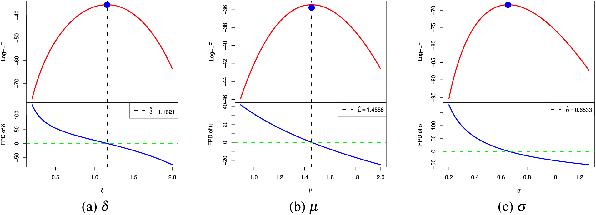
Figure 1: The log-LF (top) and its FPD (bottom) of (a) δ, (b) μ, and (c) σ

2.2 ACIs via LF-Based

In this subsection, the (1−ρ)% ACIs of δ, μ, σ, R(t), and h(t) are obtained. First, from (6), the second derivatives with respect to δ, μ, and σ are obtained and reported in Appendix A. It is clear that the issue of obtaining asymptomatic expressions for the variances and covariances of δ^, μ^, and σ^ is tedious. We thus estimate the variance-covariance (V-C) matrix (say, I1−1(⋅)), where I1(⋅) is the observed Fisher’s information, using the LF-based as

I1−1(δ^,μ^,σ^)=[−ℓ11−ℓ12−ℓ13−ℓ22−ℓ23−ℓ33](δ^,μ^,σ^)−1=[var^(δ^)cov^(δ^,μ^)cov^(δ^,σ^)var^(μ^)cov^(μ^,σ^)var^(σ^)].(10)

It is established that (δ^,μ^,σ^)∼N((δ,μ,σ),I1−1(δ^,μ^,σ^)). Consequently, the (1−ρ)% ACIs of δ, μ, and σ are given, respectively, by

δ^±zρ/2var^(δ^),μ^±zρ/2var^(μ^),andσ^±zρ/2var^(σ^),

where zρ/2 is the upper (ρ/2)th standard-normal percentile point.

To find the (1−ρ)% ACIs of R(t) and h(t), we use the delta method; see Greene [12]. Next, the approximated variances of R^(t) and h^(t) (after getting (δ^,μ^,σ^)) can be obtained as

var^(R^(t))=[∇R(t)]TI1−1(δ,μ,σ)[∇R(t)]|(δ^,μ^,σ^) and var^(h^(t))=[∇h(t)]TI1−1(δ,μ,σ)[∇h(t)]|(δ^,μ^,σ^),

where ∇R^(t) and ∇h^(t) are the estimated gradient of R(t) and h(t), respectively.

Hence, once we obtain the variances var^(R^(t)) and var^(h^(t)), then 100(1−ρ)% two-sided ACIs for R(t) and h(t) are given by

R^(t)±zρ/2var^(R^(t))andh^(t)±zρ/2var^(h^(t)),

respectively, where zρ/2 is the right-tail (ρ/2)th standard-normal point.

3  Product of Spacings Estimation

This section examines the MPS estimation approach to acquire the MPSEs and ACIs of δ, μ, σ, R(t), and h(t) based on the PT2C sample.

3.1 The MPSEs

Substituting (2) and (1) into the product of spacing (PS) function of PT2C, we get the joint PS function of δ, μ, and σ as follows:

S(δ,μ,σ) =∏i=1m+1[F(xi;δ,μ,σ)−F(xi−1;δ,μ,σ)]∏i=1m[1−F(xi;δ,μ,σ)]Ri, =∏m+1i=1[1Γ(μ)γ(μ,(σxi−1)δ)−1Γ(μ)γ(μ,(σxi)δ)]∏mi=1[1Γ(μ)γ(μ,(σxi)δ)]Ri,(11)

where F(x0;δ,μ,σ)≡0 and F(xm+1;δ,μ,σ)≡1.

By maximizing the following logarithmic MPS function (e.g., ln⁡S) with respect to δ, μ, and σ, one can obtain their MPSEs as follows:

ln⁡S∝−(n+1)ln⁡Γ(μ)+∑i=1m+1ln⁡(ψi−1−ψi)+∑i=1mRiln⁡ψi,(12)

where ψi−1=γ(μ,(σxi−1−1)δ) and ψi=γ(μ,(σxi−1)δ).

Solving the following three normal equations will yield the MPSEs of δ, μ, and σ, denoted by δ~, μ~, and σ~, respectively:

∂ln⁡S∂δ=∑i=1m+1[ψi−1(δ′)−ψi(δ′)ψi−1−ψi]+∑i=1mRiψi(δ′),(13)

∂ln⁡S∂μ=−(n+1)η(μ)+∑i=1m+1[ψi−1(μ′)−ψi(μ′)ψi−1−ψi]+∑i=1mRiψi(μ′),(14)

and

∂ln⁡S∂σ=∑i=1m+1[ψi−1(σ′)−ψi(σ′)ψi−1−ψi]+∑i=1mRiψi(σ′),(15)

where ψi−1(ξ′) is the first-partial derivative of ψi−1 with respect to ξ.

Since the proposed MPSEs from (13)–(15) lack closed form solutions, an iterative method such as Newton-Raphson can be easily used to derive the MPSEs numerically. It is important to note that the MPSEs and MLEs of δ, μ, and σ have several flexible qualities, such as consistency, asymptotic efficiency, and invariance.

Now, to highlight the convergence of the MPSEs δ~, μ~, and σ~ of δ, μ, and σ, respectively, the offered form in (12) makes it not easy. Using the same PT2C sample generated in Subsection 2.1, we have (δ~,μ~,σ~) = (1.2729,1.4557,0.5154). Fig. 2 supports this result. It indicates that the suggested normal equations used to create the MPSEs converge well. It also indicates that the MPSEs δ~, μ~, and σ~ exist and are unique.

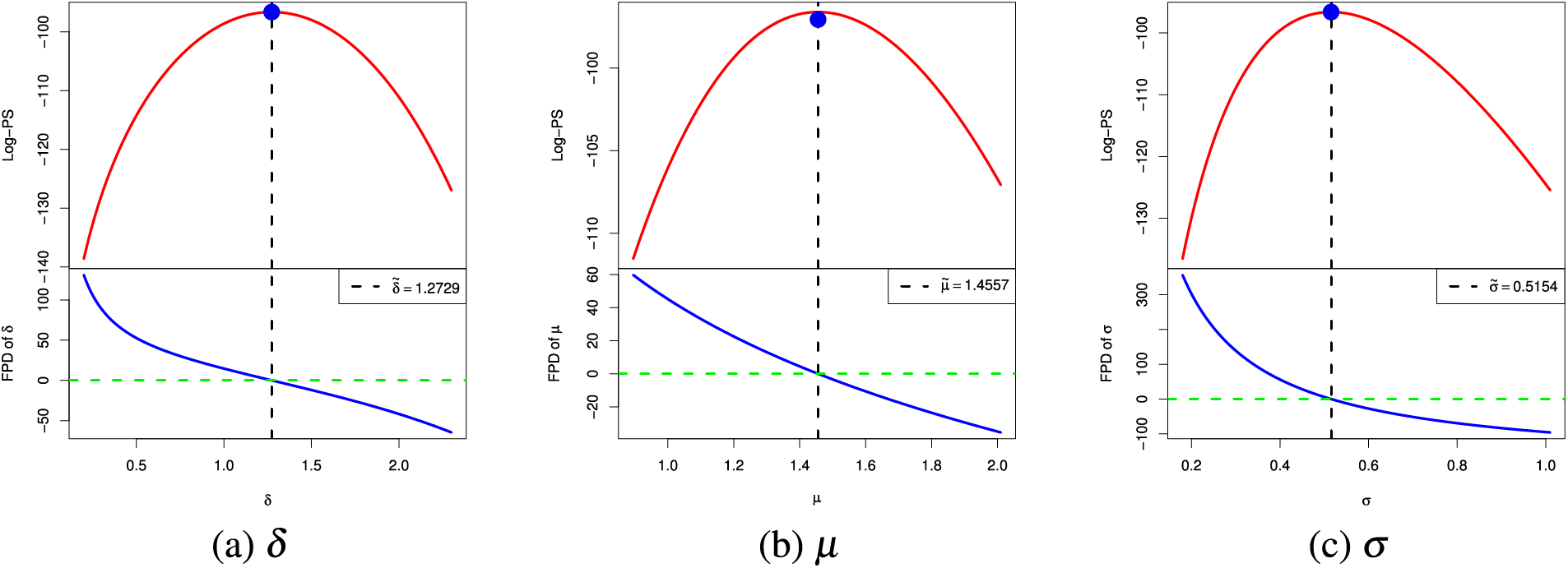
Figure 2: The log-PS (top) and its FPD (bottom) of (a) δ, (b) μ, and (c) σ

3.2 ACIs via PS-Based

To get the two bounds (1−ρ)% ACIs (PS-based) of the δ, μ, σ, R(t), or h(t), the second derivatives of (12) with respect to δ, μ, and σ should be first obtained; see Appendix B. Since the exact expectations of Sij, i,j=1,2,3 cannot be solved analytically, similar to the case of Fisher information using LF-based, the approximated V-C matrix of the MPSEs can be obtained as

I2−1(δ~,μ~,σ~)=[−S11−S12−S13−S22−S23−S33](δ~,μ~,σ~)−1=[var~(δ~)cov~(δ~,μ~)cov~(δ~,σ~)var~(μ~)cov~(μ~,σ~)var~(σ~)].(16)

It follows that (δ~,μ~,σ~)∼N((δ,μ,σ),I2−1(δ~,μ~,σ~)), where I2−1(δ~,μ~,σ~) is given by (16). Consequently, the respective (1−ρ)% ACIs (PS-based) of δ, μ, and σ are

δ~±zρ/2var~(δ~), μ~±zρ/2var~(μ~),andσ~±zρ/2var~(σ~).

Replacing δ, μ, and σ in (3) and (4) by their MPSEs δ~, μ~, and σ~, respectively, the MPSEs R~(t) and h~(t) can be easily derived. Thus, the 100(1−ρ)% ACIs (PS-based) of R(t) and h(t) are given by

R~(t)±zρ/2var~(R~(t))andh~(t)±zρ/2var~(h~(t)),

respectively, where

var~(R~(t))=[∇R(t)]TI2−1(δ,μ,σ)[∇R(t)]|(δ~,μ~,σ~) and var~(h~(t))=[∇h(t)]TI2−1(δ,μ,σ)[∇h(t)]|(δ~,μ~,σ~).

4  Bayesian Inference

In this section, under the PT2C scheme, the Bayes framework for unknown IGG parameters based on LF and PF methods is discussed. Prior information plays an influential role in obtaining Bayes’ estimate. We now consider the independent gamma priors (say, ωi, i=1,2,3,) for δ, μ, and σ as

ω1(δ)∝δa−1e−bδ, δ>0,a,b>0,ω2(μ)∝μc−1e−dμ, μ>0,c,d>0,ω3(σ)∝σe−1e−fσ, σ>0,e,f>0,(17)

where a,b,c,d,e and f are known, non-negative and reflect the prior knowledge of the IGG parameters. Thus, from (17), the joint PDF of δ, μ, and σ becomes

ω(δ,μ,σ)∝δa−1μc−1σe−1e−(bδ+dμ+fσ) δ,μ,σ>0.(18)

Suppose π^ denotes the unknown parameter to be evaluated. In this case, the SEL (say, l(⋅)) can be defined as

l(π,π^)=(π^−π)2,(19)

where the Bayes estimator π^ is directly offered by the posterior expectation of Π.

4.1 Posterior Density via LF-Based

Using (5) and (18), the joint posterior PDF via the LF (say, Π1(⋅)) can be written as

Π1(δ,μ,σ|x) ∝δa−1μc−1σe−1e−(bδ+dμ+fσ) ×(δΓ(μ))mσmδμ∏i=1mxi−δμ−1e−σδxi−δ[1γ(μ)Γ(μ,σδxi−δ)]Ri.(20)

Using an arbitrary function Π(δ,μ,σ) of parameters δ, μ and σ, the Bayes’ estimator via LF-based (say Π^(δ,μ,σ)) against the SEL can be expressed as

Π^(δ,μ,σ)=∫0∞∫0∞∫0∞Π(δ,μ,σ)ω(δ,μ,σ)L(δ,μ,σ|x)dδdμdσ∫0∞∫0∞∫0∞ω(δ,μ,σ)L(δ,μ,σ|x)dδdμdσ.(21)

All triple integrals in (21) do not have a closed form. Therefore, we will implement the M-H algorithm. From (20), we note that the full conditionals of δ, μ, and σ cannot be obtained in the form of any known distribution. To generate the required samples of δ, μ, or σ, implement the MCMC algorithm as follows:

4.2 Posterior Density via PS-Based

Using (11) and (18), the joint posterior PDF via PS-based (say, Π2(⋅)) becomes

Π2(δ,μ,σ|x) ∝δa−1μc−1σe−1e−(bδ+dμ+fσ) ×∏m+1i=1[1Γ(μ)γ(μ,(σxi−1−1)δ)−1Γ(μ)γ(μ,(σxi−1)δ)]∏mi=1[1Γ(μ)γ(μ,(σxi−1)δ)]Ri.(22)

Certainly, from (22), the Bayes estimator via PS-based (say Π(δ,μ,σ)) cannot be obtained in a closed expression. Thus, following the same MCMC algorithm described in Subsection 4.1, the M-H algorithm with the start values (δ0,μ0,σ0)=(δ~,μ~,σ~) can be easily implemented to approximate Bayes estimates as well as their BCI estimates of δ, μ, σ, R(t), and h(t).

5  Numerical Comparisons

The performance of the proposed estimation methodologies is highlighted in this part. According to the algorithm proposed by Balakrishnan et al. [13] for various levels of n (total test items), m (objective sample size), and R (progressive design), large 1000 PT2C samples are simulated when (δ,μ,σ) is taken as (1.5,1.5,0.6). At a distinct time t=0.2, the estimates of R(t) and h(t) are evaluated when their actual values are 0.952 and 1.341, respectively. For each n (= 50,100), the total number of failed subjects m is determined by the failure percentage, such as mn×100%=40% and 80%. To assess the effects of the removals Ri, i=1,2,…,m, for specified (n,m), several progressive fashions are also considered, namely:

Scheme-1: R1=n−m,Ri=0fori≠1,Scheme-2:Rm2=n−m,Ri=0 for i≠m/2,Scheme-3:Rm=n−m,Ri=0 for i≠m.

Once the simulated PT2C samples are acquired, the classical (point and 95% interval) estimations are offered. Following two independent information requirements called prior-mean and prior-variance, we can easily assign certain values to the proposed prior parameters; see Kundu [14]. Therefore, two different sets for the hyperparameter values of a,b,c,d,e and f of δ, μ, and σ are utilized, called Prior-I: (a,c,e)=(3,3,1) and b=d=f=2 and Prior-II: (a,c,e)=(15,15,5) and b=d=f=10.

To conduct the M-H sampling procedure, 12,000 MCMC samples are gathered from the posterior functions (20) and (22). For each simulated Markov chain, the first 2000 variates are removed to ignore the effect of the selection of initial guesses. In all proposed numerical simulations, we assume that all IGG model parameters are unknown. We also assume that the practitioner records the failure time of all test units m(1≤m≤n) and withdraws preassigned live units R (∑i=1mRi=n−m) during testing, and stops the test before all test units fail.

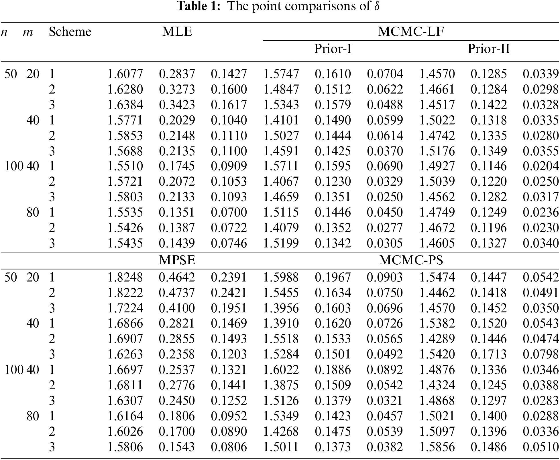
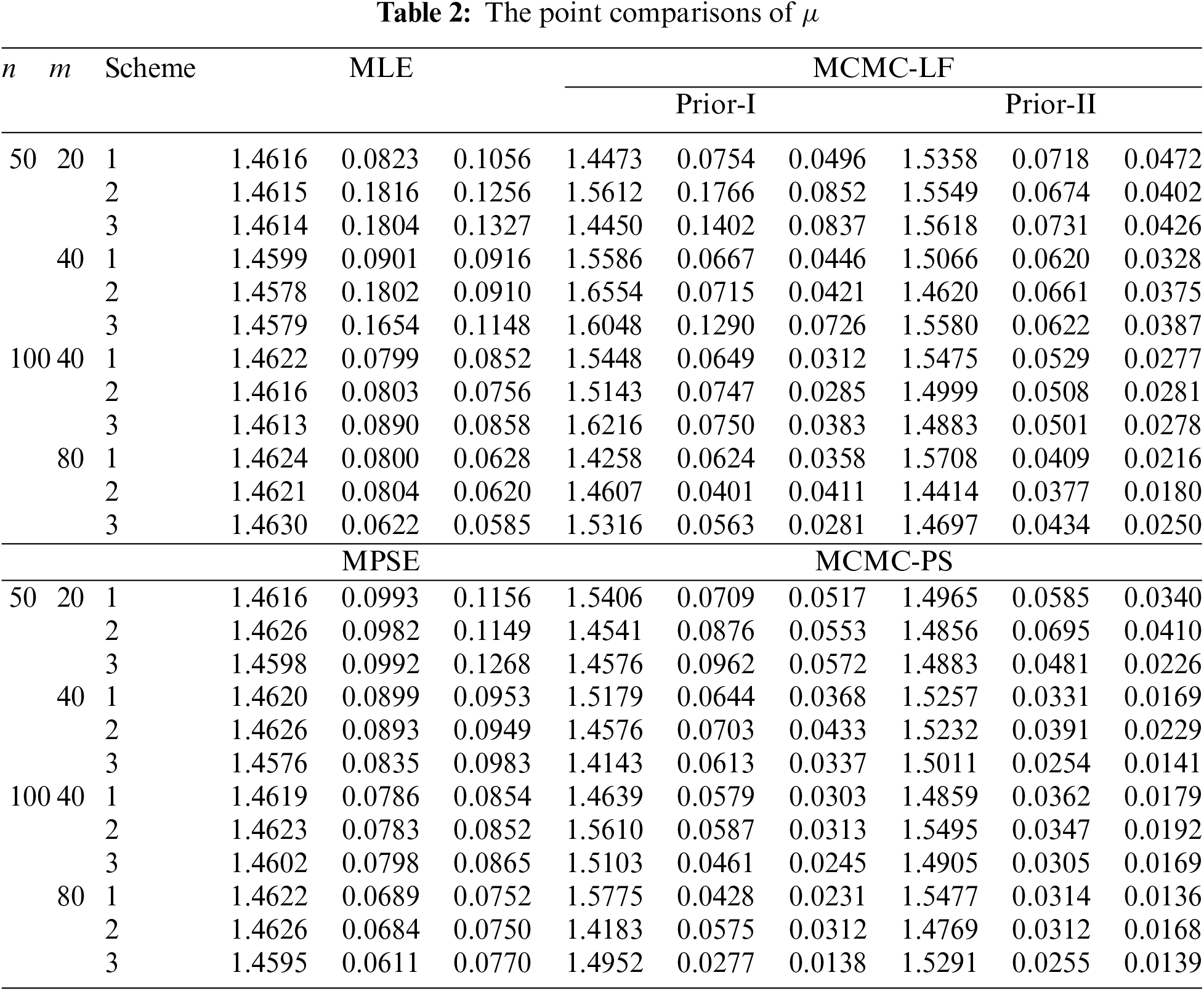
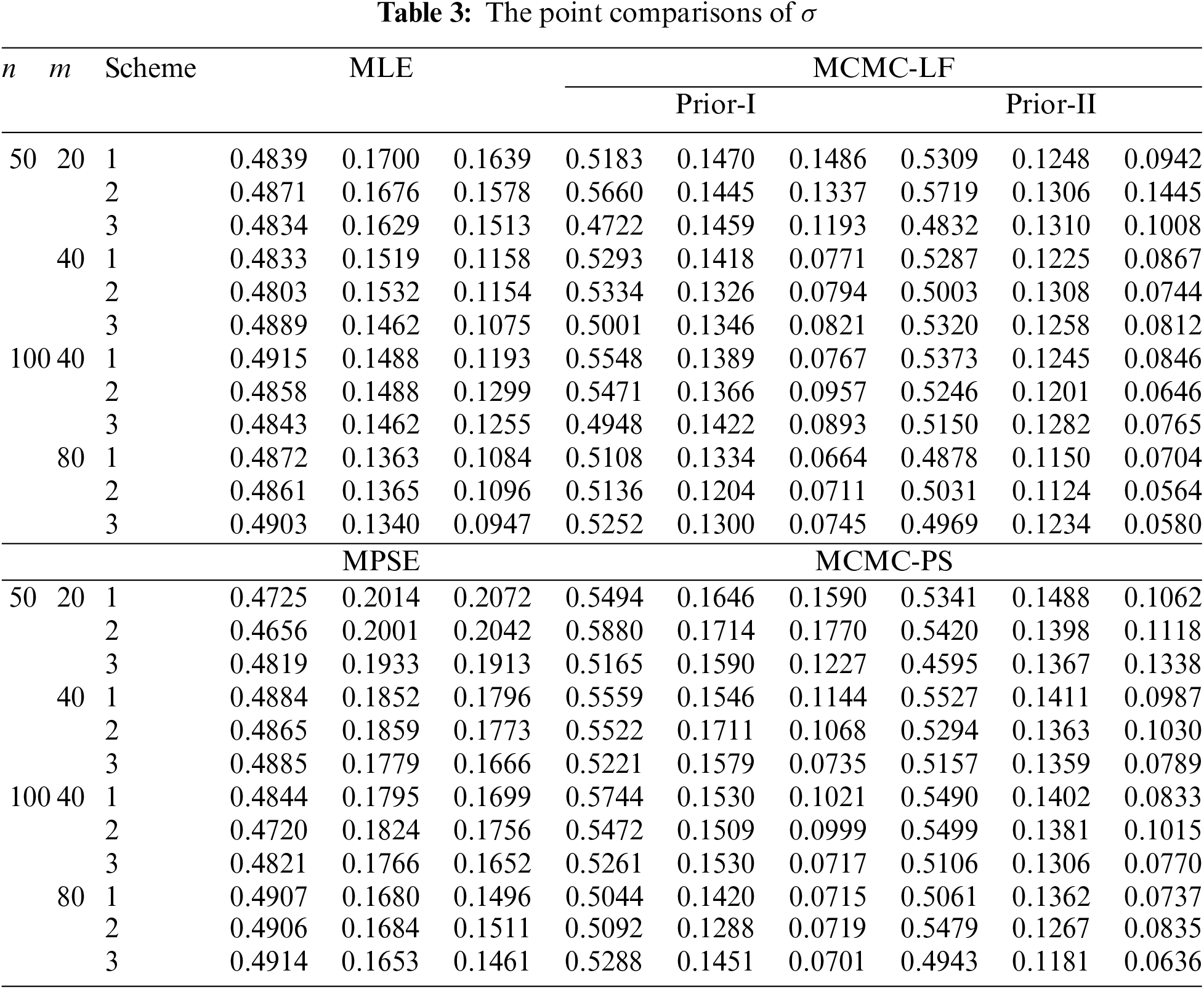
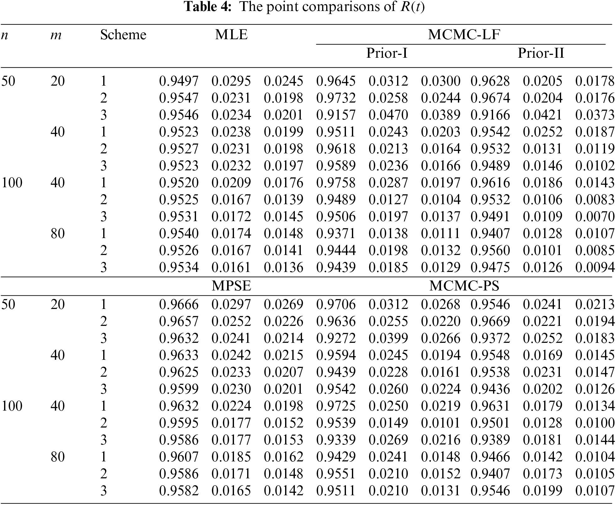
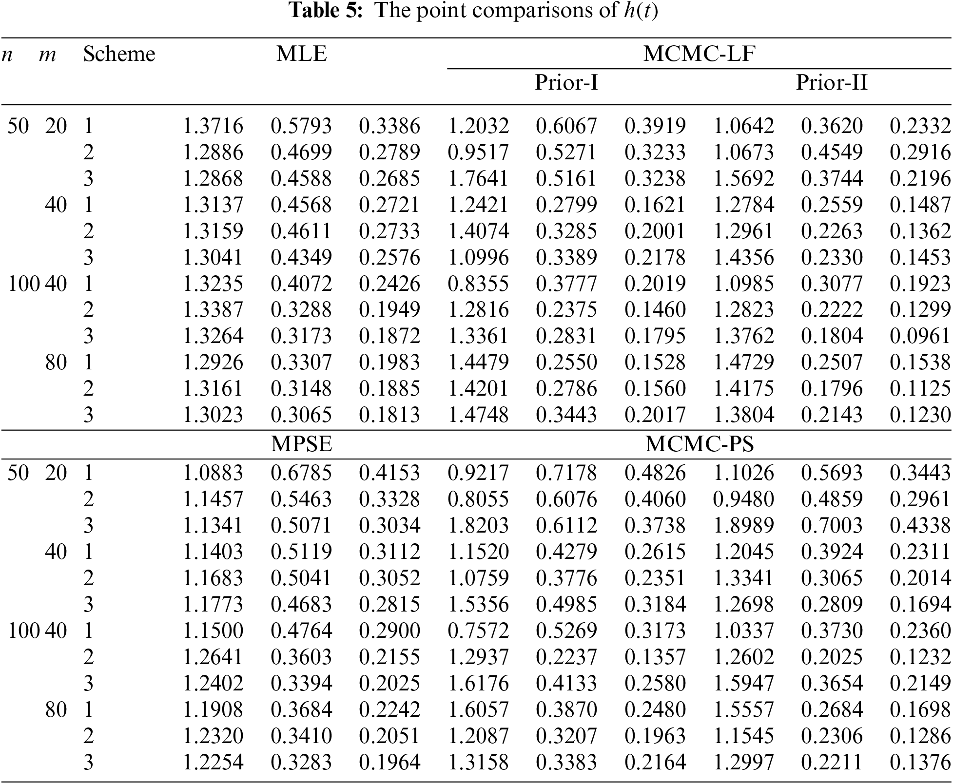
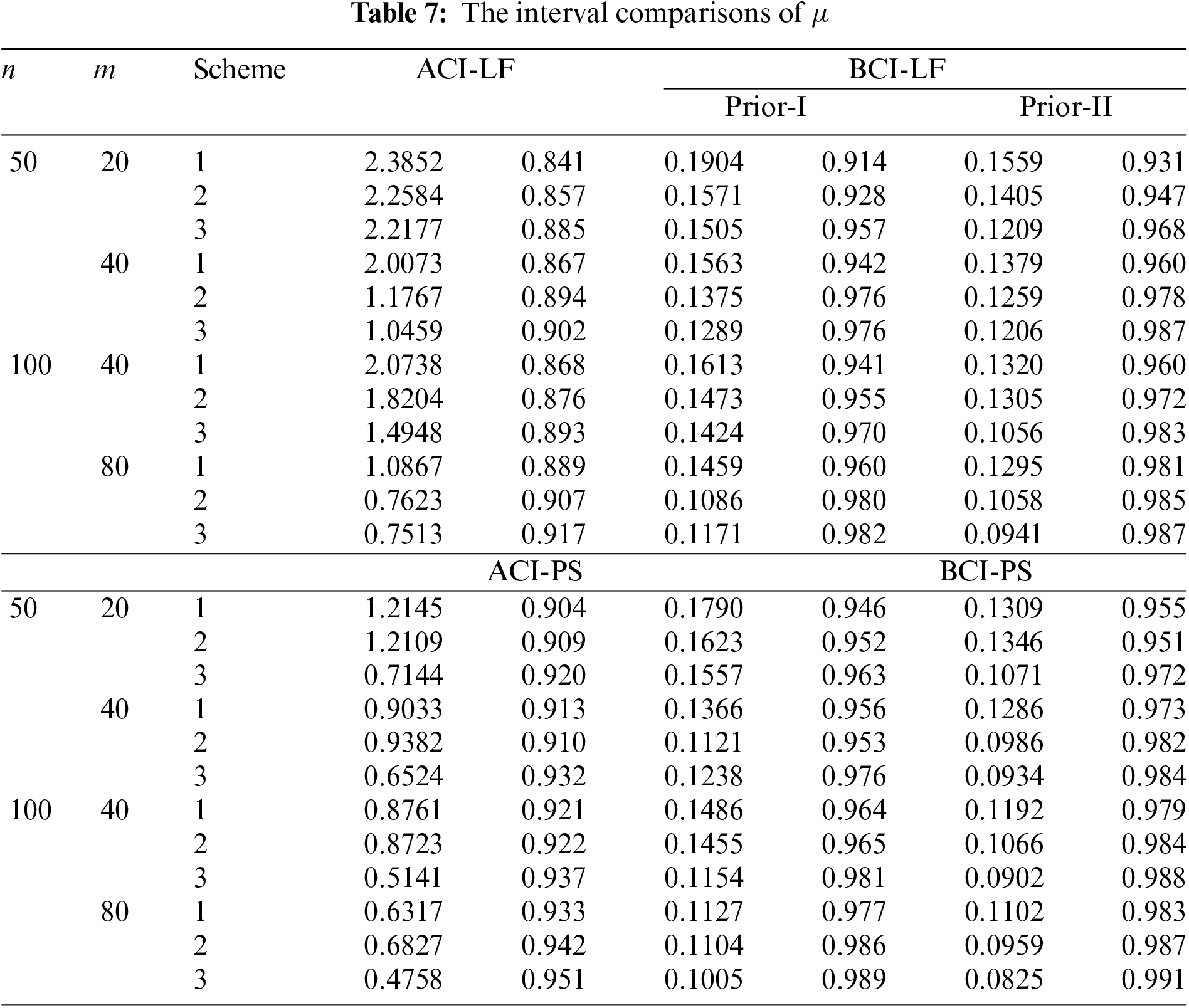
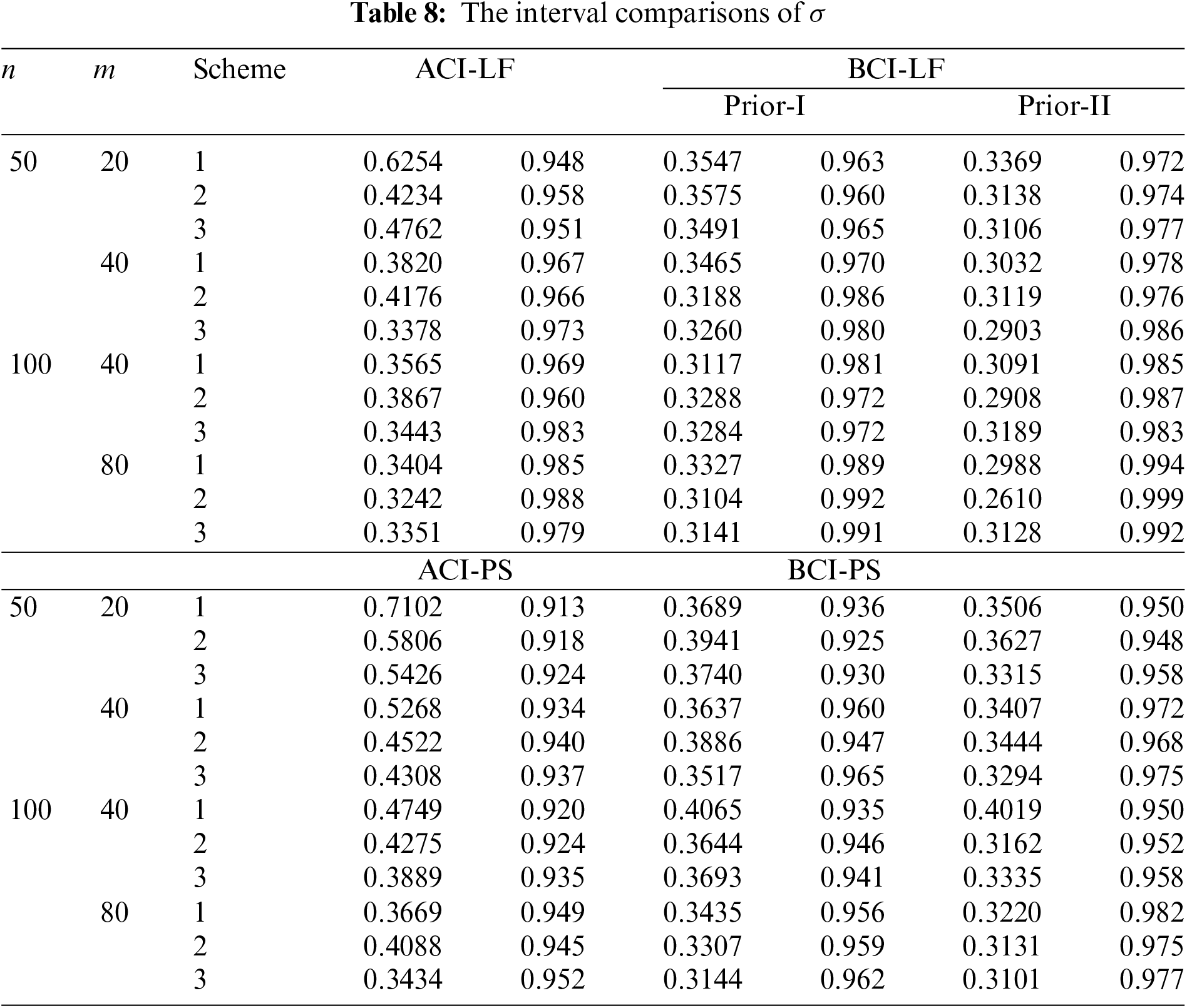
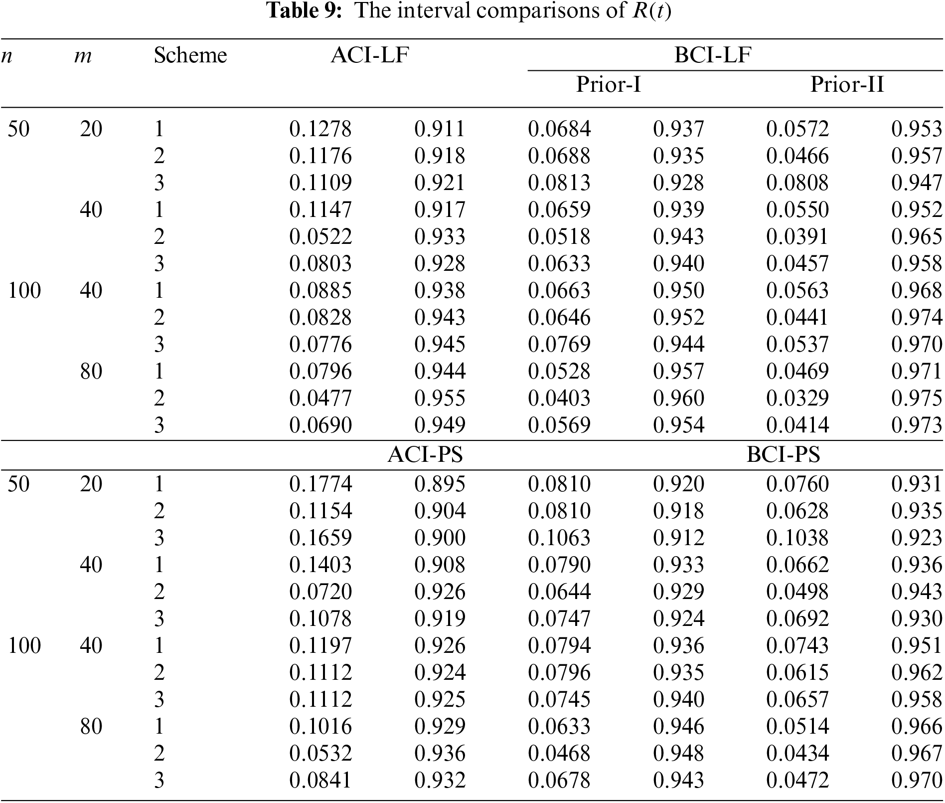
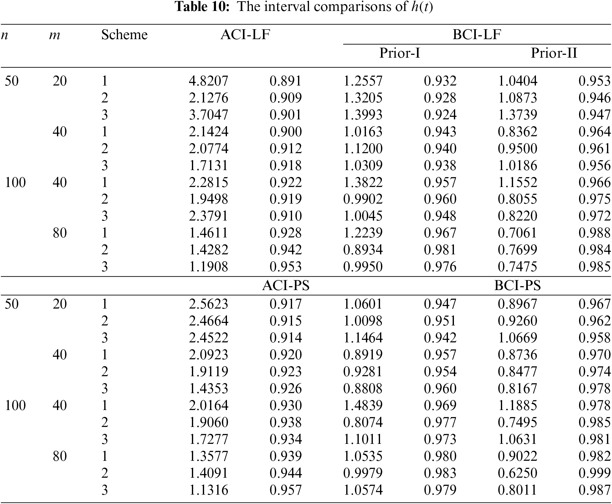
The performances of the point theoretical results of δ, μ, σ, R(t), or h(t) are examined in terms of their values obtained by root-mean-squared-errors (RMSE) and mean-relative-absolute-bias (MRAB). In addition, when ρ=5%, the interval comparison is made based on average interval length (AIL) and coverage-percentage (CP). Taking ϑ1=δ, ϑ2=μ, ϑ3=σ, ϑ4=R(t), and ϑ5=h(t), the average point estimates (APEs) along with their RMSEs, MRABs, AILs, and CPs of ϑι, ι=1,…,5, are obtained using the following formulae, respectively, as

APE(ϑι)=11000∑j=11000ϑ^ι(j),RMSE(ϑι)=11000∑j=11000(ϑ^ι(j)−ϑι)2,MRAB(ϑι)=11000∑j=110001ϑι|ϑ^ι(j)−ϑι|,AIL(ϑι)=11000∑j=11000(U(ϑ^ι(j))−L(ϑ^ι(j))),andCP(ϑι)=11000∑j=110001(Lϑ^ι(j);Uϑ^ι(j))(ϑι),

where ϑ^ι(j) denotes the offered estimate of ϑι, 1(⋅) is the indicator operator, L(ϑ^ι(j)) denotes the lower interval bound, and U(ϑ^ι(j)) denotes the upper interval bound.

All calculations are performed in R with the ‘coda’ (proposed by Plummer et al. [15]) and ‘maxLik’ (by Henningsen et al. [16]) packages. Tables 1–5 list the APEs, RMSEs, and MRABs of each unknown subject in the first, second, and third columns, respectively. Meanwhile, in Tables 6–10, the AILs and CPs of each unknown subject are reported in the first and second columns, respectively. For distinction, using LF (as an example), we abbreviate the Bayes estimates MCMC using LF-based, ACI using LF-based, and BCI using LF-based as MCMC-LF, ACI-LF, and BCI-LF, respectively. From Tables 1–10, regarding the lowest values of RMSE, MRAB, and AIL, as well as the highest values of CP, we can make the following observations:

•   In general, the proposed point (or interval) estimates of δ, σ, R(t), or h(t) showed good behavior.

•   As n (or m) increases or ∑i=1mRi decreases, the accuracy of all acquired estimates becomes better.

•   Comparing the proposed point approaches, it is clear that:

–   The MLE (or MCMC-LF) of δ, σ, R(t), and h(t) performed better compared to those obtained from the PS (or MCMC-PS) approach.

–   The performance of μ behaved better via the PS (or MCMC-PS) approach compared to others.

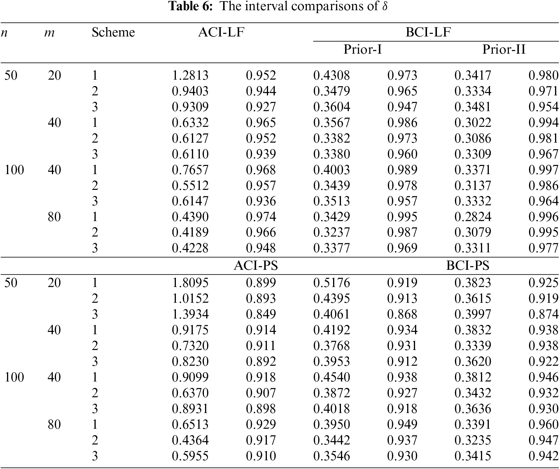
•   Comparing the proposed interval approaches, it is clear that:

–   The ACI-LF estimates of δ, σ, and R(t) have overall lower AILs and higher CPs compared to those obtained using the ACI-PS approach.

–   The AILs of ACI-PS estimates of μ and h(t) have worked effectively compared to those developed from the ACI-LF approach.

•   The CPs of the BCI estimates are (in most cases) greater than the specified nominal level, while the ACI estimates are lower (or closer) to the specified nominal level.

•   Due to the availability of gamma priors, Bayes’ MCMC-LF (or MCMC-PS) estimates of all unknown parameters outperform ML (or MPS) estimates. The same comment is also drawn in the context of comparing the BCI-LF (or BCI-PS) with the ACI-LF (or ACI-PS).

•   Obviously, the variance of Prior-II is less than that of Prior-I. Therefore, all Bayes estimates of all unknown parameters developed from Prior-II using LF (or PS) data outperform those obtained based on other methods.

•   Comparison of the proposed Scheme-1 (first stage) and Scheme-3 (last stage), it is clear that the point estimates of δ, μ, and σ via the LF (using Scheme-1) and via the PS (using Scheme-3) behaved better than others.

•   Regarding the interval estimates of δ, μ, and σ, the associated asymptotic/credible interval estimates become better under Scheme-3, in most situations, compared to others.

•   As a tip, to obtain accurate estimates of any unknown life parameter when the proposed censored data are present, the experimenter should record an appropriate effective sample size, taking into account the total cost of the test.

•   To sum up, the Bayes M-H procedure is recommended to study the unknown parameters of life of the IGG model in the presence of PT2C data.

6  Optimum PT2C

The previous sections dealt with the derivation of point and interval estimations, using both frequentist and Bayesian MCMC estimations, for the parameters of life of the IGG distribution when samples are gathered from the PT2C strategy. Following Ng et al. [17], when the design of removal items R is fixed in advance as well as n (total test items) and m (effective sample) are pre-specified, one can choose the optimal R=(R1,R2,…,Rm) censoring scheme.

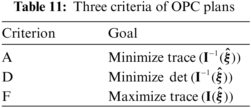
Thus, to select the optimal progressive censoring (OPC) plan, Table 11 reports common criteria for this purpose. Regarding the A-and D-optimality criteria, our objective is to reduce the trace and determinant values of estimated variances and covariances developed from the LF and PS methods. Further, the goal of F-optimality is to maximize the observed values of the Fisher matrices in relation to the MLE (or MPSE) (say, ξ^) of the unknown parameter(s) (say ξ) being considered. The OPC plan that offers more information should correspond to the lowest A and D values and the largest F value; see, for example, Elshahhat et al. [18], Elshahhat et al. [19], among others.

7  Diesel Engine Data Analysis

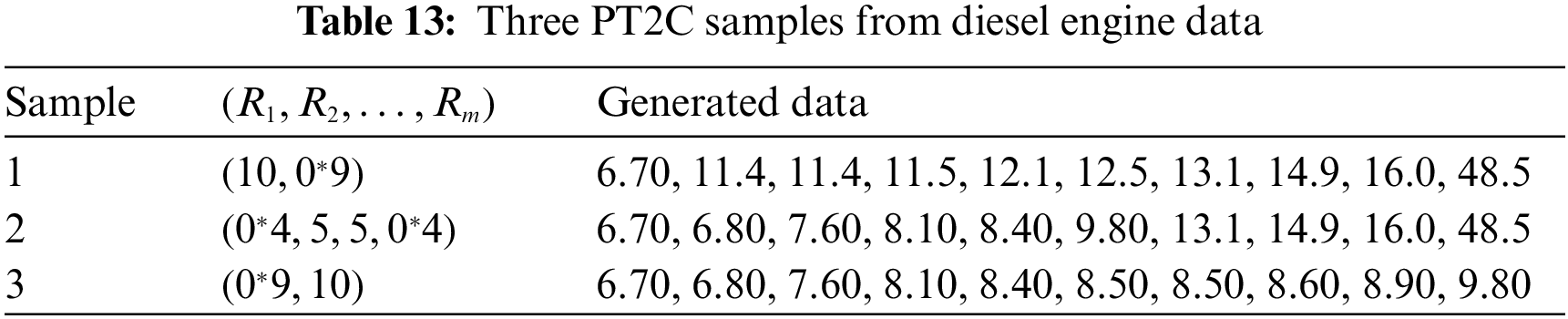
This section analyzes a useful real data set consisting of the failure times (in weeks) of 20 mechanical components of a diesel engine to demonstrate the performance of the proposed methodologies; see Murthy et al. [20]. For computational convenience, we multiply each original data unit by one hundred, and the new transformed data set is: 6.70, 6.80, 7.60, 8.10, 8.40, 8.50, 8.50, 8.60, 8.90, 9.80, 9.80, 11.4, 11.4, 11.5, 12.1, 12.5, 13.1, 14.9, 16.0, and 48.5.

First, the IGG distribution is fitted to the complete diesel engine data with eleven inverted lifetime distributions (for x>0 and δ,μ,σ>0) as competitors, namely:

(1)   Generalized inverted Gompertz (GIG(δ,μ,σ)) by Elshahhat et al. [21].

(2)   Alpha-power inverse-Weibull (APIW(δ,μ,σ)) by Basheer [22].

(3)   Generalized inverse-Weibull (GIW(δ,μ,σ)) by De Gusmão et al. [23].

(4)   Exponentiated inverted-Weibull (EIW(μ,σ)) by Flaih et al. [24].

(5)   Generalized inverted-exponential (GIE(μ,σ)) by Abouammoh et al. [25].

(6)   Generalized inverted half-logistic (GIHL(μ,σ)) by Potdar et al. [26].

(7)   Inverted exponentiated Rayleigh (IER(μ,σ)) by Ghitany et al. [27].

(8)   Inverted Nadarajah–Haghighi (INH(μ,σ)) by Tahir et al. [28].

(9)   Inverted Gompertz (IGo(μ,σ)) by Eliwa et al. [29].

(10)   Inverse-Weibull (IW(μ,σ)) by Keller et al. [30].

(11)   Inverse gamma (IG(μ,σ)) by Glen [31].

To evaluate the feasibility of the IGG model in comparison with other popular models, several information measures are implemented, namely: (i) Kolmogorov-Smirnov (KS) statistic (with its p-value); (ii) Anderson-Darling (AD); (iii) Cramer von Mises (CvM); (iv) estimated negative log-likelihood (ENL); (v) Akaike information (AI); (vi) consistent Akaike information (CAIC); and (vii) Hannan-Quinn information (HQI).

The MLEs (with their standard-errors (SEs)) of δ, μ, and σ as well as the evaluated information criteria are provided in Table 12. It shows that the IGG distribution has the greatest p-value and the lowest values for other statistics, thus the IGG model fits the diesel engine data set quite satisfactorily and is the best choice among others. Moreover, the quantile–quantile (Q–Q) plots for the competitive distributions are displayed in Fig. 3. It also confirms the same findings as displayed in Table 12.

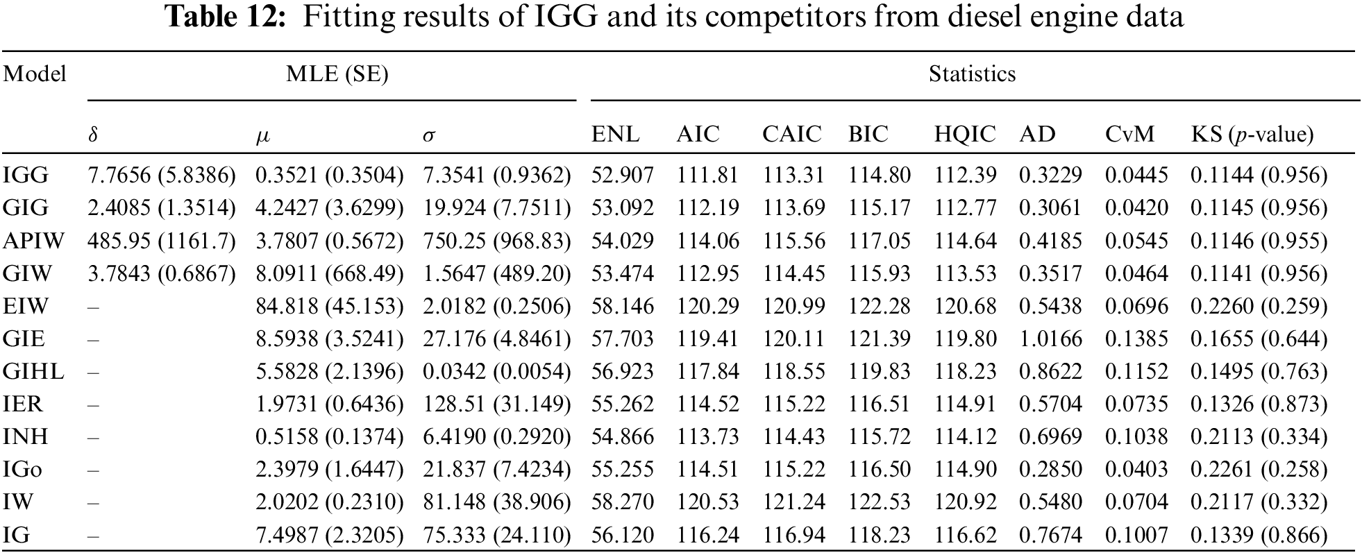
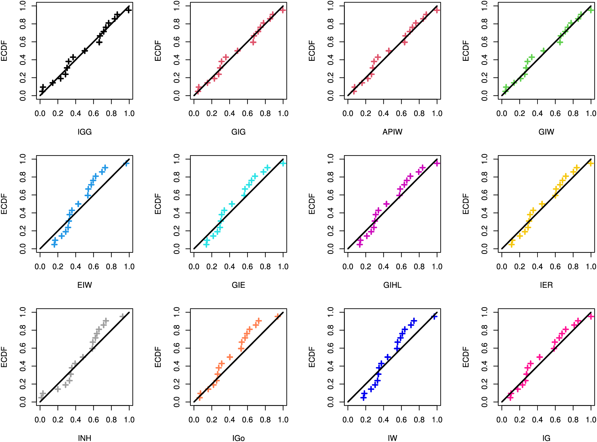
Figure 3: The Q–Q diagrams of IGG and its competitors from diesel engine data

To capture the behavior of the estimated PDFs and CDFs of the IGG and its competitive distributions using the diesel engine data, we have provided two plots: (a) representing the histogram and the fitted densities and (b) representing the fitted/empirical reliability lines; see Fig. 4. It demonstrates that the IGG distribution reflects the overall structure of the histograms and confirms the numerical results presented here.

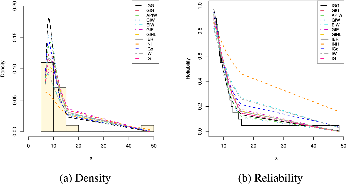
Figure 4: Fitted densities and reliability lines of IGG and its competitors from diesel engine data

Using the complete diesel engine data, for different choices of R, three PT2C samples (with m=10) are obtained; see Table 13. The scheme R=(1,0,0,0,1) (as an example) is referred to as R=(1,0∗3,1) for simplicity. For each PT2C data, the point and interval estimators of δ, μ, σ, R(t), and h(t) (at t=10) are obtained; see Tables 14 and 15, respectively. Since we have no prior information about IGG (Υ), the Bayesian results are approximated using the M-H algorithm based on gamma improper priors, i.e., ai=bi=0, i=1,2,3. Here, to perform our calculations, we set all hyperparameters values to 0.001. To run the MCMC sampler, the initial guess of δ, μ, or σ is taken as MLE (or MPSE), and then the first 5000 (of 30,000) iterations are taken as burn-in.

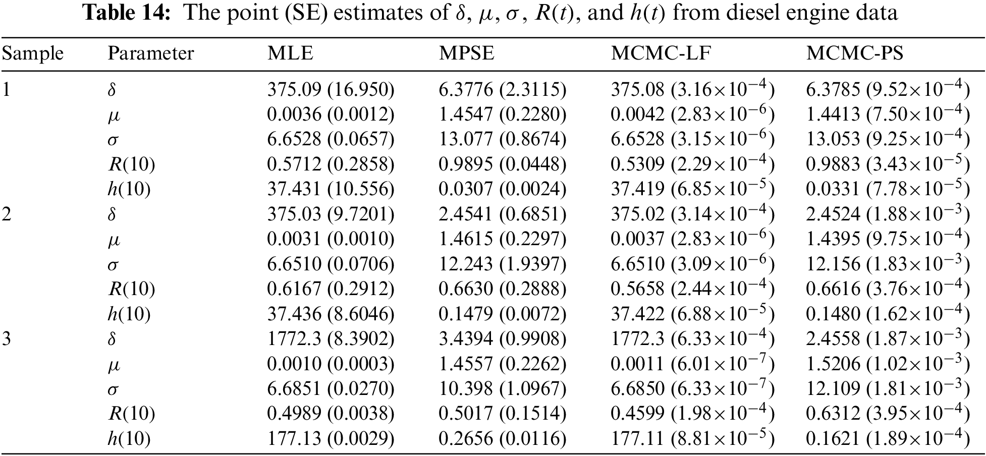
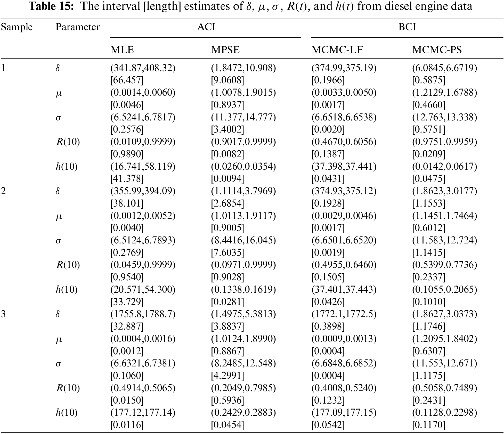
Tables 14 and 15 indicate that the computed estimates of δ, μ, σ, R(t), or h(t) based on both MCMC approaches performed satisfactorily than those obtained based on classical approaches with respect to minimum standard-error and interval length values. Trace diagrams of δ, μ, σ, R(t), and h(t) are plotted; see Fig. 5. For each sup-plot in Fig. 5, the sample average and 95% BCI bounds are displayed with solid and dashed horizontal lines, respectively. Using the Gaussian kernel when the sample average is plotted as a vertical dash-dotted line, Fig. 6 displays the estimates with their histograms of δ, μ, σ, R(t), and h(t). It indicates that the simulated estimates (from MCMC-LF or MCMC-PS) of δ, μ, and σ are fairly symmetrical. It also shows the simulated estimates of R(t) and h(t) are fairly symmetrical (using MCMC-LF) and are also close to being negatively and positively skewed, respectively (using MCMC-PS).

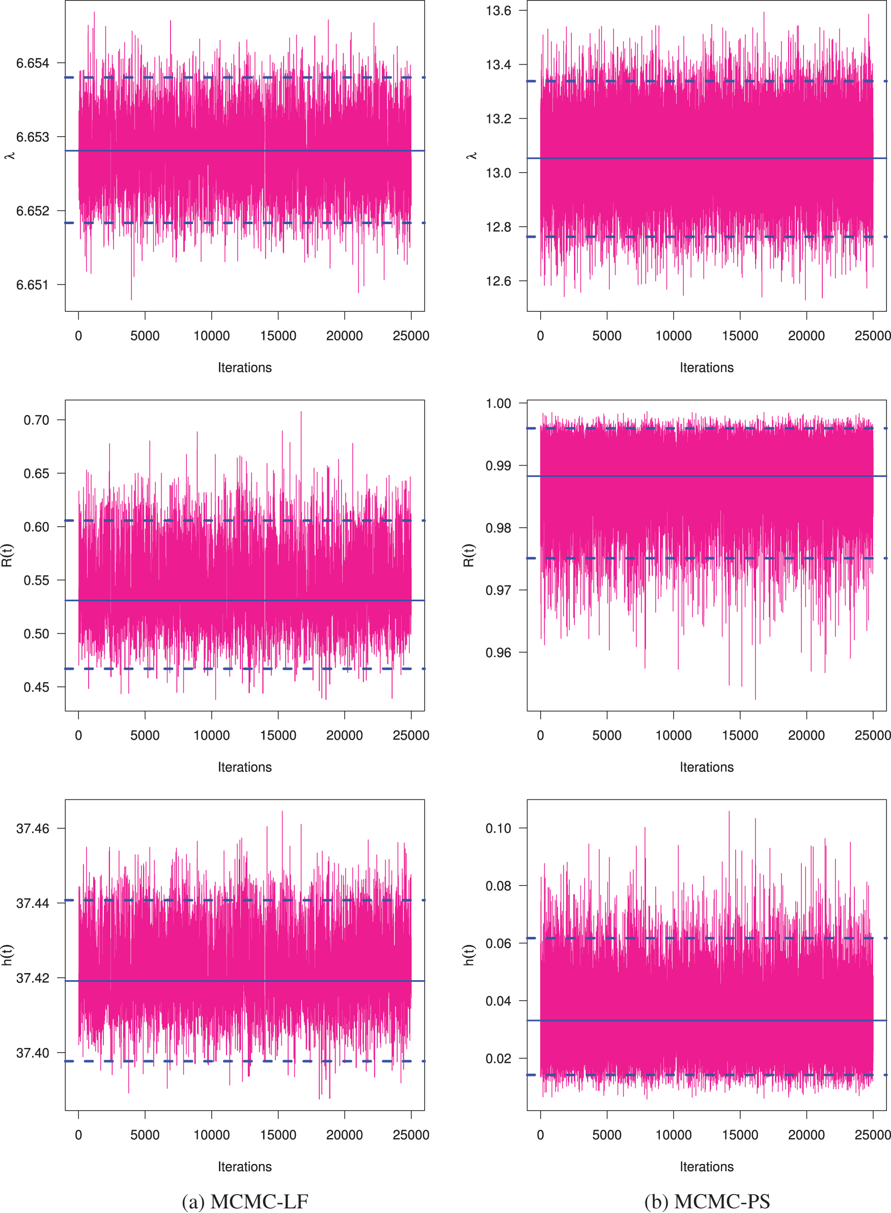
Figure 5: Trace plots of δ, μ, σ, R(t), and h(t) from diesel engine data

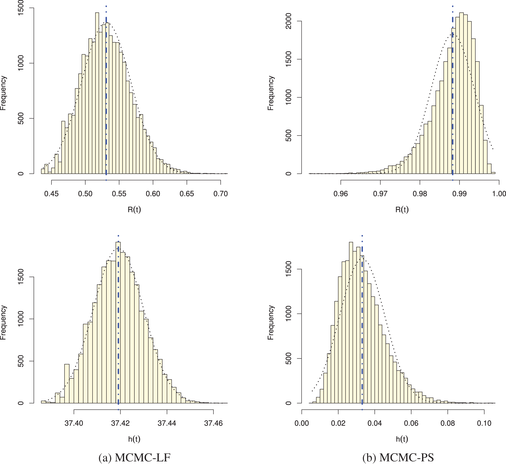
Figure 6: Posterior histograms of δ, μ, σ, R(t), and h(t) from diesel engine data

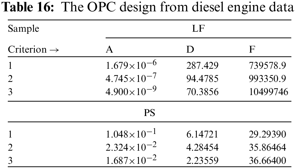
Now, using Table 13, the selection of the OPC plan is explored. So, from (10) and (16), the criteria A, D, and F are evaluated; see Table 16. It shows that the scheme R=(0∗9,10) used in Sample 3 is the best PT2C compared to others. Clearly, the OPC plan proposed here supports our findings reported in Section 5.

8  Concluding Remarks

In this paper, various estimates of the inverted generalized gamma parameters δ, μ, σ, R(t), and h(t) have been investigated through the maximum likelihood and maximum product of spacings, and Bayes methods based on data sets collected from progressively Type-II censoring. In addition, the asymptotic confidence intervals of the same unknown quantites have been obtained based on the maximum likelihood and maximum product of spacing methods, as well as the Bayes’ credible intervals have been obtained based on Bayesian approaches as well. The Monte Carlo results show that, as expected, the Bayesian-based estimates behave satisfactorily when compared with frequentist alternatives. An ideal progressive strategy has been suggested using several metrics. To confirm the practical applicability of our calculations, a real-world data set containing mechanical components of diesel engines has been examined. We recently recommended a Bayes MCMC setup using MPS-based. As future work, it would be better to extend the proposed inferential techniques to other real-life domains such as medicine, physics, chemistry, etc.

Acknowledgement: The authors would desire to express their thanks to the editor and the three anonymous referees for useful suggestions and valuable comments. The authors would also like to express their full thanks to the Deanship of Scientific Research and Libraries, Princess Nourah bint Abdulrahman University, through the Program of Research Project Funding after Publication, Grant No. (RPFAP-34-1445) for supporting this project.

Funding Statement: This research project was funded by the Deanship of Scientific Research and Libraries, Princess Nourah bint Abdulrahman University, through the Program of Research Project Funding after Publication, Grant No. (RPFAP-34-1445).

Author Contributions: The authors confirm contribution to the paper as follows: study conception and design: Refah Alotaibi, Sanku Dey, Ahmed Elshahhat; data collection: Refah Alotaibi, Ahmed Elshahhat; analysis and interpretation of results: Ahmed Elshahhat; draft manuscript preparation: Refah Alotaibi, Sanku Dey. All authors reviewed the results and approved the final version of the manuscript.

Availability of Data and Materials: The data that support the findings of this study are available within the paper.

Conflicts of Interest: The authors declare that they have no conflicts of interest to report regarding the present study.

References

1. Louzada F, Ramos PL, Nascimento D. The inverse Nakagami-m distribution: a novel approach in reliability. IEEE Trans Reliab. 2018;67(3):1030–42. [Google Scholar]

2. Hoq AKMS, Ali M. Estimation of parameters of a generalized life testing models. J Stat Res. 1974;9:67–79. [Google Scholar]

3. Balakrishnan N, Aggarwala R. Progressive censoring theory, methods and applications. Boston, MA, USA: Birkhäuser; 2000. [Google Scholar]

4. Cheng RCH, Amin NAK. Estimating parameters in continuous univariate distributions with a shifted origin. J R Stat Soc Series B. 1983;45(3):394–403. [Google Scholar]

5. Ranneby B. The maximum spacing method. An estimation method related to the maximum likelihood method. Scand J Stat. 1984;11(2):93–112. [Google Scholar]

6. Zhu T. Statistical inference of Weibull distribution based on generalized progressively hybrid censored data. J Comput Appl Math. 2020;371:112705. [Google Scholar]

7. Jeon YE, Kang SB, Seo JI. Maximum product of spacings under a generalized Type-II progressive hybrid censoring scheme. Commun Stat Appl Methods. 2022;29(6):665–77. [Google Scholar]

8. Nassar M, Dey S, Wang L, Elshahhat A. Estimation of Lindley constant-stress model via product of spacing with Type-II censored accelerated life data. Commun Stat Simul Comput. 2024;53(1):288–314. [Google Scholar]

9. Nassar M, Alotaibi R, Elshahhat A. E-Bayesian estimation using spacing function for inverse Lindley adaptive Type-I progressively censored samples: comparative study with applications. Appl Bionics Biomech. 2024;2024(1):5567457. [Google Scholar] [PubMed]

10. Anatolyev S, Kosenok G. An alternative to maximum likelihood based on spacings. Econom Theory. 2005;21(2):472–6. [Google Scholar]

11. Ramos PL, Mota AL, Ferreira PH, Ramos E, Tomazella VL, Louzada F. Bayesian analysis of the inverse generalized gamma distribution using objective priors. J Stat Comput Simul. 2021;91(4):786–816. [Google Scholar]

12. Greene WH. Econometric analysis. 7th ed. Upper Saddle River, New Jersey: Pearson Prentice-Hall; 2012. [Google Scholar]

13. Balakrishnan N, Cramer E. The art of progressive censoring. Birkhäuser, New York: Springer; 2014. [Google Scholar]

14. Kundu D. Bayesian inference and life testing plan for the Weibull distribution in presence of progressive censoring. Technometrics. 2008;50(2):144–54. [Google Scholar]

15. Plummer M, Best N, Cowles K, Vines K. Coda: convergence diagnosis and output analysis for MCMC. R News. 2006;6(1):7–11. [Google Scholar]

16. Henningsen A, Toomet O. maxLik: a package for maximum likelihood estimation in R. Comput Stat. 2011;26(3):443–58. [Google Scholar]

17. Ng HKT, Chan PS, Balakrishnan N. Optimal progressive censoring plans for the Weibull distribution. Technometrics. 2004;46:470–81. [Google Scholar]

18. Elshahhat A, Nassar M. Bayesian survival analysis for adaptive Type-II progressive hybrid censored Hjorth data. Comput Stat. 2021;36(3):1965–90. [Google Scholar]

19. Elshahhat A, Abu El Azm WS. Statistical reliability analysis of electronic devices using generalized progressively hybrid censoring plan. Qual Reliab Eng Int. 2022;38(2):1112–30. doi:10.1002/qre.3058. [Google Scholar] [CrossRef]

20. Murthy DNP, Xie M, Jiang R. Weibull models. In: Wiley series in probability and statistics. Hoboken: Wiley; 2004. [Google Scholar]

21. Elshahhat A, Aljohani HM, Afify AZ. Bayesian and classical inference under Type-II censored samples of the extended inverse Gompertz distribution with engineering applications. Entropy. 2021;23(12):1578. doi:10.3390/e23121578. [Google Scholar] [PubMed] [CrossRef]

22. Basheer AM. Alpha power inverse Weibull distribution with reliability application. J Taibah Univ Sci. 2019;13(1):423–32. doi:10.1080/16583655.2019.1588488. [Google Scholar] [CrossRef]

23. De Gusmão FR, Ortega EM, Cordeiro GM. The generalized inverse Weibull distribution. Stat Pap. 2011;52(3):591–619. doi:10.1007/s00362-009-0271-3. [Google Scholar] [CrossRef]

24. Flaih A, Elsalloukh H, Mendi E, Milanova M. The exponentiated inverted Weibull distribution. Appl Math Inf Sci. 2012;6:167–71. [Google Scholar]

25. Abouammoh AM, Alshingiti AM. Reliability estimation of generalized inverted exponential distribution. J Stat Comput Simul. 2009;79(11):1301–15. doi:10.1080/00949650802261095. [Google Scholar] [CrossRef]

26. Potdar KG, Shirke DT. Inference for the parameters of generalized inverted family of distributions. ProbStat Forum. 2013;6:18–28. [Google Scholar]

27. Ghitany ME, Tuan VK, Balakrishnan N. Likelihood estimation for a general class of inverse exponentiated distributions based on complete and progressively censored data. J Stat Comput Simul. 2014;84(1):96–106. doi:10.1080/00949655.2012.696117. [Google Scholar] [CrossRef]

28. Tahir MH, Cordeiro GM, Ali S, Dey S, Manzoor A. The inverted Nadarajah-Haghighi distribution: estimation methods and applications. J Stat Comput Simul. 2018;88(14):2775–98. doi:10.1080/00949655.2018.1487441. [Google Scholar] [CrossRef]

29. Eliwa MS, El-Morshedy M, Ibrahim M. Inverse Gompertz distribution: properties and different estimation methods with application to complete and censored data. Ann Data Sci. 2019;6(2):321–39. doi:10.1007/s40745-018-0173-0. [Google Scholar] [CrossRef]

30. Keller AZ, Goblin MT, Farnworth NR. Reliability analysis of commercial vehicle engine. Reliab Eng. 1985;10(1):15–25. doi:10.1016/0143-8174(85)90039-3. [Google Scholar] [CrossRef]

31. Glen AG. On the inverse gamma as a survival distribution. J Qual Technol. 2011;43(2):158–66. doi:10.1080/00224065.2011.11917853. [Google Scholar] [CrossRef]

Appendix A: Fisher-LF Elements

Differentiating (6) with respect to the unknown parameters δ, μ and σ, the elements of the observed Fisher information matrix via LF can be expressed as

ℓ11=∂2ℓ∂δ2=−mδ2−∑i=1m(σxi−1)δ(ln⁡(σxi−1))2+∑i=1mRiψi(δ′δ′),

ℓ22=∂2ℓ∂μ2=−nη′(μ)+∑i=1mRiψi(μ′μ′),

ℓ33=∂2ℓ∂σ2=−δσ2[mμ+(δ−1)∑i=1m(σxi−1)δ]+∑i=1mRiψi(σ′σ′),

ℓ12=∂2ℓ∂δ∂μ=mln⁡σ−∑i=1mln⁡xi+∑i=1mRiψi(δ′μ′),

ℓ13=∂2ℓ∂δ∂σ=1σ[mμ−∑i=1m(σxi−1)δ[1+δln⁡(σxi−1)]]+∑i=1mRiψi(δ′σ′),

and

ℓ23=∂2ℓ∂μ∂σ=mδσ+∑i=1mRiψi(μ′σ′),

where η′(μ)=dη(μ)/dμ is the trigamma function,

ψi(δ′δ′)=∂2∂δ2ln⁡γ(μ,(σxi−1)δ)=ψi−2(σxi−1)δμ(ln⁡(σxi−1 ))2exp⁡(−(σxi−1)δ),

ψi(μ′μ′)=∂2∂μ2ln⁡γ(μ,(σxi−1)δ)=ψi−2∫0(σxi−1)δwμ−1(ln⁡(w))2e−wdw,

ψi(σ′σ′)=∂2∂σ2ln⁡γ(μ,(σxi−1)δ)=ψi−2(δσ)2(σxi−1)δμexp⁡(−(σxi−1)δ)[μ−δ−1−(σxi−1)δ],

ψi(δ′μ′)=∂2∂δ∂μln⁡γ(μ,(σxi−1)δ)=ψi−2δ(σxi−1)δμ(ln⁡(σxi−1 ))2exp⁡(−(σxi−1)δ)

ψi(δ′σ′)=∂2∂δ∂σln⁡γ(μ,(σxi−1)δ)=ψi−2σ−1(σxi−1)δμexp⁡(−(σxi−1)δ)[1+δln⁡(σxi−1 )(μ+(σxi−1)δ)]

and

ψi(μ′σ′)=∂∂σln⁡γ(μ,(σxi−1)δ)=δ2σ(σxi−1)δμln⁡(σxi−1 )exp⁡(−(σxi−1)δ).

Appendix B: Fisher-PS Elements

Differentiating (12) with respect to the unknown parameters δ, μ and σ, the elements of the observed Fisher information matrix via PS can be expressed as

S11=∂2ln⁡S∂δ2 =∑i=1m+1[(ψi−1−ψi)(ψi−1(δ′δ′)−ψi(δ′δ′))−(ψi−1(δ′)−ψi(δ′))2(ψi−1−ψi)2]+∑i=1mRiψi(δ′δ′),