Magneto-Photo-Thermoelastic Excitation Rotating Semiconductor Medium Based on Moisture Diffusivity

1  Introduction

The study of how mechanical and thermal processes interact with one another in a material is known as thermoelasticity. The impact of rotation on material behavior is one of the fascinating features of thermoelasticity. In thermoelasticity, rotation is the result of mechanical or thermal forcing on a solid substance. The rotation might be calculated as part of the solution or specified, depending on the particular situation. For instance, in a thermally induced situation, the moment brought on by the non-uniform thermal strain might create a rotation because of the material’s differential expansion. A torque applied to the solid body in a mechanically generated situation has the potential to spin it. The behavior of materials, especially the distributions of stress and strain, is significantly influenced by rotation in thermoelasticity. Thermal stress, or stress resulting from a temperature differential in the material, is a key idea in this context. The thermal stress distribution of a rotating solid body varies, which may lead to non-uniform deformation and eventual collapse. The impact of rotation on natural frequencies and vibrational modes is a significant additional factor in thermoelasticity. The modes of vibration of the material vary as it rotates, potentially leading to instability or even deterioration of the material’s qualities. As a result, while assessing and creating thermoelastic systems, the influence of rotation must be taken into account.

Diffusion in thermoelasticity refers to the process where mass or heat is transferred between two or more materials due to the differences in temperature and pressure between them [1]. Recently, considerable research has been conducted on the diffusion processes in thermo-elastic materials. This research has focused on understanding the mechanisms that control the diffusion process, as well as the factors that affect the rate of diffusion. One area of intense study has been the effect of defects, such as cracks, pores, and dislocations, on the diffusion process in thermo-elastic materials. Several theoretical models have been proposed to describe the diffusion process in thermo-elastic materials. For example, the Arrhenius model assumes that the rate of diffusion is exponentially dependent on temperature and that the activation energy for diffusion can be estimated based on the energy barrier that must be overcome for diffusion to occur. Another model, the Fickian model, assumes that the speed at which diffusion occurs is directly related to the difference in concentration of the substance being diffused [2]. Overall, Diffusion in thermo-elasticity has improved knowledge of mechanisms. that control the transfer of mass and heat in these materials. The study of material properties and behavior under extreme conditions, as well as the design and development of energy conversion devices, are all significantly affected by this understanding. As research in this area continues, new models and techniques will likely be developed that further enhance our understanding of this complex phenomenon. Szekeres [1,2] investigated how generalized heat transport and moisture interact. According to Gasch et al. [3], changes in temperature and moisture levels might cause more damage than actual loads. To create equations that control the behavior of coupled hygrothermoelasticity. Povstenko [4] used the thermal stresses theories to study the time-fractional telegraph equations in the context of thermoelasticity theory.

In recent years, the photothermal (PT) technique has gained recognition for analyzing the electrical and thermal properties of semiconductor materials. These materials, increasingly important in industries like sensors, solar panels, and advanced medical equipment, are essential for renewable energy production. Semiconductors possess moderate conductivity, and when light energy interacts with them, electrons and holes are stimulated, creating electronic deformations (ED). Thermoelastic deformation (TED) refers to structural alterations caused by the excitation of electrons through light impact, leading to the creation of an electron cloud exhibiting characteristics akin to plasma waves. Heat generated in this process contributes to TED. Researchers have explored innovative methods to study how semiconductor samples react to a laser beam, including sensitivity analysis using photoacoustic spectroscopy. These explorations incorporate the application of thermoelasticity theory as well as the PT theory [5,6]. To ascertain the precise values of temperature, internal displacements, thermal diffusion, and other electrical properties of nano-composite semiconductor materials, PT techniques were applied in several physical experiments [7–10]. Electronic deformation is directly related to changes in the density of free carriers, which are in turn caused by the thermal wave generated by laser or sunlight pulses within the material’s internal structures [11]. In their research, Hobiny et al. [12] examined the phenomenon of PT waves in a limitless medium by utilizing a cylindrical cavity filled with semiconductor material. These topics have been explored in various studies [13,14]. Mahdy et al. [15–18] extensively investigated the concept of photo-thermoelasticity by studying the influence of external elements like magnetic fields and rotation on the interplay of thermal-plasma-elastic waves in semiconductor materials. Wave propagation in a photo-thermoelastic semiconductor medium is studied, together with the effects of humidity, magnetic field, and rotational field.

Sur et al. [19] studied the fibre-reinforced magneto-thermoelastic medium subjected to a moving heat source and took some applications according to the thermal therapy of cancer cells. Changing a material’s temperature can substantially affect its mechanical and thermal properties. Since the expanded theory of thermoelasticity has been the subject of multiple investigations, many researchers have studied the effect of the temperature gradient, which has been largely disregarded in the past [20–24]. Understanding how temperature affects material characteristics is extremely important because we cannot assume that the characteristics of a material remain constant as temperature changes [25]. Since earlier discussions on coupled and uncoupled theories did not match up with practical tests, the thermoelasticity theory was established. This issue was fixed by the novel theory of connected thermoelasticity suggested by Biot [26]. Biot [26] proposed a dynamic theory of thermoelasticity (CD theory) that utilized The Fourier law of heat. The behavior of thermal waves moving at limitless velocities was the focus of his theory. Adding a single relaxation period to the heat equation was an innovative approach introduced by Lord et al. [27]. This was expanded upon by Green et al. [28], who added two relaxation intervals to the heat conduction equation. Multiple studies [29,30] have made use of GL’s proposed generalized thermoelasticity theory. The theory explores how several types of waves behave and interact within a solid medium, including heat waves, electric fields, and mechanical vibrations. Lata et al. [31] investigated the impact of multi-dual-phase-lag heat for isotropic thermoelastic medium according to a couple stress model with two temperature theory. On the other hand, Lata [32] used fractional calculus to study the magneto-thermoelastic rotating material according to GN-II theory. Marin et al. [33] applied a new model according to Some results in Moore-Gibson-Thompson thermoelasticity with biological application for skin tissue. Roy et al. [34] studied the fractional heat order for a thermoelastic medium under the impact of voids according to three-Phase-Lag thermal memory.

This problem is investigated in the context of one-dimensional thermo-elasticity, with special attention paid to the role that mechanical force and the diffusivity of moisture play in the photo-thermal transport process. An answer is found in the research, but only at the free surface of a semi-infinite semiconducting medium. Important physical quantities have analytical solutions found by applying Laplace transforms to the governing equations. Using a powerful programming language, the inversion of the transforms is carried out numerically. The study is completed by numerically and graphically computing several properties, such as normal displacement, normal force stress, moisture concentration, carrier density, and temperature distribution.

2  Basic Equations

Assume that the object being studied is rotating evenly. In such circumstances, the angular velocity can be denoted as Ω_=Ωn_, where n_ is a unit vector describing the axis of rotation. There are two supplementary terms added to the motion equation in the rotating reference frame:

(1) Acceleration of Coriolis’s 2Ω_×u˙_, u_ is the displacement vector.

(2) Centripetal acceleration, Ω_×(Ω_×u_) since motion over time is the only cause.

In a problem that involves only one dimension, every variable is solely dependent on the coordinate x and time t. considered the angular velocity as Ω_=(0, Ω, 0). On the other hand, when there is no rotation, these terms are absent in the medium.

In addition, the magnetic field must be adjusted so that H=H0+h, H⇀=(0, H0, 0) is the initial magnetic field and h(x, y, z) is the magnetic field generated in a way that is aligned with the y-axis. To start our analysis, we will focus on the linearized version of electro-dynamics in which only slow-moving mediums are considered, and there is no consideration for the electric charge density. Here is an application of Maxwell’s equations, which describe the behavior of electromagnetic fields [15,16]:

J⇀=curlh⇀−ε0E⇀˙,(1)

curlE⇀=−μ0H⇀˙,(2)

E⇀=−μ0(u⇀˙×H⇀),(3)

divH⇀=0.(4)

In these equations, we have the magnetic permeability represented by a symbol μ0, the electric permeability represented by a symbol ε0, and the particle velocity of the medium represented by the symbol u⇀˙. We also assume that any small effects of temperature gradients u˙⇀ can be ignored. The equations are written with a dot notation to indicate differentiation to time. Additionally, we can express the components of the vector E⇀ (which is assumed to have the same direction as the current density vector J⇀=(J1, J2, J3)) in terms of displacement. The components of current density are Jx=0, Jy=0 and Jz=∂h∂x+μ0H0ε0u¨ when eliminating the quantities h⇀ and E from Eq. (1).

A medium’s magnetic intensity is a vector whose components are [15]:

Hx=0, Hz=0, Hy=H0+h(x, y, z).(5)

Let’s pretend we have a homogeneous, transversely anisotropic semiconductor material with linear elastic characteristics. Here, we explore this material’s behavior throughout the PT transport stage of its life cycle. We also account for the fact that moisture and plasma-thermal diffusion within the semiconductor material often coincide. In this study, the displacement vector u(rk,t), moisture concentration m(rk,t), temperature distribution T(rk,t), and carrier density distribution (intensity) N(rk,t). The following tensor representation of the equations describes how moisture diffuses in a plasma subjected to thermal-elastic waves [35–37]:

∂N(ri, t)∂t=DEN,ii(ri, t)−N(ri, t)τ+κT(ri, t),(6)

ρCe(DTT,ii(ri, t)+DTmm,ii(ri, t))=ρCe∂T(ri, t)∂t−EgτN(ri, t)+γtT0∂ui,j(ri, t)∂t,(7)

km(Dmm,ii(ri, t)+DmTT,ii(ri, t))=km∂m(ri, t)∂t−EgτN(ri, t)+γmm0Dm∂ui, j(ri, t)∂t.(8)

In this scenario, the effects of Lorentz force and moisture diffusion are factored into the equations of motion for a plasma wave that is subject to both a rotating field and a magnetic field [15,35]:

ρ(u→¨(r, t)+Ω_×(Ω_×u→)+2Ω_×u→˙)=μ∇2u→(r, t)+(μ+λ)∇(∇.u→)−γ∇T−δn∇N−γm∇m+F⇀}.(9)

The following equation describes the displacement and strain tensor:

εij=12(ui, j+uj, i).(10)

The relationship between plasma temperature, displacement, stress, and moisture concentration using a tensor form can be represented as follows [37]:

σij=Cijklεkl−βij(αtT+dnN)−βijmm,i, j, k, l=1, 2, 3.(11)

The equation includes several parameters such as temperature diffusivity DT, the diffusion coefficient of moisture represented by Dm, DTm and DmT the coupled diffusivities. The carrier diffusion coefficient is represented by DE, and the reference moisture and moisture diffusivity are represented by symbols m0 and km, respectively. The tensor Cijkl representing the symmetric isothermal parameters of an elastic medium and the strain tensor is represented by εkl. The material coefficient of moisture concentration is represented βij and βijm, respectively. The thermal activation coupling parameter that is non-zero is κ=∂N0∂TTτ, the equilibrium carrier concentration is denoted by N0 [10,12], κ is disregarded when the temperature is comparatively low. However, in the majority of cases. Assuming that the thermal activation coupling parameter is not zero, we discuss the issue at hand., although it may be neglected in certain cases where the temperature is relatively low. Eg, τ, ρ, μ, λ, and T0 are known as the energy gap, carrier lifetime, density, Lame’s elastic constants, and absolute temperature. Also, γt=(3λ+2μ)αT is the volume thermal expansion, where αT is the linear thermal expansion coefficient, Ce is the specific heat coefficient at constant strain for a solid plate, the conductive deformation potential and valence band difference are represented by δn. The semiconductor’s (in the form of a rod x=±1) elastic surface boundary conditions. Because of the thermal insulation imposed by the surface boundary conditions, closed circuits, isothermal conditions, and stress loads can all be applied without interference. Since the physical variables are independent of the yz-coordinates, all studies are performed along the x-axis. The Lorentz force is represented by F⇀=μ0(J⇀×H⇀) in 1D:

F⇀=μ0(J⇀×H⇀)≡(−μ0H0∂h∂x−ε0μ02H02∂2u∂t2, 0, 0)≡Fxi⇀.(12)

We can define the basic physical quantities in one dimension (1D) using the following expressions [35]:

∂N∂t=DE∂2N∂x2−Nτ+κT,(13)

ρCe(DT∂2T∂x2+DTm∂2m∂x2)=ρCe∂T∂t−EgτN+γtT0∂e∂t,(14)

km(Dm∂2m∂x2+DmT∂2T∂x2)=km∂m∂t−EgτN+γmm0Dm∂e∂t.(15)

The form of the motion Eq. (9) is as follows:

ρ(∂2u∂t2−Ω2u)=(2μ+λ)∂2u∂x2−γ∂T∂x−δn∂N∂x−γm∂m∂x−μ0H0∂h∂x−ε0μ02H02∂2u∂t2,(16)

where γt, m=βαm, T, δn=βdn, β=3μ+2λ, and h=−H0e.

The equation that defines the relationship in one dimension can be expressed as:

σxx=(2μ+λ)∂u∂x−β(αtT+dnN)−γmm=σ.(17)

3  Mathematical Formulation of the Problem

To make it simpler, new simplified variables are introduced that have no units associated with them.

(x′, u′)=(x, u)CTt∗,Ω′=t∗Ω,(T′, N′)=(γtT, δnN)2μ+λ,m′=m,e′=e,t′=tt∗,h′=hρCT2,σ′=σμ(18)

In Eqs. (13)–(17), the dashes are omitted for convenience. Using Eq. (18), when the strain in 1D is e=ux, yields:

(∇2−α1−α2∂∂t)N+ε3T=0,(19)

(∇2−b1∂∂t)T+b2∇2m+b3N−ε1∂e∂t=0,(20)

(∇2−b4∂∂t)m+b5∇2T+b6N−b7∂e∂t=0,(21)

(α∇2−RH∂2∂t2−Ω2)e−∇2T−∇2N−b8∇2m=0.(22)

The stress component in one dimension appears in the non-dimensional form in the following way:

σxx=b9(e−(T+N))−b10m=σ.(23)

where

α1=kt∗DEρτCe, α2=kDEρCe, b1=CT2t∗DT, b2=DTmγtDT(2μ+λ), ε2=αTEgt∗τdnρCe, b3=ε2b1ε1=γt2T0t∗kρ, b4=CT2t∗Dm, b5=DmT(2μ+λ)Dmγt, b6=Eg(2μ+λ)t∗b4kmδnτ, b7=γmm0CT2t∗km,b8=γm2μ+λε3=dnkκt∗αTρCeDE, b9=2μ+λμ, b10=γmμ CT2=2μ+λρ, δn=(2μ+3λ)dn, t∗=kρCeCT2, α=1+μ0H02/(2μ+λ), RH=1+ε0μ02H02/ρ.

The parameters ε3, ε1, and ε2 can be called the thermoelectric coupling parameter, the thermoelastic coupling parameter, and the thermo-energy coupling parameter, respectively.

One way to approach solving an analytical problem involves taking into account certain initial conditions that exhibit homogeneity properties. These conditions can be expressed as follows:

e(x,t)|t=0=∂e(x,t)∂t|t=0=0,T(x,t)|t=0=∂T(x,t)|∂t|t=0=0,m(x,t)|t=0=∂m(x,t)∂t|t=0=0.σ(x,t)|t=0=∂σ(x,t)∂t|t=0=0,N(x,t)|t=0=∂N(x,t)∂t|t=0=0.(24)

4  The Solution to the Problem

Using Laplace transformation, which is a mathematical technique that can be utilized on any function ℑ(x,t), according to its definition:

L(ℑ(x, t))=ℑ¯(x, s)=∫0∞ℑ(x, t)exp⁡(−st)dt.(25)

Using Eq. (25) for the basic five Eqs. (19)–(23), yields:

(D2−α3)N¯+ε3T¯=0,(26)

(D2−α4)T¯+b2D2m¯+b3N¯−α5e¯=0,(27)

(D2−α6)m¯+b5D2T¯+b6N¯−α7e¯=0,(28)

(αD2−α8)e¯−D2T¯−D2N¯−b8Dm¯=0,(29)

σ¯xx=b9(e¯−(T¯+N¯))−b10m¯=σ¯,(30)

where D=ddx, α3=α1+α2s, α4=b1s, α5=sε1, α6=b4s, α7=b7s, α8=RHs2+Ω2.

Eliminating T¯, e¯, N¯ and m¯ between Eqs. (26)–(29), yields:

(D8−Θ1D6+Θ2D4−Θ3D2−Θ4){m¯, N¯, T¯, e¯}(x, s)=0.(31)

where

Θ1=−1(−α+αb2b5){αα3−αb2b5α3+αα4+α5−b5b8α5+αα6−b2α7+b8α7+α8−b2b5α8}Θ2={−αα3α4−α3α5+b5b8α3α5−αα3α6−αα4α6−α5α6+b2α3α7−b8α3α7−b8α4α7−α3α8+b2b5α3α8−α4α8−α6α8+αb3ε3−αb2b7ε3−α5ϵ3+b2α7ε3}(−α+αb2b5),Θ3=−{αα3α4α6+α3α5α6+b8α3α4α7+α3α4α8+α3α6α8+α4α6α8+b7b8α5ε3−αb3α6ε3+α5α6ε3−b3b8α7ε3−b3α8ε3+b2b7α8ε3}(−α+αb2b5),Θ4={−α3α4α6α8+b3α6α8ε3}(−α+αb2b5).},(32)

Using the factorization technique, the original ordinary differential equation (ODE) (31) may be solved, as shown below:

(D2−k12)(D2−k22)(D2−k32)(D2−k42){T¯, e¯, N¯, m¯}(x, s)=0.(33)

where ki2(i=1, 2, 3, 4) stands for the potential roots in the positive actual component when x→∞. Given the problem’s linearity, the solution to equation (ODE) (33) looks like this:

T¯(x,s)=∑i=14Di(s)e−kix.(34)

The other quantities’ solutions can also be stated as:

N¯(x,s)=∑i=14Di′(s)e−kix=∑i=14H1iDi(s)e−kix,(35)

e¯(x,s)=∑i=14Di′′(s)exp⁡(−kix)=∑i=14H2iDi(s)exp⁡(−kix),(36)

m¯(x,s)=∑i=14Di′′′(s)exp⁡(−kix)=∑i=14H3iDi(s)exp⁡(−kix),(37)

σ¯(x,s)=∑i=14Di(4)(s)exp⁡(−kix)=∑i=14H4iDi(s)exp⁡(−kix).(38)

where Di,Di′,Di′′, and Di′′,i=1, 2, 3, 4 vary depending on the parameter and are unknown parameters s. The connection among the unknown parameters Di,Di′,Di′′, and Di′′′ can be obtained When utilizing the primary formulas (26)–(30), which describe the subsequent correlation:

H1i=−ε3mi2−α3,H2i=(b2(b7+b3b8)ki2−b22ki4+(ki2−α4)(−b7b8+ki2−α6)+b3(−ki2+α6))(ki2(α5(−b7b8+ki2−α6)+b2(−ki2α7+b7(αki2−α8)))+b3(α6α(aaki2−α8)+ki2(−αk12+b8α7+α8))),H3i=−((−b3ki2+ki2(ki2−α4))(b7kiα5−b3kiα7)−(b2b3ki2−b7(ki2−α4))(−ki3α5+b3k2(αki2−α8)))((−b3b8ki2+b2ki4)(b7kiα5−b3kiα7)−(−b2b7ki2+b3(ki2−α6))(−ki3α5+b3ki(αki2−α8))),H4i=b9(H2i−(1+H1i))−b10H3i.

In the domain of unknown parameters Di(s), the preceding equations provide us a solution for Laplace’s main variable transform. The boundary conditions will provide us these values.

5  Boundary Conditions

To specify Di(s), consider the following example: an elastic semiconductor material’s outer surface is exposed to various mechanical, plasma, and thermal stresses. In every scenario, the Laplace transforms are employed:

(I) When x=0, a system is thermally isolated, the free surface experiences thermal shock and serves as the isothermal boundary condition:

T¯(0, s)=T0.(39)

Therefore,

∑n=14Di(s)=T0s.(40)

(II) To evaluate the condition of the mechanical normal stress components on the surface when x=0, Laplace transformation is used:

σ¯xx(0, s)=0.(41)

Therefore,

∑i=14{b9(H2i−(1+H1i))−b10H3i}(Di)=0.(42)

(III) When the diffusion of carrier density and the photo-generation during recombination processes are being transported, the plasma boundary condition at the free surface (x=0) can be expressed differently by using the Laplace transform. Here, the plasma condition takes the form of the following:

N¯(0,s)=ƛDeR¯(s).(43)

In contrast, we found the following relationship:

∑i=14H1iDi(x,s)=ƛsDE.(44)

(IV) Free-surface boundary conditions for displacement when x=0.

u¯(0, s)=0.(45)

alternatively, the following relationship was derived:

∑i=14H2ikiDi(x,s)=0.(46)

The equations above use symbols h(t) Z(s) R(s) that indicate the Heaviside unit step function, with a chosen constant ƛ. We can obtain the unknown parameters Di via resolving these equations using the parameters.

6  Transforming the Fourier-Laplace Transforms in Reverse

Laplace transform inversion can be used to derive the dimensionally-free physical fields in the time domain. To get an approximate estimate of the Laplace transform, one can use numerical approaches like the Riemann-sum approximation method [38]. Any function ℑ¯(x,s) in the Laplace domain may be derived as follows:

ℑ(x,t′)=L−1{ℑ¯(x,s)}=12πi∫n−i∞n+i∞exp⁡(st′)ℑ¯(x,s)ds.(47)

In the case of s=n+iM  (n,M ∈R), then the inverted Eq. (47) can be rewritten as:

ℑ(x,t′)=exp⁡(nt′)2π∫−∞∞exp⁡(iβt)ℑ(x,n+iβ)dβ.(48)

Extending the function over a closed interval [0,2t′] with the Fourier series yields the following formula ℑ(x,t′):

ℑ(x,t′)=ent′t′[12ℑ¯(x,n)+Re∑k=1Nℑ¯(x,n+ikπt′)(−1)n].(49)

where Re and i represent the real part and the imaginary unit, respectively, in this case, the sufficient N can be chosen free as a large integer but can be selected in the notation nt′≈4.7 [38].

7  Numerical Results and Discussions

The physical quantities in this problem such as displacement, temperature, moisture concentration, stress distribution, and carrier density are represented by numerical values for a brief duration. Materials are utilized for numerical simulations and SI units and constants are utilized, with software such as MATLAB used to plot the physical constants. Table 1 provides the physical constants of the semiconductor media for Si and Ge, as indicated in references [39–42].

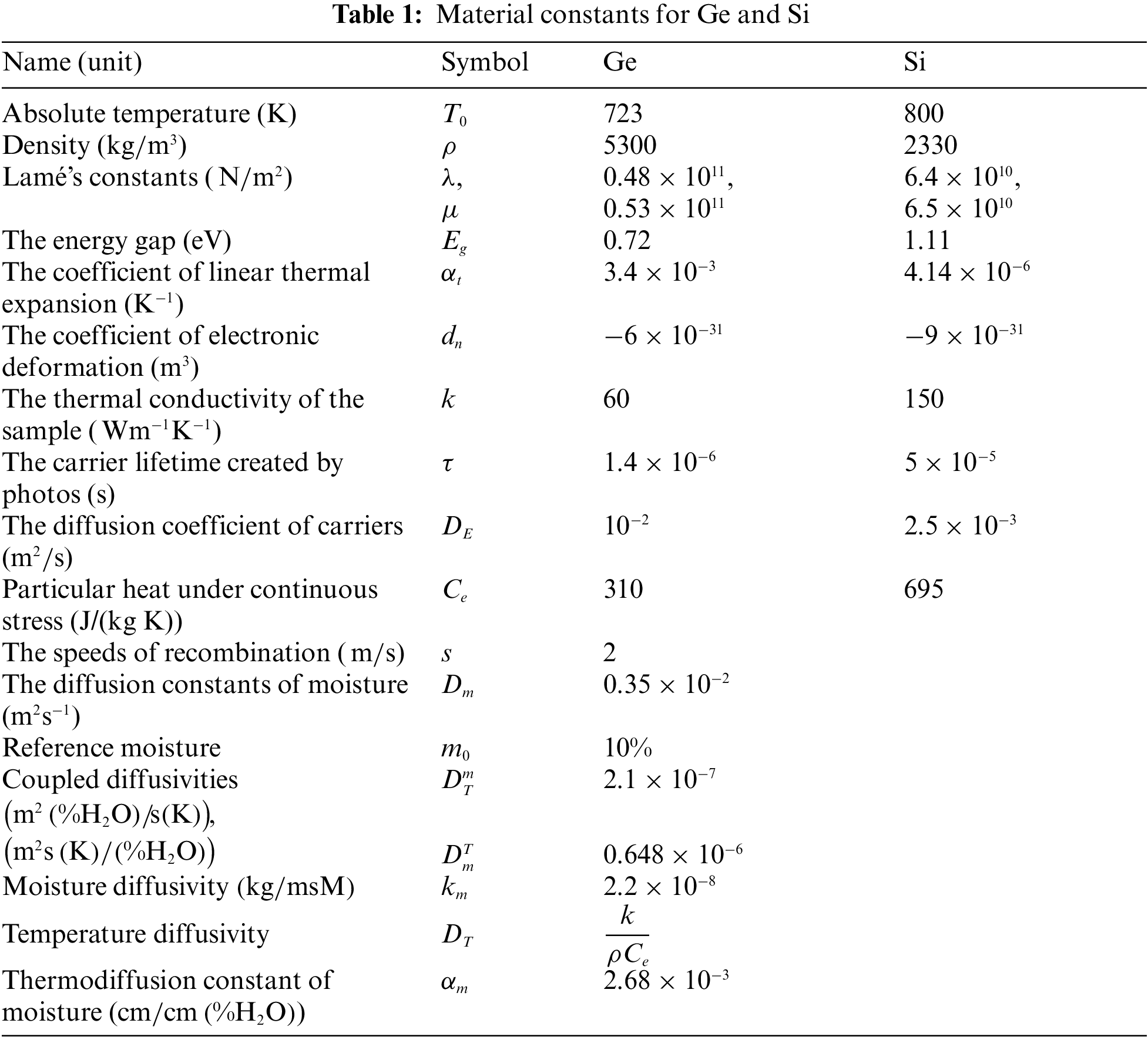
7.1 The Impact of Thermoelastic Coupling Characteristics

According to the principles of photo-thermoelasticity, the representation of physical fields concerning horizontal distance (x) is shown in the first group in Fig. 1. This depiction incorporates the impact of magnetic and rotational fields on moisture diffusivity. The calculations are based on moisture diffusivity for (Si) material, and three examples of the thermoelastic coupling parameter are presented throughout all figures. The red line (____) represents ε1=0.001, the blue line (..........) represents ε1=0.002, and the green line (_ _ _ _) represents ε1=0.003. In the realm of thermoelastic coupling, Fig. 1a illustrates the spatial variation of thermodynamic temperature. To ensure thermal insulation, a minimum positive temperature is necessary. Initially, temperature rises rapidly, eventually plateauing near the surface due to photo-excitation and moisture diffusion. In the subsequent phase, temperature declines to a minimum at a short distance from the surface. Fig. 1b depicts carrier density across varying distances, influenced directly by thermoelastic coupling parameters, maintaining consistency. Fig. 1c illustrates displacement distribution on a rough surface, affected by moisture diffusivity and photothermal excitation, exhibiting an increase towards the surface followed by an exponential decrease. In Fig. 1d, strain distribution due to moisture diffusivity and photo-thermal extinction unfolds, starting positively, peaking negatively, then exponentially declining to zero across different thermoelastic parameter values. Fig. 1e showcases the augmentation of stress force intensity and thermoelastic coupling parameters by mechanical stresses. Lastly, Fig. 1f presents the horizontal distribution of moisture concentration. All three cases have positive moisture concentrations. For the case when ε1=0.001 the distribution takes a smooth reducing exponential behavior. However, when ε1=0.002 and ε1=0.003. The distribution experiences a significant decrease initially, followed by due to the dispersion of moisture, an exponential spread until it approaches a minimum point near to zero [43,44].

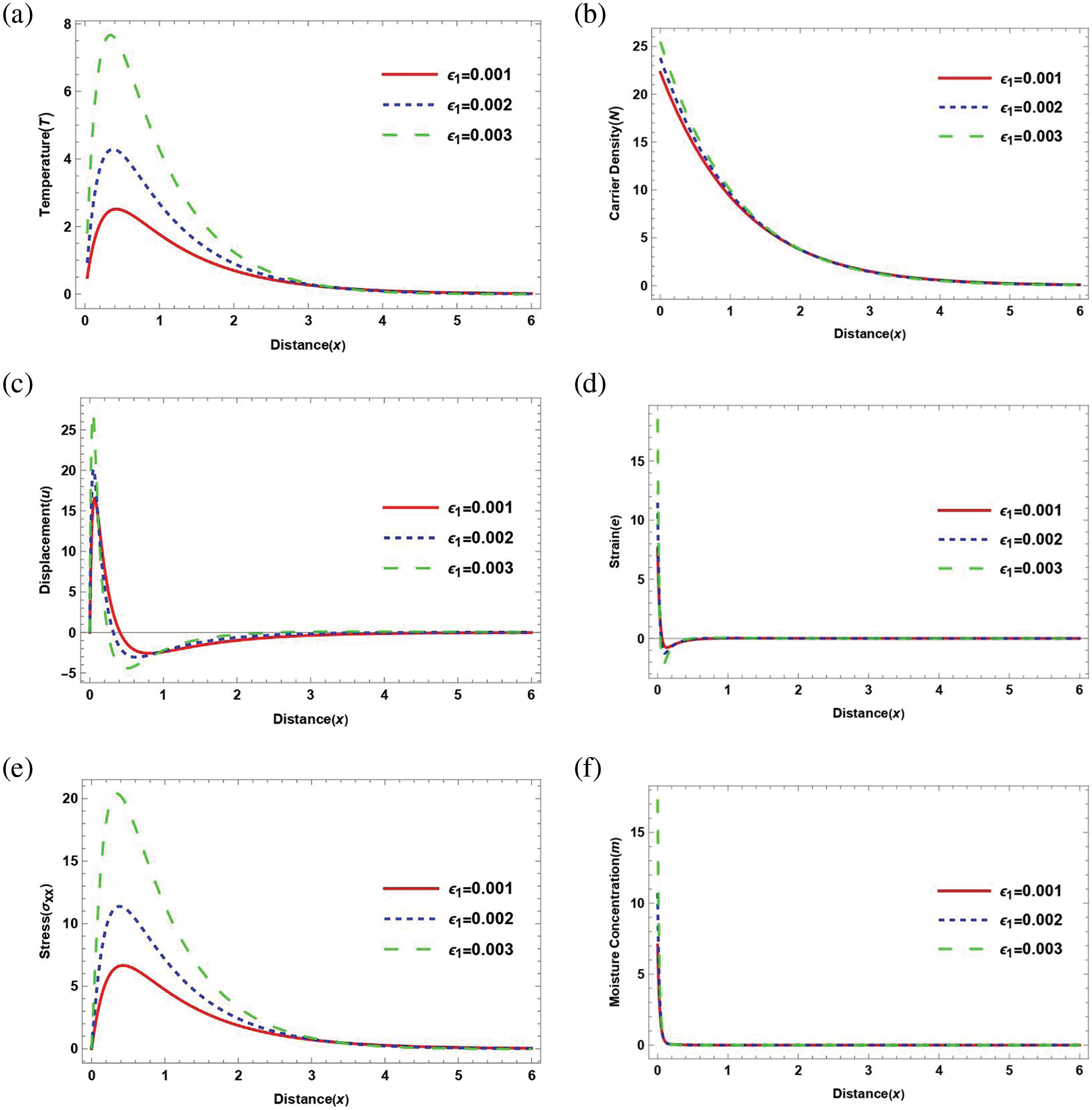
Figure 1: The variation of physical field distributions with distance with the effect of thermoelastic coupling parameter ε1 under the effect of magnetic field H0=105 and Ω=5

7.2 The Effect of the Thermoelectric Coupling Parameter

According to the photo-thermoelasticity theory, Fig. 2 displays the main physical fields in connection to the horizontal distance (x), including moisture diffusivity, magnetic fields, and rotational fields. The moisture diffusivity is taken into account during all calculations. when H0=105 and m0=10% for (Si) material. Three different thermoelectric coupling parameter situations are examined in each of the subfigures. The red line (____) represents ε3=−7.23×10−36 the blue line (.......) expresses ε3=−8.23×10−36 and the green line (_ _ _ _) shows ε3=−9.23×10−36. Altering the dimensionless thermoelectric coupling configurations leads to distinct temperature distributions at varying distances, depicted in Fig. 2a. Initially, temperatures begin at a modest positive level, meeting the criterion for thermal insulation. Subsequently, they swiftly ascend within the first range, peaking near the surface due to photo-excitation and moisture diffusivity. In the succeeding range, temperatures diminish to a minimum well beneath the surface. Fig. 2b illustration demonstrates how carrier density evolves with distance under different thermoelastic parameters. Nevertheless, slight adjustments in thermoelectric coupling parameters have negligible effects on carrier density, which displays consistent behavior. Fig. 2c depiction showcases the horizontal displacement distribution induced by moisture diffusivity and the thermal effects of PT stimulation on a rugged surface. Starting at 0, displacement increases to maximum values close to the surface for all three thermoelectric coupling parameter cases. After then, it drops sharply till it almost reaches zero. The strain distribution with respect to horizontal distance is depicted in Fig. 2d, which is impacted by moisture diffusivity and the thermal consequences of PT stimulation on a rough surface. Commencing from a positive value, strain gradually diminishes to nearly zero levels at the surface across all three scenarios of thermoelectric coupling parameters. The amplitude of the rising stress force brought on by mechanical stresses is depicted in Fig. 2e. Higher thermoelectric coupling parameter values tend to increase this force. Fig. 2f displays the distribution of moisture content for horizontal distance. Within the first range, the concentration drops off dramatically before growing exponentially and eventually reaching a low value close to the zero line. The main factor affecting this behavior is moisture diffusivity.

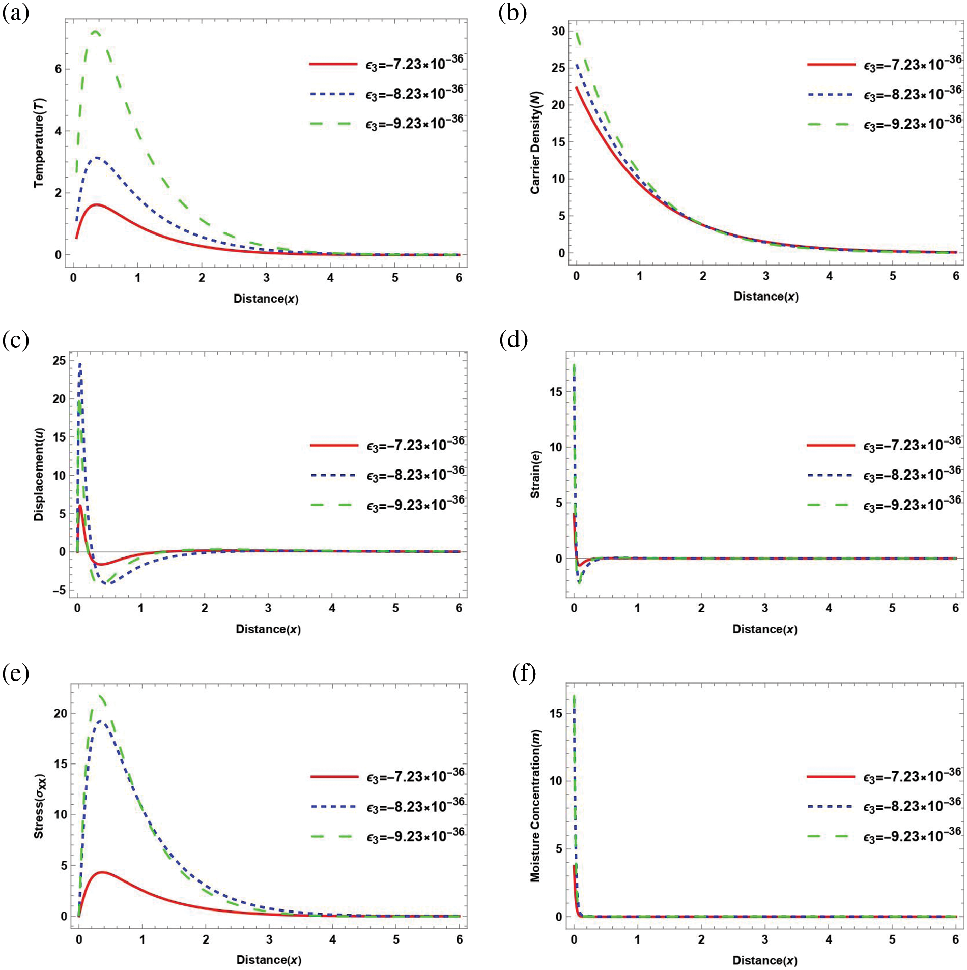
Figure 2: The variation of physical field distributions with distance at different values thermo-electric coupling parameter ε3 under the effect of magnetic field H0=105 and ε1=0.001

7.3 Influence of Rotational Filed

Fig. 3 illustrates the relationship between the horizontal distance and the main physical fields in the third category. It showcases different values of rotational field constants, taking into account the influence of magnetic and moisture diffusivity. All calculations are conducted within the framework of thermally induced mechanical deformations. ε1=0.001, ε3=−7.23×10−36, and magnetic field H0=105 for (Si) material. Fig. 3 illustrates how the physical fields change concerning distance x for three different scenarios of constant rotational field. The first represents the case of rotational felid when Ω=0 (without rotational field) (____), the second case of rotational felid when Ω=0.2 (..........), and the third case of rotational felid when Ω=0.4 (_ _ _ _). This category depicts how the rotational field has a significant impact on the propagation of displacement, strain distribution, stress force, temperature distribution, moisture concentration, and carrier density distribution [45].

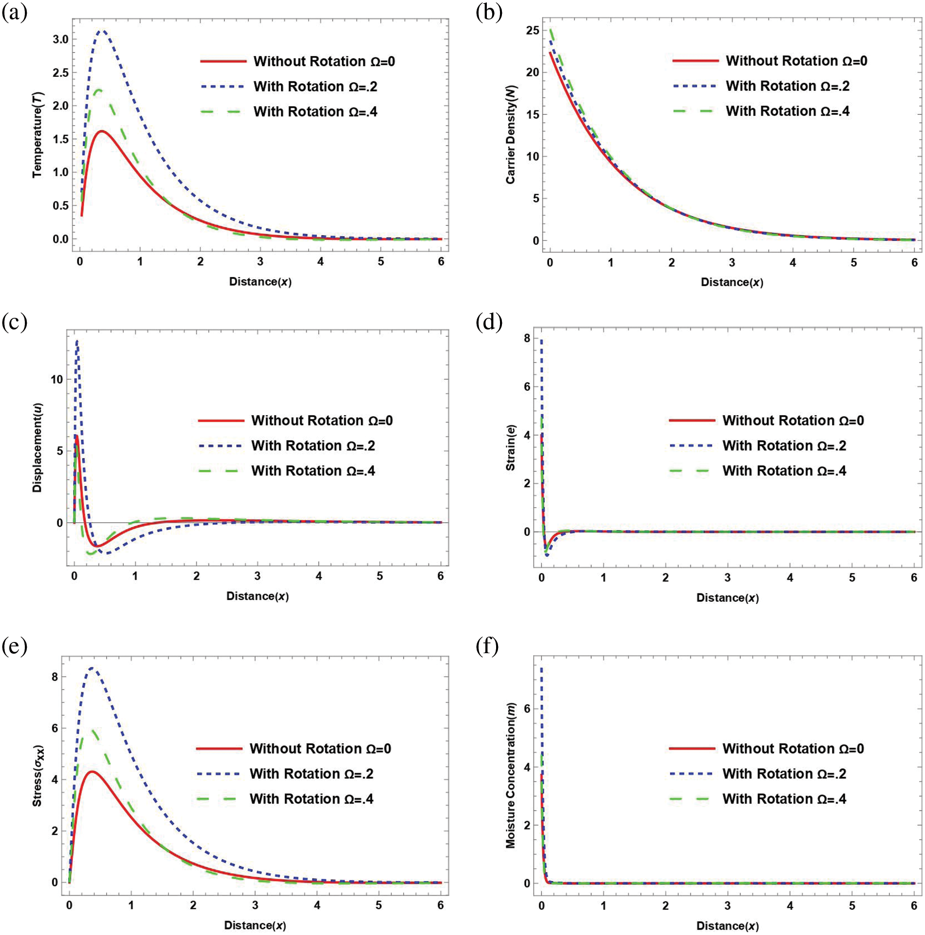
Figure 3: The variation of physical field distributions with distance with the effect of rotational field when ε1=0.001

7.4 Influence of Reference Moisture

Fig. 4 displays the primary physical fields plotted against the horizontal distance. It depicts the variations in moisture constant along with the influence of magnetic and rotational fields in different scenarios. Thermal and elastic coupling are taken into account when conducting all calculations ε1=0.001, ε3=−7.23×10−36 for Silicon (Si) material. Fig. 4 exhibits the variation of the physical fields relative to the distance in three cases of reference moisture m0. The first when m0 = 10% (____), the second when m0 = 20% (.........) and the third when m0 = 30% (_ _ _ _). This category provides evidence that the presence of moisture affects the distributions of temperature, carrier density, stress force, displacement, strain, and moisture concentration as well as how waves propagate.

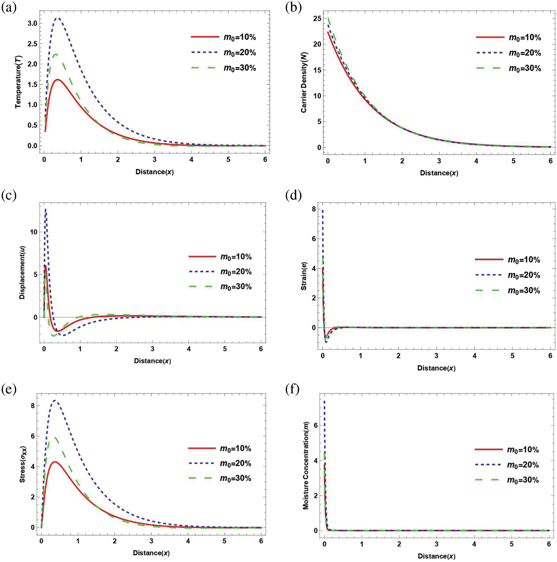
Figure 4: Shows how physical field distributions vary at different distances. The steady state of moisture m0 under the effect of magnetic field H0=105 when ε1=0.001

7.5 Influence of Magnetic Field

The basic physical fields are displayed against a horizontal distance x in Fig. 5, together with various values of the magnetic felid constant and the influence of moisture diffusivity and the rotational field. Every computation is run using thermoelastic couples. ε1=0.001, ε3=−7.23×10−36, and magnetic field Ω=5 for Silicon (Si) material. The fluctuation of the physical fields with respect to distance is shown in three situations of magnetic field constant H0 in Fig. 5. The first represents the case of the magnetic field when H0.0=0 (without magnetic field) (____), the second case of the magnetic field when H0.0=105 (.......), and the third case of the magnetic field when H0.0=5×105 (_ _ _ _). The given information indicates that the magnetic field has an impact on various aspects such as the movement of waves, the concentration of moisture, the force of stress, the distribution of temperature, the distribution of strain, and the density of carriers.

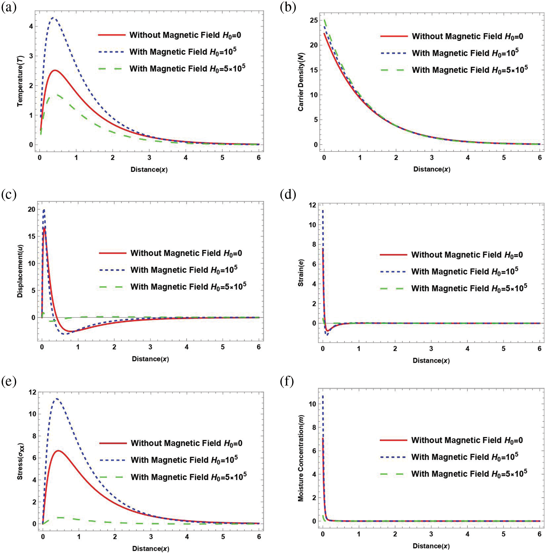
Figure 5: The variation of physical fields distribution under the effect of magnetic field H0 when ε1=0.001 and ε3=−7×10−36

7.6 The Comparison between Ge and Si Materials

Comparison of the elastic semiconductor materials (Si) and (Ge) is shown in Fig. 6. The values of the physical fields under inquiry have been numerically analyzed in this category. when ε1=0.001 and ε3=−7.23×10−36 under the impact of moisture field when m0=10%, magnetic field H0=105, and rotational field Ω=5. The given diagram clearly illustrates that there is a significant contrast in the physical constants of Ge and Si materials, which greatly impact the wave propagation across dimensionless distributions for T, e, u, σ, m and N.

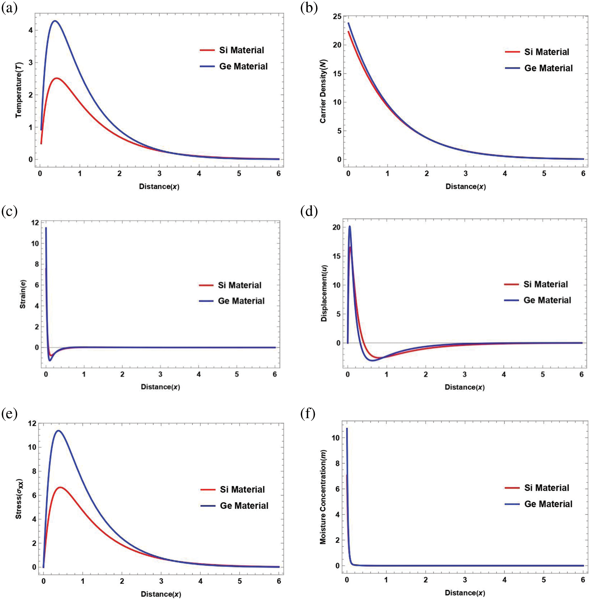
Figure 6: The comparison of physical field distributions with distance under the influence of a magnetic field in Si and Ge materials H0=105 when ε1=0.001

8  Conclusion

This study investigates how various factors influence the transmission of PT-elastic waves in solid semiconductors, particularly focusing on the impact of electron deformation on the material’s deformation potential and wave generation. Using photo-thermoelasticity theory, the research analyzes wave dynamics in semiconductor media, exploring the effects of thermoelasticity, thermoelectricity, magnetic and rotational fields, and moisture concentration on wave propagation. The practical significance of photothermal theory lies in understanding material deexcitation and light absorption. The findings highlight the significant influence of medium properties on the studied aspects, benefiting physicists, material designers, thermal engineers, and geophysicists. The methodology developed offers a tool for addressing various photo-thermoelasticity and thermodynamic challenges. Understanding diffusion phenomena in thermoelasticity has wide implications in engineering, materials science, and biology. Further research in this area promises enhanced comprehension and practical applications. Additionally, studying rotational effects in thermoelasticity is crucial across industries like aerospace, energy, and biomechanics, offering safer solutions to real-world problems.

Acknowledgement: The authors extend their appreciation to Taif University, Saudi Arabia, for supporting this work through Project Number (TU-DSPP-2024-172).

Funding Statement: This research was funded by Taif University, Taif, Saudi Arabia (TU-DSPP-2024-172).

Author Contributions: Khaled Lotfy and A. M. S. Mahdy: Conceptualization, Methodology, Software. E. S. Elidy: Writing—Original draft preparation, Data curation. A. M. S. Mahdy and Alaa A. El-Bary: Supervision, Visualization, Investigation, Software, Validation. All authors: Writing—reviewing and editing. All authors reviewed the results and approved the final version of the manuscript.

Availability of Data and Materials: The data supporting this article are available upon request.

Conflicts of Interest: The study, writing, and publishing of this paper were all done without any possible conflicts of interest disclosed by the authors.

References

1. Szekeres A. Analogy between heat and moisture thermohygro-mechanical tailoring of composites by taking into account the second sound phenomenon. Compute Struct. 2000;76:145–52. [Google Scholar]

2. Szekeres A. Cross-coupled heat and moisture transport: part 1 theory. J Therm Stress. 2012;35:248–68. doi:10.1080/01495739.2012.637827. [Google Scholar] [CrossRef]

3. Gasch T, Malm R, Ansell A. Coupled hygro-thermomechanical model for concrete subjected to variable environmental conditions. Int J Solid Struct. 2016;91:143–56. doi:10.1016/j.ijsolstr.2016.03.004. [Google Scholar] [CrossRef]

4. Povstenko Y. Theories of thermal stresses based on space-time-fractional telegraph equations. Comput Math Appl. 2012;64(10):3321–8. doi:10.1016/j.camwa.2012.01.066. [Google Scholar] [CrossRef]

5. Gordon JP, Leite RCC, Moore RS, Porto SPS, Whinnery JR. Long-transient effects in lasers with inserted liquid samples. Bull Am Phys Soc. 1964;119:501. [Google Scholar]

6. Kreuzer LB. Ultralow gas concentration infrared absorption spectroscopy. J Appl Phys. 1971;42:2934. doi:10.1063/1.1660651. [Google Scholar] [CrossRef]

7. Tam AC. Ultrasensitive laser spectroscopy. New York: Academic Press; 1983. p. 1–108. [Google Scholar]

8. Tam AC. Applications of photoacoustic sensing techniques. Rev Mod Phys. 1986;58:381. doi:10.1103/RevModPhys.58.381. [Google Scholar] [CrossRef]

9. Tam AC. Photothermal investigations in solids and fluids. Boston: Academic Press; 1989. p. 1–33. [Google Scholar]

10. Todorovic DM, Nikolic PM, Bojicic AI. Photoacoustic frequency transmission technique: electronic deformation mechanism in semiconductors. J Appl Phys. 1999;85:7716. doi:10.1063/1.370576. [Google Scholar] [CrossRef]

11. Song YQ, Todorovic DM, Cretin B, Vairac P. Study on the generalized thermoelastic vibration of the optically excited semiconducting microcantilevers. Int J Sol Struct. 2010;47:1871–5. doi:10.1016/j.ijsolstr.2010.03.020. [Google Scholar] [CrossRef]

12. Hobiny A, Abbas IA. A study on photothermal waves in an unbounded semiconductor medium with cylindrical cavity, mech. Time-Depend Mater. 2016;6:1–12. [Google Scholar]

13. Marin M. On existence and uniqueness in thermoelasticity of micropolar bodies. Compt Rendus de l’Acad Sci Paris, Sér II. 1995;321(12):475–80. [Google Scholar]

14. Lotfy KH. Photothermal waves for two temperature with a semiconducting medium under using a dual-phase-lag model and hydrostatic initial stress, Waves Ran. Comp Med. 2017;27(3):482–501. [Google Scholar]

15. Mahdy A, Lotfy KH, El-Bary A, Sarhan H. Effect of rotation and magnetic field on a numerical-refined heat conduction in a semiconductor medium during photo-excitation processes. Eur Phys J Plus. 2021;136:1–17. [Google Scholar]

16. Abo-Dahab S, Lotfy KH, Gohaly A. Rotation and magnetic field effect on surface waves propagation in an elastic layer lying over a generalized thermoelastic diffusive half-space with imperfect boundary. Math Prob Eng. 2015;2015:1–15. [Google Scholar]

17. Lotfy KH, Kumar R, Hassan W, Gabr M. Thermomagnetic effect with microtemperature in a semiconducting Photothermal excitation medium. Appl Math Mech Engl Ed. 2018;39(6):783–96. doi:10.1007/s10483-018-2339-9. [Google Scholar] [CrossRef]

18. Lotfy KH, El-Bary A, El-Sharif A. Ramp-type heating microtemperature for a rotator semiconducting material during photo-excited processes with magnetic field. Results Phys. 2020;19:103338. doi:10.1016/j.rinp.2020.103338. [Google Scholar] [CrossRef]

19. Sur A, Kanoria M. Modeling of fibre-reinforced magneto-thermoelastic plate with heat sources. Proc Eng. 2017;173:875–82. doi:10.1016/j.proeng.2016.12.131. [Google Scholar] [CrossRef]

20. Shakeriaski F, Ghodrat M, Escobedo-Diaz J, Behnia M. Recent advances in generalized thermoelasticity theory and the modified models: a review. J Comput Design Eng. 2021;8(1):15–35. doi:10.1093/jcde/qwaa082. [Google Scholar] [CrossRef]

21. Hasselman D, Heller R. Thermal stresses in severe environments. New York, USA: Plenum Press; 1980. [Google Scholar]

22. Zlatić M, Čanađija M. Incompressible rubber thermoelasticity: a neural network approach. Comput Mech. 2023;71:895–916. doi:10.1007/s00466-023-02278-y. [Google Scholar] [CrossRef]

23. Youssef H, El-Bary A. Thermal shock problem of a generalized thermoelastic layered composite material with variable thermal conductivity. Math Prob Eng. 2006;2006:87940. doi:10.1155/mpe.v2006.1. [Google Scholar] [CrossRef]

24. Youssef H, Abbas I. Thermal shock problem of generalized thermoelasticity for an infinitely long annular cylinder with variable thermal conductivity. Comput Methods Sci Technol. 2007;13(2):95–100. doi:10.12921/cmst. [Google Scholar] [CrossRef]

25. Marin M. An evolutionary equation in thermoelasticity of dipolar bodies. J Math Phys. 1999;40(3):1391–9. doi:10.1063/1.532809. [Google Scholar] [CrossRef]

26. Biot MA. Thermoelasticity and irreversible thermodynamics. J Appl Phys. 1956;27:240–53. doi:10.1063/1.1722351. [Google Scholar] [CrossRef]

27. Lord H, Shulman Y. A generalized dynamical theory of thermoelasticity. J Mech Phys Solids. 1967;15:299–309. doi:10.1016/0022-5096(67)90024-5. [Google Scholar] [CrossRef]

28. Green AE, Lindsay KA. Thermoelasticity. J Elast. 1972;2:1–7. doi:10.1007/BF00045689. [Google Scholar] [CrossRef]

29. Chandrasekharaiah DS. Thermoelasticity with second sound: a review. Appl Mech Rev. 1986;39:355–76. doi:10.1115/1.3143705. [Google Scholar] [CrossRef]

30. Hosseini SM, Sladek J, Sladek V. Application of meshless local integral equations to two dimensional analysis of coupled non-Fick diffusion-elasticity. Eng Anal Boundary Elem. 2014;37(3):603–15. [Google Scholar]

31. Lata P, Kaur H. Deformation in a homogeneous isotropic thermoelastic solid with multi-dual-phase-lag heat & two temperature using modified couple stress theory. Compos Mater Eng. 2021;3(2):89–106. [Google Scholar]

32. Lata P. Fractional effect in an orthotropic magneto-thermoelastic rotating solid of type GN-II due to normal force. Struct Eng Mech. 2022;81(4):503–11. [Google Scholar]

33. Marin M, Öchsner A, Bhatti M. Some results in Moore-Gibson-Thompson thermoelasticity of dipolar bodies, (ZAMM) Zfur Angew. Math Mech. 2020;100(12):e202000090. [Google Scholar]

34. Roy S, Lahiri A. Fractional order thermoelastic model with voids in three-phase-lag thermoelasticity. Comput Sci Math Forum. 2023;7:57. [Google Scholar]

35. Lotfy KH, El-Bary A, Tantawi RS. Effects of variable thermal conductivity of a small semiconductor cavity through the fractional order heat-magneto-photothermal theory. Eur Phys J Plus. 2019;134(6):280. doi:10.1140/epjp/i2019-12631-1. [Google Scholar] [CrossRef]

36. Lotfy KH, Elidy E, Tantawi R. Photothermal excitation process during hyperbolic two-temperature theory for magneto-thermo-elastic semiconducting medium. Silicon. 2021;13:2275–88. doi:10.1007/s12633-020-00795-6. [Google Scholar] [CrossRef]

37. Ailawalia P, Priyanka. Effect of thermal conductivity in a semiconducting medium under modified Green-Lindsay theory. Int J Comput Sci Math. 2024;19(2):167–79. doi:10.1504/IJCSM.2024.137263. [Google Scholar] [CrossRef]

38. Honig G, Hirdes U. A method for the numerical inversion of Laplace Transforms. J Comput Appl Math. 1984;10(1):113–32. doi:10.1016/0377-0427(84)90075-X. [Google Scholar] [CrossRef]

39. Lotfy KH, Elidy E, Tantawi R. Piezo-photo-thermoelasticity transport process for hyperbolic two-temperature theory of semiconductor material. Int J Mod Phys C. 2021;32(7):2150088. doi:10.1142/S0129183121500881. [Google Scholar] [CrossRef]

40. Marin M. Harmonic vibrations in thermoelasticity of microstretch materials. J Vib Acoust Trans ASME. 2010;132(4):44501. doi:10.1115/1.4000971. [Google Scholar] [CrossRef]

41. Mondal S, Sur A. Photo-thermo-elastic wave propagation in an orthotropic se miconductor with a spherical cavity and memory responses. Waves Random Complex Med. 2021;31(6):1835–58. doi:10.1080/17455030.2019.1705426. [Google Scholar] [CrossRef]

42. Bazarra N, Fernández JR, Liverani L, Quintanilla R. Analysis of a thermoelastic problem with the Moore-Gibson–Thompson microtemperatures. J Comput Appl Math. 2024;438:115571. doi:10.1016/j.cam.2023.115571. [Google Scholar] [CrossRef]

43. Ezzat M. A novel model of fractional thermal and plasma transfer within a non-metallic plate. Smart Stru Syst. 2021;27(1):73–87. [Google Scholar]

44. Kaur I, Kulvinder S, Eduard-Marius C. A mathematical study of a semiconducting thermoelastic rotating solid cylinder with modified Moore-Gibson–Thompson heat transfer under the hall effect. Mathematics. 2022;10(14):2386. doi:10.3390/math10142386. [Google Scholar] [CrossRef]

45. Abouelregal A. Magneto-photothermal interaction in a rotating solid cylinder of semiconductor silicone material with time dependent heat flow. Appl Math Mech. 2021;42(1):39–52. doi:10.1007/s10483-021-2682-6. [Google Scholar] [CrossRef]